

Learn VaR calculation using parametric, historical, and Monte Carlo methods. Explore Expected Shortfall and stress testing for market risk management.
Choose your expertise level to adjust how many terms are explained. Beginners see more tooltips, experts see fewer to maintain reading flow. Hover over underlined terms for instant definitions.
Market Risk Measurement - VaR and Beyond
The collapse of Barings Bank in 1995 and the near-failure of Long-Term Capital Management in 1998 demonstrated that even sophisticated financial institutions could face catastrophic losses from market risk exposures they poorly understood. These events accelerated the adoption of Value-at-Risk (VaR), a deceptively simple metric that answers a question every risk manager needs answered: "How bad could things get?"
VaR distills the complexity of a portfolio's risk exposures into a single number representing the maximum expected loss over a specified time horizon at a given confidence level. If a portfolio has a one-day 99% VaR of $10 million, this means that under normal market conditions, the portfolio should not lose more than $10 million in a single day with 99% probability. Equivalently, losses exceeding $10 million should occur only about 1% of trading days, or roughly 2-3 times per year.
The Basel Committee on Banking Supervision embedded VaR into the regulatory framework for bank capital requirements in 1996, cementing its role as the industry standard for market risk measurement. However, the 2008 financial crisis exposed serious limitations: VaR tells you where the cliff is but not how far you might fall. This chapter develops VaR from first principles, implements the three major calculation methods, and then moves beyond VaR to Expected Shortfall and stress testing techniques that address its shortcomings.
The VaR Framework
Before diving into calculation methods, we need to establish the formal definition of VaR and understand what it does and does not measure. At its heart, VaR addresses a fundamental question in risk management: given the inherent uncertainty in financial markets, what is the worst loss we should reasonably expect under normal conditions? The answer requires us to think probabilistically about potential outcomes rather than seeking a single deterministic prediction.
We cannot know exactly what loss will occur tomorrow. Instead, we can characterize the full distribution of possible losses and then identify a threshold that separates "normal" adverse outcomes from truly extreme events. This threshold becomes our VaR estimate. By specifying a confidence level, we acknowledge that losses beyond this threshold will sometimes occur, but we want such exceedances to be rare enough that we consider them exceptional rather than routine.
The Value-at-Risk at confidence level over time horizon is defined as the smallest loss such that the probability of experiencing a loss greater than is at most :
where:
- : Value-at-Risk at confidence level
- : a potential loss value
- : portfolio loss (positive values indicate losses)
- : confidence level
- : infimum (smallest value)
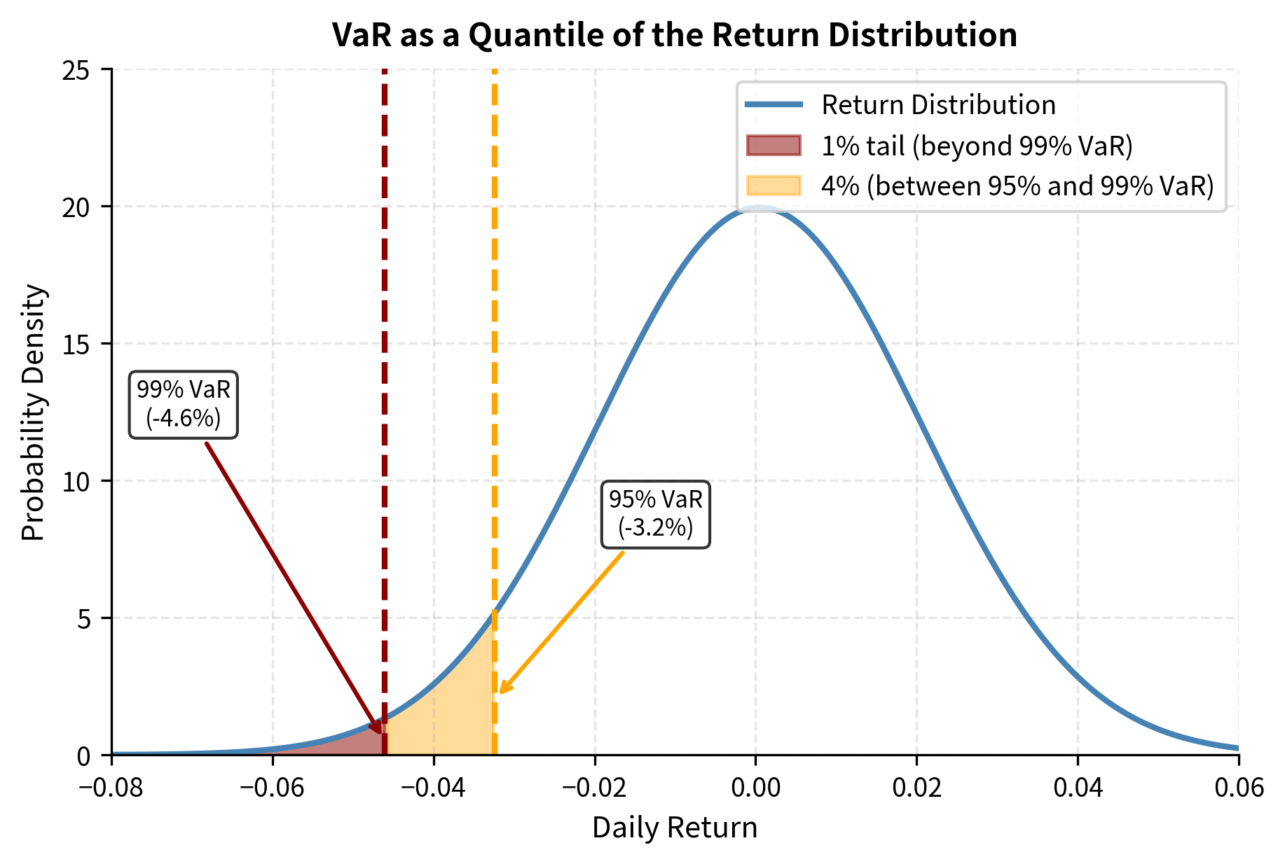
Equivalently, VaR is the -quantile of the loss distribution.
This formal definition uses the infimum (greatest lower bound) to handle distributions that may have discontinuities or discrete probability masses. For most practical purposes with continuous return distributions, you can think of VaR simply as the loss value that separates the worst fraction of outcomes from the better fraction. The definition ensures that we identify the precise point on the loss distribution where cumulative probability reaches our target confidence level.
VaR depends on three key parameters:
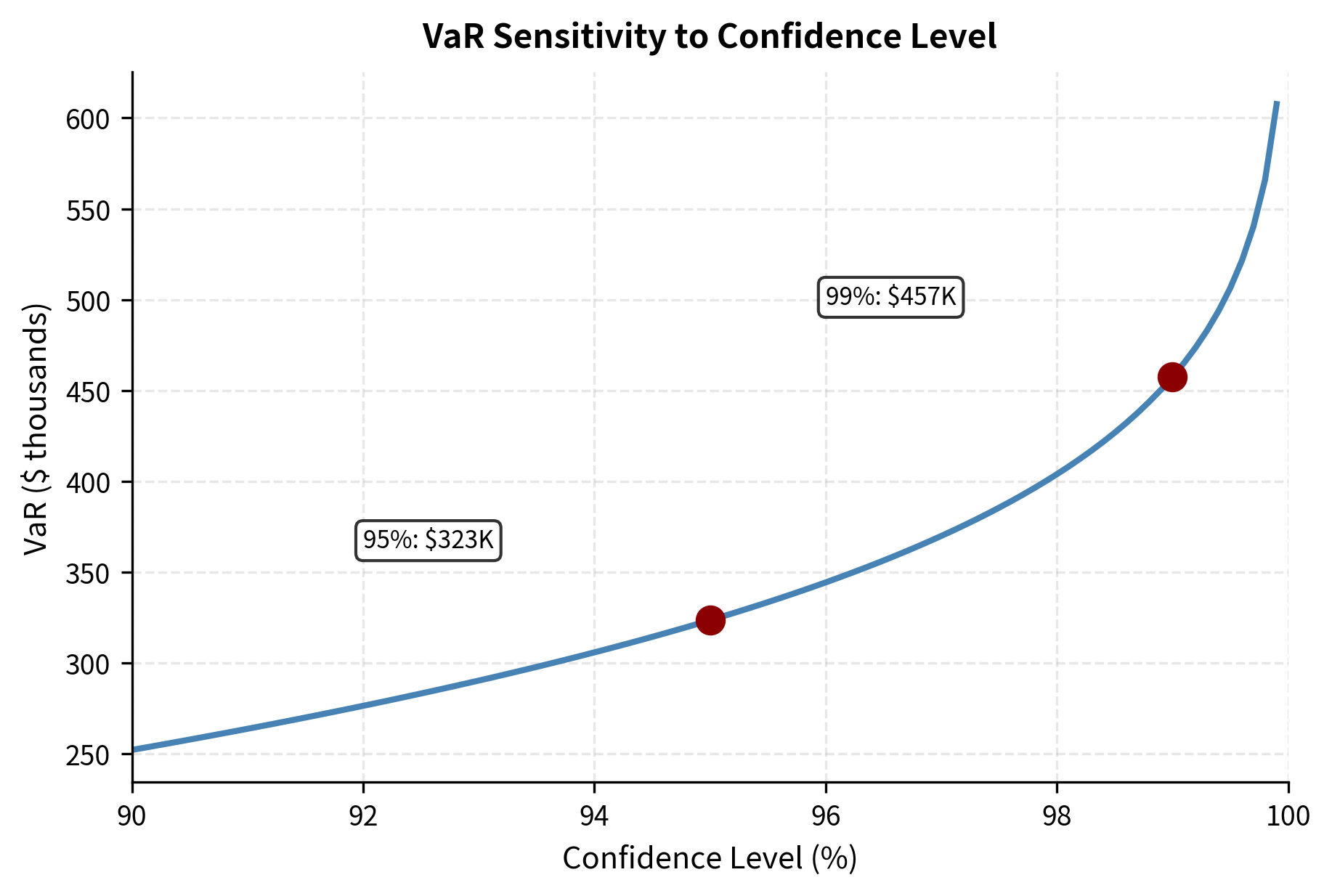
- Confidence level (): Typically 95% or 99%. Higher confidence levels produce larger VaR estimates but are harder to backtest due to fewer tail observations.
- Time horizon (): Usually 1 day for trading desks or 10 days for regulatory capital calculations. Longer horizons capture more risk but assume portfolio composition remains static.
- Portfolio value: VaR is typically expressed in absolute currency terms, though it can also be expressed as a percentage of portfolio value.
The sign convention varies in practice. Some practitioners define VaR as a positive number representing potential loss, while others express it as a negative return. We follow the convention where VaR is positive, so a VaR of $10 million means the portfolio could lose up to $10 million.
Relationship to Return Distributions
Understanding how VaR connects to the underlying return distribution is essential for all calculation methods. This relationship provides the mathematical bridge between the abstract definition of VaR and the practical task of computing it from return data or models.
For a portfolio with current value and return over the horizon, the loss is (since negative returns create positive losses). This transformation is crucial: when we observe a return of -3%, the portfolio experiences a positive loss equal to 3% of its value. By expressing everything in terms of losses, we ensure that VaR comes out as a positive number that can be directly interpreted as potential monetary damage.
If returns follow a continuous distribution with cumulative distribution function , then VaR at confidence level corresponds to the quantile of the return distribution:
where:
- : Value-at-Risk at confidence level
- : current portfolio value
- : inverse cumulative distribution function of returns
- : probability level for the tail
To understand why VaR uses the quantile rather than the quantile, consider what we are seeking. For 99% VaR, we want the loss that is exceeded only 1% of the time. This corresponds to returns that fall below the 1st percentile of the return distribution. The inverse CDF gives us exactly this value: the return below which only 1% of outcomes fall. Multiplying by converts this worst-case return into the corresponding dollar loss.
This relationship is the foundation for all VaR calculation methods. The methods differ in how they estimate the return distribution and its quantiles. Parametric methods assume a specific distributional form and estimate its parameters. Historical simulation uses the empirical distribution directly. Monte Carlo simulation generates a synthetic distribution from a specified stochastic model. Each approach represents a different answer to the question: "How do we characterize the distribution of portfolio returns?"
Parametric VaR: The Variance-Covariance Method
The parametric approach assumes portfolio returns follow a known distribution, typically the normal distribution. This allows closed-form calculation of VaR using only the mean and standard deviation of returns.
The parametric method is simple and computationally efficient. If we accept the assumption that returns are normally distributed, we can exploit the well-known properties of the normal distribution to derive an explicit formula for VaR. This avoids the need for simulation or extensive historical databases, making the method particularly attractive for large portfolios where computational speed matters.
Single-Asset Parametric VaR
For a single asset with normally distributed returns having mean and standard deviation , we can determine any quantile of the distribution using the standard normal transformation. The key insight is that any normal distribution can be expressed as a linear transformation of the standard normal distribution, which has mean zero and standard deviation one.
The quantile of returns is:
where:
- : quantile of returns
- : mean return
- : return standard deviation
- : quantile of the standard normal distribution
This formula follows directly from the properties of normal distributions. If , then follows the standard normal . Solving for at the point where gives us the quantile formula above.
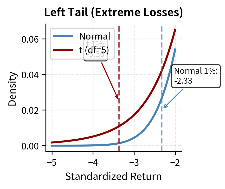
For common confidence levels, and . These values indicate how many standard deviations below the mean we must go to reach the specified tail probability. The negative sign reflects that we are looking at the left tail of the distribution, where the worst returns reside.
The parametric VaR for a portfolio of value is derived by scaling the return quantile by the portfolio value:
where:
- : Value-at-Risk
- : portfolio value
- : expected return
- : volatility
- : standard normal quantile
Let us trace through this derivation more carefully. We start with the relationship , which converts the worst expected return into a dollar loss. Substituting our expression for the return quantile, we obtain . Since is negative for tail quantiles (we are looking at returns below the mean), the product is also negative, and subtracting this negative quantity effectively adds a positive risk term.
For short time horizons like one day, the expected return is typically negligible compared to volatility (). To see why, consider that a typical stock might have an expected daily return of 0.04% (about 10% annualized), while daily volatility might be 2%. The volatility term dominates the calculation by roughly a factor of 50. Since is negative for tail quantiles, , allowing us to simplify:
where:
- : simplified Value-at-Risk
- : portfolio value
- : volatility
- : absolute value of the quantile (e.g., 1.645 for 95% confidence)
This simplified formula reveals the intuitive structure of parametric VaR. The risk measure is proportional to portfolio value, volatility, and a multiplier that depends on the confidence level. For 95% confidence, the multiplier is 1.645; for 99% confidence, it increases to 2.326. This scaling reflects the deeper penetration into the tail required for higher confidence levels.
Let's implement this for a stock portfolio using historical data to estimate volatility:
The 99% VaR of approximately $460,000 means we expect daily losses to exceed this amount only about 1% of trading days, roughly 2-3 times per year.
Multi-Asset Parametric VaR
For a portfolio of multiple assets, we need to account for correlations between asset returns. As we discussed in Part IV on Modern Portfolio Theory, the variance of a portfolio depends on the covariance matrix of its constituents. When assets move together, portfolio risk is higher; when they move independently or inversely, diversification reduces total risk below the weighted sum of individual risks.
The mathematical framework for multi-asset VaR builds directly on portfolio theory. Consider a portfolio with assets, where we invest fraction in asset . The portfolio return is the weighted sum of individual returns: . Since the sum of normally distributed random variables is also normal, the portfolio return inherits normality from its constituents.
For a portfolio with weight vector and asset covariance matrix , the portfolio variance is:
where:
- : portfolio variance
- : vector of portfolio weights
- : covariance matrix of asset returns
- : transpose operator
This quadratic form captures all pairwise interactions between assets. The diagonal elements of contribute weighted variances, while the off-diagonal elements contribute weighted covariances. When assets are less than perfectly correlated, the cross-product terms partially cancel, reducing portfolio variance below what a simple weighted average would suggest.
The parametric VaR extends naturally by substituting portfolio volatility into our single-asset formula:
where:
- : Value-at-Risk
- : total portfolio value
- : weight vector
- : covariance matrix
- : standard normal quantile
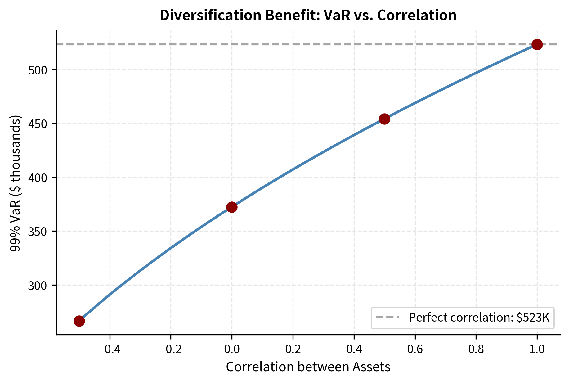
This formula demonstrates that portfolio VaR depends on the entire covariance structure, not just individual asset volatilities. Two portfolios with identical asset volatilities can have dramatically different VaR depending on their correlation structure. A portfolio of highly correlated assets concentrates risk, while a portfolio of uncorrelated or negatively correlated assets disperses it.
Notice that the portfolio volatility (approximately 1.7%) is lower than a simple weighted average of individual volatilities would suggest. This is the diversification benefit: imperfect correlations reduce portfolio risk.
Advantages and Limitations of Parametric VaR
The parametric method has compelling advantages. It is computationally fast, requires only estimates of means, volatilities, and correlations, and provides intuitive decomposition of risk contributions. Financial institutions with thousands of positions can compute VaR almost instantaneously.
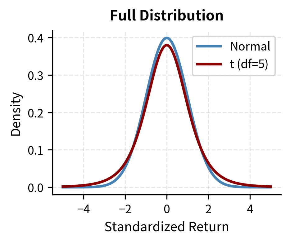
However, the normality assumption is problematic. As we explored in the chapter on Stylized Facts of Financial Returns, actual return distributions exhibit fat tails and excess kurtosis. The normal distribution underestimates the probability of extreme events. A return of 4 standard deviations should occur about once every 126 years under normality, yet markets regularly experience such moves several times per decade.
Historical Simulation VaR
Historical simulation sidesteps distributional assumptions by using the actual empirical distribution of past returns. The method revalues the portfolio using historical return scenarios and directly reads VaR from the resulting distribution of portfolio values.
Historical simulation avoids theoretical models by using actual data. Whatever patterns exist in historical returns, including fat tails, skewness, and complex dependencies, are automatically captured when we use actual historical scenarios as the basis for risk measurement.
The Historical Simulation Approach
The procedure begins by assembling a database of historical returns for all assets in the portfolio. Each historical day provides one complete scenario: a vector of returns for every asset that actually occurred together in the market. This preserves the natural co-movement patterns that existed on each date, including any unusual correlation structures during market stress periods.
The steps proceed systematically:
- Collect historical returns for all portfolio assets over a lookback window (typically 250-500 days)
- Apply each historical return scenario to the current portfolio
- Calculate the portfolio profit or loss for each scenario
- Sort the P&L outcomes and select the appropriate quantile as VaR
For 500 historical observations and 99% confidence, VaR is the 5th worst loss (since 1% of 500 is 5).
The key conceptual shift from parametric VaR is that we no longer assume any particular distributional form. Instead, we treat the historical return vectors as equally likely future scenarios. Each past day contributes one potential outcome, and the empirical distribution of these outcomes becomes our estimate of the true return distribution. VaR is then read directly from this empirical distribution as the appropriate order statistic.
The historical simulation results are subject to sampling noise given the limited history (504 days). With 99% confidence, we are looking at the 5th or 6th worst outcome, making the estimate sensitive to individual extreme points in the dataset.
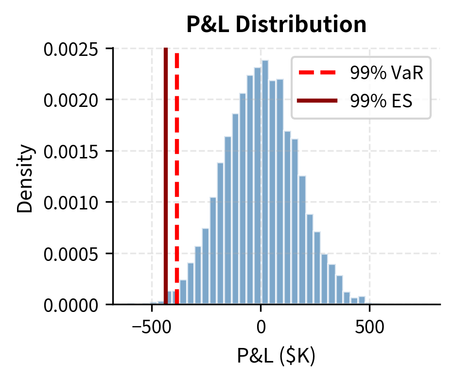
Visualizing the P&L Distribution
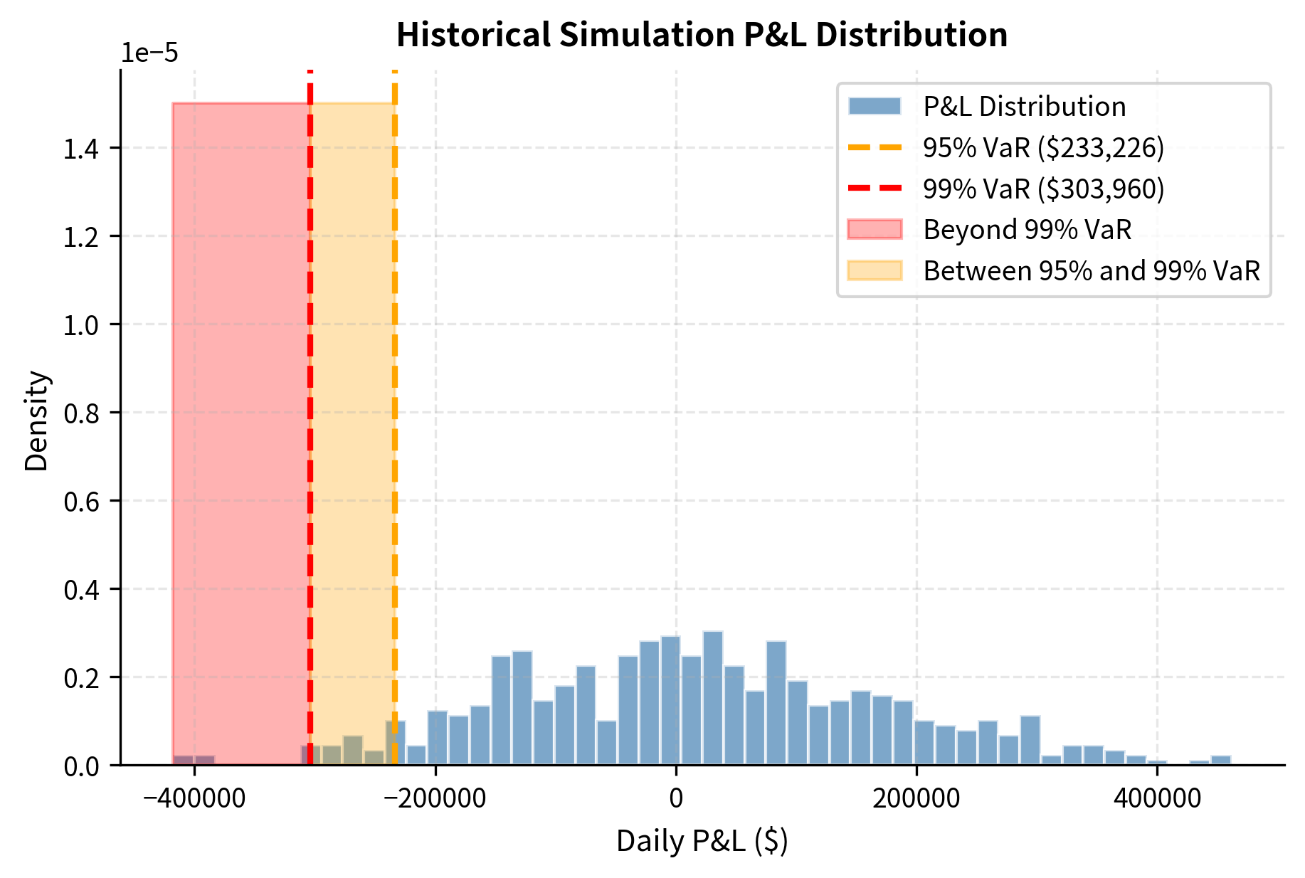
The histogram shows that losses beyond the 99% VaR threshold are rare but do occur. Historical simulation captures the actual shape of the return distribution, including any fat tails present in the data.
Advantages and Limitations of Historical Simulation
Historical simulation requires no distributional assumptions and automatically captures fat tails, skewness, and nonlinear dependencies present in historical data. It handles options and other nonlinear instruments naturally since you revalue the actual portfolio under each scenario.
The method has significant drawbacks, however. It assumes the past is representative of the future: if the lookback window contains only calm markets, VaR will underestimate risk. The method is also sensitive to the choice of window length. Too short a window produces noisy estimates; too long a window includes stale data that may no longer reflect current market dynamics. Additionally, rare extreme events in the lookback period can cause VaR to jump discontinuously as those observations enter or exit the window.
Monte Carlo VaR
Monte Carlo simulation combines the flexibility of historical simulation with the ability to model forward-looking dynamics. Rather than using actual historical returns, Monte Carlo VaR generates scenarios from a specified stochastic model of asset returns.
Monte Carlo simulation overcomes the lack of extreme events in historical data. By specifying a stochastic model, we can generate arbitrarily many scenarios, including rare combinations that have never occurred historically but remain plausible. This allows us to explore the full range of potential outcomes implied by our risk model.
The Monte Carlo Approach
Building on our coverage of Monte Carlo simulation in Part III for derivative pricing, the procedure for VaR is analogous:
- Specify a stochastic model for asset returns (e.g., multivariate normal, multivariate t, or more complex dynamics)
- Estimate model parameters from historical data
- Generate thousands of random scenarios from the model
- Revalue the portfolio under each scenario
- Calculate VaR from the simulated P&L distribution
The key advantage is flexibility: you can incorporate time-varying volatility (such as GARCH models we studied in Part III), fat-tailed distributions, or scenario-specific assumptions.
The quality of Monte Carlo VaR depends critically on the specified model. If the model accurately captures the true dynamics of asset returns, the simulated distribution will converge to the true distribution as the number of scenarios increases. However, if the model is misspecified, even infinitely many simulations will converge to the wrong answer. This emphasizes that Monte Carlo simulation does not eliminate model risk; it merely shifts the burden from distributional assumptions to model specification.
These results are similar to the parametric method because the underlying simulation used a normal distribution and the same covariance structure. The slight differences arise from sampling noise in the random number generation, which would decrease as the number of simulations increases.
Monte Carlo VaR with Fat Tails
To address the fat-tail problem, we can replace the normal distribution with a Student's t-distribution, which has heavier tails controlled by the degrees of freedom parameter . Lower values of produce fatter tails; as , the t-distribution converges to the normal.
The t-distribution provides a natural extension that preserves much of the mathematical tractability of the normal while allowing for heavier tails. Empirical studies suggest that financial returns are often well-approximated by t-distributions with degrees of freedom between 3 and 8, depending on the asset class and time period. The choice of represents a modeling decision about how fat we believe the tails to be.
Constructing multivariate t-distributed random variables requires a subtle technique. We cannot simply substitute t-distributed marginals into a correlation structure because that would not produce the correct joint distribution. Instead, we exploit a mathematical property: a multivariate t-distribution can be represented as a multivariate normal divided by an independent chi-squared random variable. This representation allows us to generate correlated t-distributed returns while preserving the desired dependency structure.
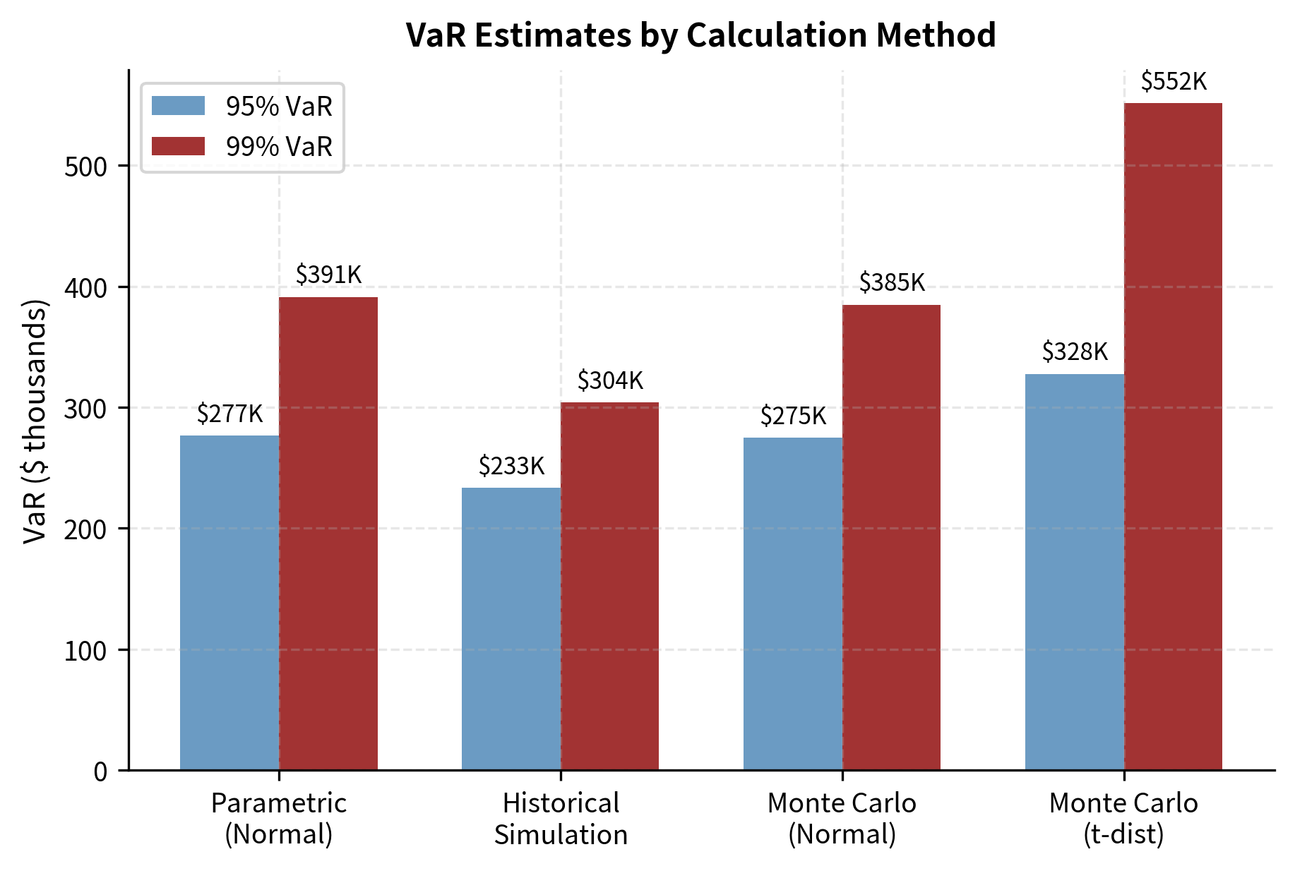
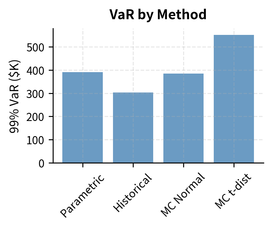
The t-distribution produces substantially higher VaR estimates, particularly at the 99% level where tail behavior dominates. This illustrates why distributional assumptions matter significantly for risk measurement.
Comparing All Three Methods
Limitations of VaR
Despite its widespread adoption, VaR has fundamental limitations that became painfully apparent during the 2008 financial crisis. Understanding these limitations is essential for proper risk management.
VaR Tells You Nothing About Tail Severity
The most critical limitation is that VaR is silent about losses beyond the threshold. A 99% VaR of $10 million says losses will exceed this level 1% of the time, but it provides no information about whether those tail losses average $11 million or $50 million. Two portfolios with identical VaR can have vastly different risk profiles in the tail.
Consider a portfolio that sells deep out-of-the-money options. Most days it earns small premium income, producing a favorable VaR. But on the rare days when the options go in-the-money, losses can be catastrophic. VaR completely misses this asymmetric risk profile.
VaR Is Not Sub-Additive
A mathematically troubling property is that VaR can violate sub-additivity: the VaR of a combined portfolio can exceed the sum of individual VaRs. This means diversification can appear to increase risk under VaR, which contradicts financial intuition and makes risk aggregation problematic.
A risk measure is coherent if it satisfies four axioms:
- Monotonicity: If portfolio A always loses more than portfolio B, then
- Sub-additivity: (diversification reduces risk)
- Positive homogeneity: for (doubling position doubles risk)
- Translation invariance: Adding cash reduces risk by the cash amount
VaR satisfies all axioms except sub-additivity for general distributions.
Backtesting Challenges
Validating VaR models requires backtesting: comparing predicted VaR to actual realized P&L. For 99% VaR, you expect exceedances about 1% of trading days. With 250 trading days per year, that's only 2-3 expected exceedances, making it statistically difficult to distinguish a good model from a bad one. You need years of data to have statistical power, but by then market dynamics may have changed.
Model Risk and Parameter Uncertainty
All three VaR methods depend on historical data to estimate parameters or scenarios. When markets enter regimes not represented in the lookback period, VaR estimates can be dangerously wrong. The 2008 crisis saw correlations spike toward 1.0 across asset classes, volatilities explode, and return distributions shift dramatically. VaR models calibrated to pre-crisis data severely underestimated risk.
Expected Shortfall: A Coherent Alternative
Expected Shortfall (ES), also known as Conditional VaR (CVaR) or Average VaR, addresses VaR's silence about tail severity by measuring the average loss given that the loss exceeds VaR.
Expected Shortfall accounts for the entire tail rather than just the threshold. VaR marks the boundary of the danger zone, but Expected Shortfall tells us the average severity of outcomes within that zone. This provides a more complete picture of tail risk exposure.
Expected Shortfall at confidence level is the expected loss conditional on the loss exceeding VaR:
where:
- : Expected Shortfall at confidence level
- : expected value operator
- : portfolio loss
- : Value-at-Risk threshold
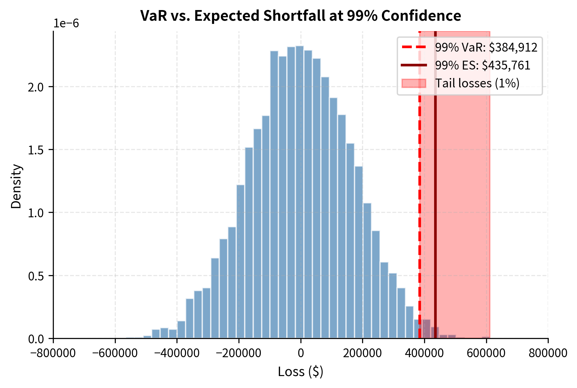
Equivalently, ES is the average of all losses in the tail beyond VaR.
The definition has a clear practical interpretation. Expected Shortfall answers the question: "Given that we have entered the danger zone, how bad do things typically get?" This conditional expectation provides exactly the information that VaR withholds.
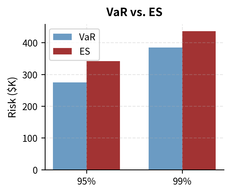
Expected Shortfall is always greater than or equal to VaR at the same confidence level, and it satisfies sub-additivity, making it a coherent risk measure. The Basel Committee recognized these advantages and incorporated ES into the Basel III framework, requiring banks to calculate 97.5% ES for market risk capital.
Calculating Expected Shortfall
For historical simulation or Monte Carlo, ES is simply the average of losses beyond the VaR threshold. This calculation is straightforward once we have generated or collected the distribution of portfolio outcomes:
Expected Shortfall is consistently higher than VaR because it averages all losses in the tail rather than just identifying the threshold. The difference is most pronounced in the t-distribution model, where fat tails lead to significantly larger expected losses beyond the VaR cutoff.
Parametric Expected Shortfall
For normally distributed returns, Expected Shortfall has a closed-form solution that follows from the properties of the truncated normal distribution. The derivation involves computing the expected value of a normal random variable conditional on it falling below a specified threshold.
where:
- : Expected Shortfall
- : portfolio value
- : volatility
- : standard normal probability density function
- : quantile of standard normal distribution
- : tail probability
The term (often called the inverse Mills ratio) represents the expected value of the standardized tail. It tells us how far the average tail event is from the mean in standard deviation units. To understand this intuitively, consider that the density function measures how much probability mass exists exactly at the VaR threshold, while the denominator is the total probability in the tail. Their ratio captures the shape of the tail and determines how far beyond VaR we expect to go on average.
By multiplying this factor by the portfolio volatility and value , we convert the standardized tail expectation into a currency loss. This formula connects the properties of the normal distribution to practical risk measurement.
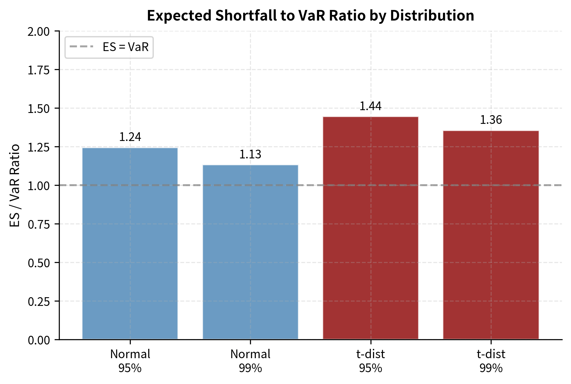
For the normal distribution, the ratio of ES to VaR is relatively stable (approximately 1.15 for 99% confidence). This ratio is often used as a rule of thumb, but it dangerously underestimates tail risk if the underlying distribution has fat tails (excess kurtosis).
Visualizing VaR vs. Expected Shortfall
Stress Testing and Scenario Analysis
VaR and ES are statistical measures based on historical patterns or distributional assumptions. Stress testing complements these by explicitly examining portfolio performance under extreme but plausible scenarios that may not be well-represented in historical data.
Historical Stress Tests
Historical stress tests revalue the portfolio using returns from actual crisis periods. This ensures the scenarios are internally consistent: correlations, volatility spikes, and return magnitudes all reflect what actually happened in real market dislocations.
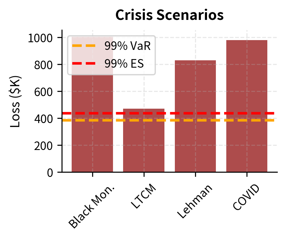
Common historical stress scenarios include:
- Black Monday (October 19, 1987): S&P 500 fell 22.6% in a single day
- LTCM Crisis (August 1998): Flight to quality crushed credit spreads while equity volatility spiked
- Global Financial Crisis (September-October 2008): Broad market declines with correlation breakdown
- COVID Crash (March 2020): Rapid 34% decline in equities with liquidity dislocations
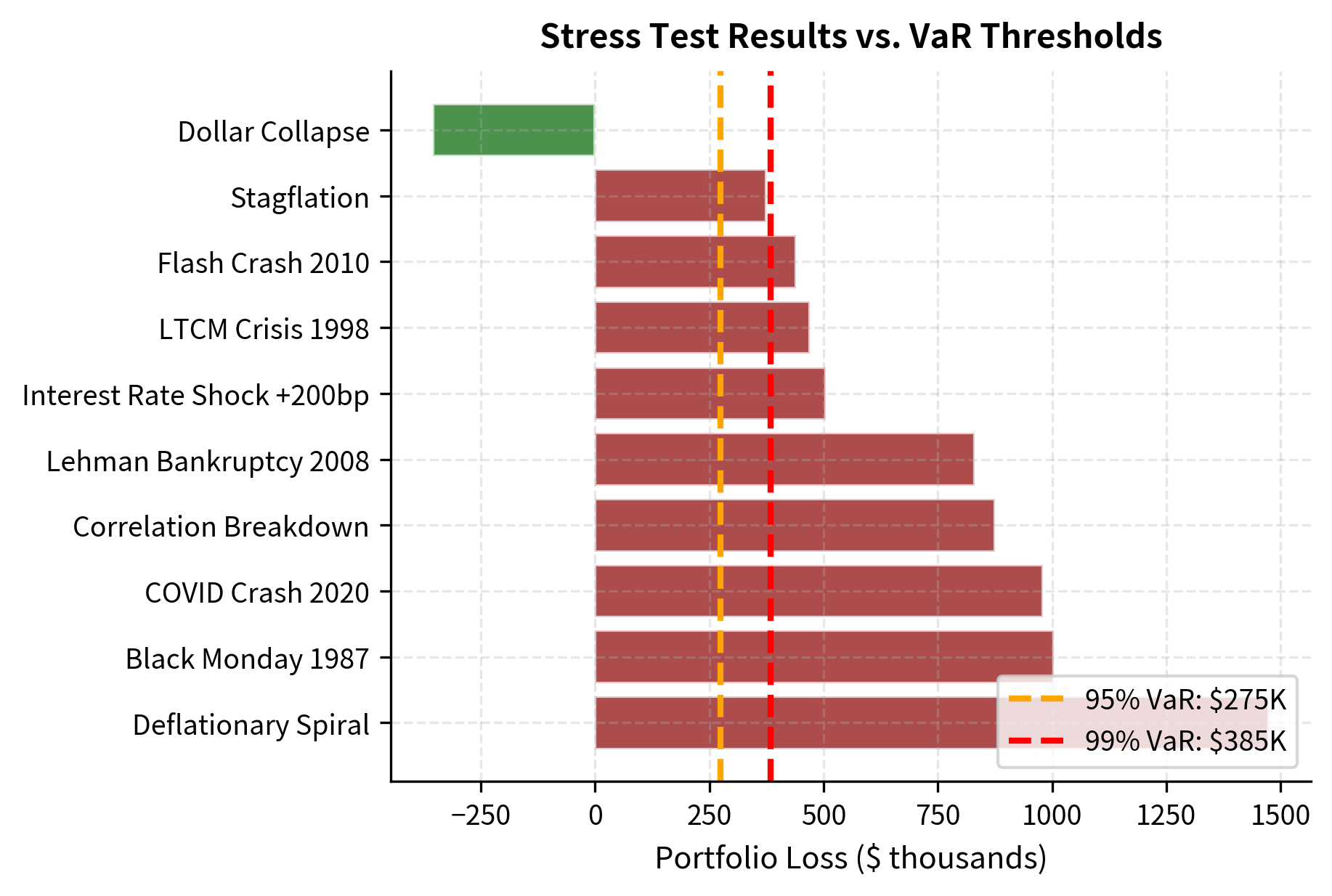
The stress test results reveal that all historical crisis scenarios produce losses substantially exceeding the 99% VaR. This is expected: VaR estimates typical tail behavior, while stress tests examine genuine market dislocations that may occur once per decade or less frequently.
Hypothetical Stress Scenarios
Beyond historical events, risk managers construct hypothetical scenarios to test vulnerabilities specific to their portfolios. These might include interest rate shocks, currency devaluations, sector-specific collapses, or combinations that stress multiple risk factors simultaneously.
The hypothetical scenarios highlight that events like a deflationary spiral or correlation breakdown could generate losses exceeding $2 million, significantly outpacing the standard VaR estimates.
Reverse Stress Testing
Traditional stress tests ask "what happens if scenario X occurs?" Reverse stress testing inverts the question: "what scenarios would cause losses exceeding threshold Y?" This helps identify hidden vulnerabilities and concentration risks.
For a portfolio heavily weighted in technology stocks, reverse stress testing might reveal that a 15% tech sector decline combined with rising interest rates would breach the firm's risk limits, even if such a scenario seems unlikely based on recent history.
Visualizing Stress Test Results
Integrating VaR, ES, and Stress Testing
Effective market risk management uses VaR, ES, and stress testing as complementary tools, not substitutes. Each provides different information essential for a complete risk picture.
VaR serves as the primary day-to-day risk metric and regulatory capital benchmark. It is computed daily, compared against limits, and used to allocate risk capital across desks and strategies. However, VaR alone is insufficient because it ignores tail severity and assumes historical patterns continue.
Expected Shortfall addresses tail severity and is increasingly mandated by regulators. The shift from 99% VaR to 97.5% ES in Basel III reflects recognition that measuring average tail losses provides more robust capital requirements.
Stress testing examines scenarios that statistical models might miss. It forces explicit consideration of "what if" questions and identifies concentration risks. Unlike VaR and ES, stress tests can incorporate forward-looking views about emerging risks not present in historical data.
Key Parameters
The market risk models implemented here rely on several key parameters:
- n_obs: The lookback window for historical simulation (504 days).
- n_simulations: The number of scenarios generated for Monte Carlo methods (10,000).
- degrees_of_freedom: The shape parameter for the t-distribution (), controlling tail heaviness.
- weights: The portfolio allocation vector across assets.
- confidence_level: The probability threshold () for VaR and ES calculations (95% or 99%).
Practical Considerations
Implementing VaR systems in production requires addressing several practical challenges beyond the mathematical framework.
Data Quality and History
VaR calculations are only as good as the underlying data. Missing prices, stale quotes, and corporate actions (splits, dividends) can introduce significant errors. Historical simulation is particularly sensitive: a data error creating a spurious extreme return will directly impact VaR estimates. Production systems require robust data validation and cleaning procedures.
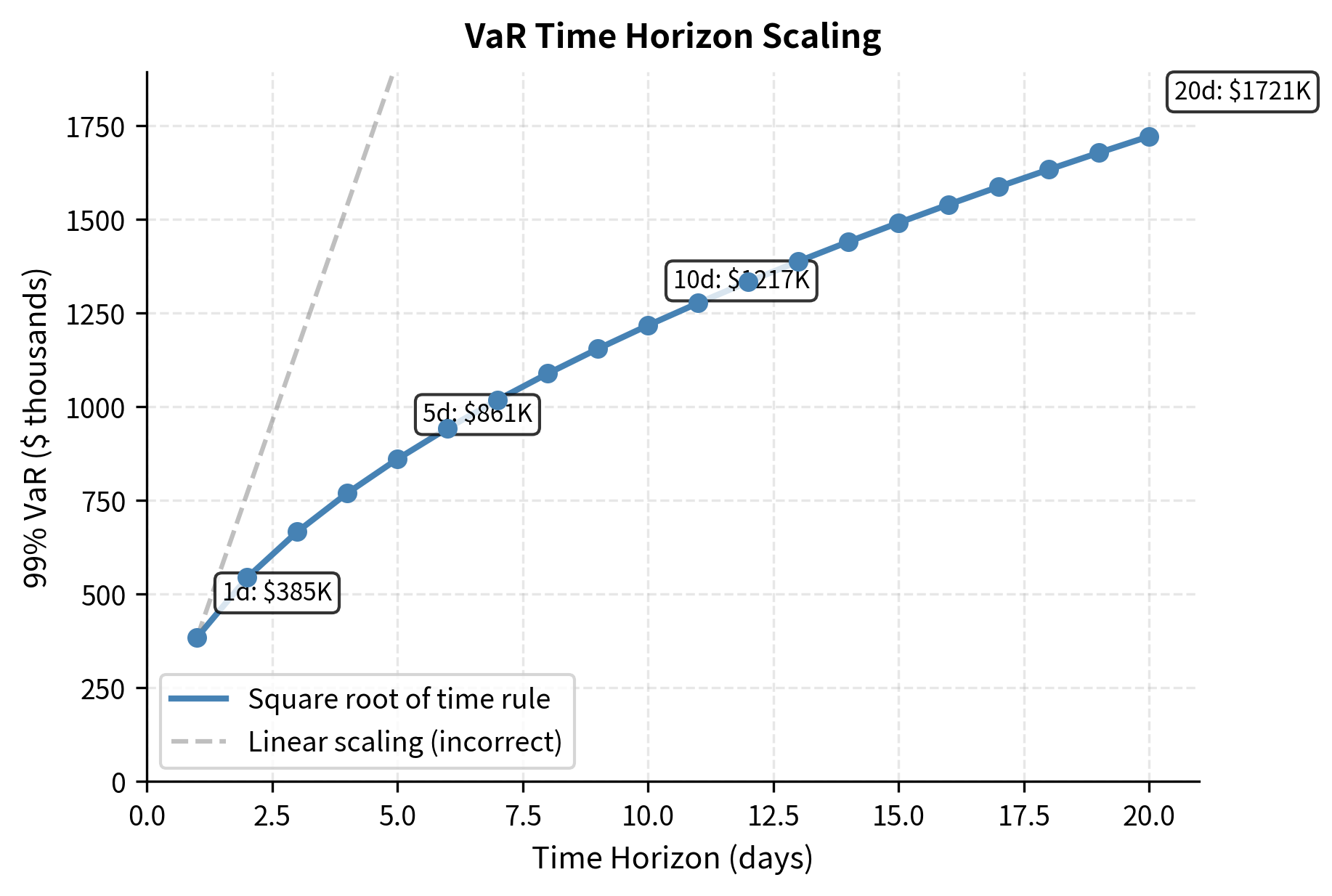
Time Horizon Scaling
Regulators often require 10-day VaR for capital calculations, but most institutions compute daily VaR internally. A common approximation scales daily VaR by where is the horizon in days:
where:
- : VaR for an -day horizon
- : VaR for a 1-day horizon
- : time horizon in days
This scaling assumes returns are independent and identically distributed, which is violated by volatility clustering. When volatility is elevated, the square-root-of-time rule underestimates multi-day risk because high volatility tends to persist.
Backtesting and Model Validation
Robust VaR systems include ongoing backtesting that compares predicted VaR to actual P&L. The Basel framework specifies a traffic light approach: too few exceedances suggest the model is overly conservative (inefficient capital usage), while too many indicate underestimation of risk and potential capital inadequacy.
A formal backtest statistic is Kupiec's proportion-of-failures test, which compares the observed exceedance rate to the expected rate under the null hypothesis of a correctly specified model:
The Kupiec test p-value indicates that we cannot reject the null hypothesis of a correct model at the 5% significance level. The observed number of exceedances is statistically consistent with the expected number given the sample size, suggesting the VaR model is calibrated correctly for this period.
The next chapter on Credit Risk Fundamentals extends our risk measurement framework from market risk to the distinct challenges of measuring and managing default and credit spread risk.
Summary
This chapter developed the three major approaches to market risk measurement and explored their limitations and extensions.
Value-at-Risk quantifies the maximum expected loss at a given confidence level and time horizon. The parametric method assumes normally distributed returns and provides fast, closed-form calculations but underestimates tail risk. Historical simulation uses actual past returns without distributional assumptions but depends heavily on the lookback window. Monte Carlo simulation offers flexibility to incorporate complex dynamics like fat tails and time-varying volatility.
VaR limitations include silence about tail severity, potential violations of sub-additivity, and dependence on historical patterns that may not persist. The 2008 financial crisis demonstrated that VaR can provide false comfort when market dynamics shift dramatically.
Expected Shortfall addresses tail severity by measuring the average loss given that VaR is exceeded. It satisfies the coherence axioms that VaR violates and has become the primary regulatory metric under Basel III.
Stress testing complements statistical measures by examining portfolio performance under extreme but plausible scenarios. Historical stress tests use actual crisis returns, while hypothetical scenarios explore vulnerabilities not present in historical data. Together, VaR, ES, and stress testing provide a comprehensive view of market risk that no single measure can deliver alone.
Quiz
Ready to test your understanding? Take this quick quiz to reinforce what you've learned about Value-at-Risk, Expected Shortfall, and stress testing methodologies.

Comments