

Master market, credit, liquidity, operational, and model risk. Learn Basel III capital requirements and risk management governance structures.
Choose your expertise level to adjust how many terms are explained. Beginners see more tooltips, experts see fewer to maintain reading flow. Hover over underlined terms for instant definitions.
Overview of Financial Risks and Regulatory Frameworks
Risk is the defining feature of financial markets. Every position, every trade, every strategic decision carries the potential for outcomes that deviate from expectations, sometimes favorably, often not. Throughout this book, you have built models to price assets, construct portfolios, and value derivatives. But models are only as useful as our ability to understand when they might fail, and portfolios are only as valuable as our capacity to survive adverse market conditions. Risk management transforms theoretical knowledge into practical survival.
The financial crisis of 2008 demonstrated with painful clarity what happens when risk management fails. Institutions that had accumulated vast exposures to mortgage-backed securities and their derivatives discovered that their models had vastly underestimated the probability of correlated defaults. Liquidity that had seemed abundant evaporated overnight. Counterparties that had appeared solvent became insolvent. The cascade of failures threatened the entire global financial system.
This chapter provides a systematic framework for understanding financial risks. We begin by categorizing the major risk types that institutions face: market risk, credit risk, liquidity risk, operational risk, and model risk. We then examine what effective risk management seeks to achieve and how regulatory frameworks, particularly the Basel Accords, shape institutional behavior. Finally, we explore how firms organize their risk management functions to identify, measure, monitor, and control these risks. This foundation prepares you for the detailed quantitative tools covered in subsequent chapters.
Categories of Financial Risk
Financial institutions face a complex web of interconnected risks. While these risks often interact and compound each other, it is analytically useful to decompose them into distinct categories. Each category requires different measurement approaches, different mitigation strategies, and different organizational responses. By understanding each risk type in isolation, we build the foundation needed to appreciate their dangerous interactions during periods of market stress.
Market Risk
Market risk is the potential for losses due to adverse movements in market prices: equity prices, interest rates, exchange rates, commodity prices, and volatility levels. This is perhaps the most intuitive form of financial risk: if you hold a portfolio of stocks and the market falls, you lose money. The directness of this relationship between price movements and profit or loss makes market risk the most visible and most frequently measured of all financial risks.
The risk of losses arising from changes in the market value of trading positions due to movements in market factors such as prices, rates, and volatilities.
To understand why market risk matters so deeply to financial institutions, consider that most trading positions are marked to market daily. This means that unrealized gains and losses flow directly through to profit and loss statements. A portfolio manager cannot simply ignore adverse price movements by refusing to sell, as the losses are recognized immediately in the accounting records. This real-time recognition of gains and losses creates both discipline and vulnerability: discipline because it forces honest assessment of position values, and vulnerability because it can trigger forced selling when losses accumulate.
Market risk manifests in several forms, each requiring distinct measurement approaches and hedging strategies:
- Equity risk: Exposure to changes in stock prices, sector indices, or broad market movements. A portfolio long technology stocks faces equity risk from both company-specific events and broader market selloffs. Equity risk can be decomposed into systematic risk, which affects all stocks and cannot be diversified away, and idiosyncratic risk, which is specific to individual companies and can be reduced through diversification.
- Interest rate risk: Exposure to changes in interest rates across different maturities. As we discussed in Part II on bond risk measures, a portfolio of fixed-income securities loses value when rates rise. The relationship between bond prices and interest rates is governed by duration and convexity, metrics that allow us to quantify and hedge this exposure.
- Currency risk: Exposure to changes in foreign exchange rates. An American firm with European revenues faces losses when the euro depreciates against the dollar. Currency risk affects not only explicit foreign exchange positions but also any asset whose value is denominated in a foreign currency.
- Commodity risk: Exposure to changes in commodity prices. An airline faces commodity risk from jet fuel prices; a mining company faces it from metal prices. Commodity risk is particularly challenging because commodity prices often exhibit different statistical properties than financial assets, including seasonality and the potential for supply disruptions.
- Volatility risk: Exposure to changes in implied or realized volatility. As we explored in Part III on the Greeks, option portfolios have significant vega exposure: their values change as volatility expectations shift. Volatility risk is unique in that volatility itself is not directly tradeable; it must be accessed through derivatives whose prices depend on volatility.
Market risk is typically the dominant concern for trading operations. A prop trading firm running a statistical arbitrage strategy, a market maker providing liquidity in options, or a hedge fund implementing momentum strategies all face market risk as their primary threat. The tools we develop in subsequent chapters, particularly Value at Risk and Expected Shortfall, are designed primarily to measure and manage this category of risk.
To illustrate market risk dynamics and the benefits of diversification, the following code simulates a portfolio composed of equities, bonds, and currencies.
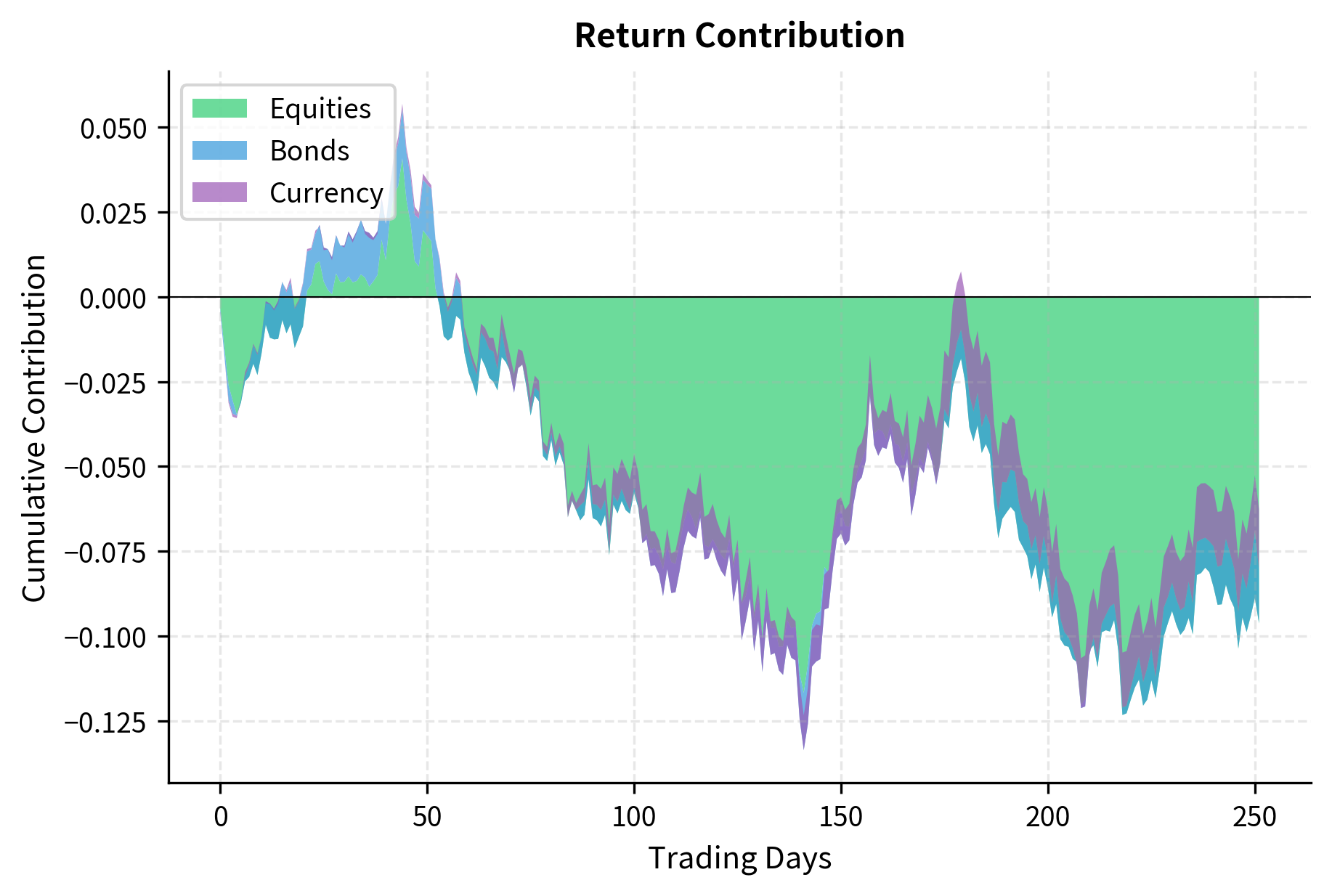
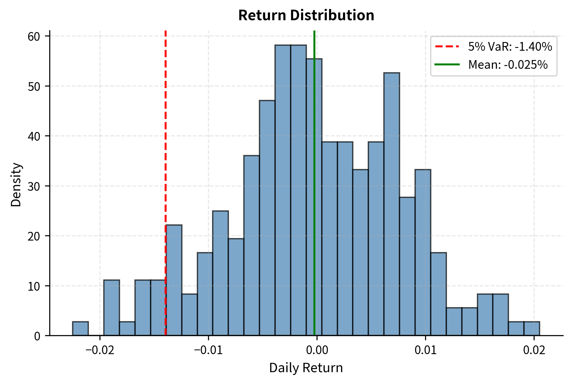
The cumulative contribution plot shows how different asset classes contribute to portfolio returns over time, illustrating the diversification benefit of holding multiple asset types. Notice how the contributions from different asset classes sometimes offset each other: when equities underperform, bonds may provide stability, reducing overall portfolio volatility. The return distribution plot shows the distribution of daily returns, with the red dashed line indicating the 5th percentile, a crude measure of daily risk that we will refine significantly in the next chapter on Value at Risk.
Key Parameters
The simulation relies on the following parameters, each of which captures an essential aspect of market risk:
- mu: Vector of expected daily returns for each asset class. These represent our assumptions about the average return we expect from each asset type over time. Equities have the highest expected return (8% annualized), reflecting the equity risk premium, while bonds and currency have lower expected returns.
- cov_annual: Annualized covariance matrix capturing the risk and co-movement of assets. The diagonal elements represent each asset's variance, or the square of its volatility, while the off-diagonal elements represent covariances that determine how assets move together. Lower covariances between asset classes provide diversification benefits.
- weights: Allocation of capital to each asset class (60% Equities, 30% Bonds, 10% Currency). These weights determine how much each asset's returns contribute to the overall portfolio. A higher weight on volatile assets increases portfolio risk, while diversifying across assets with low correlations reduces it.
Credit Risk
Credit risk is the potential for losses due to a counterparty's failure to meet its contractual obligations. When you lend money, the borrower might default. When you enter a derivatives contract, your counterparty might fail to make required payments. Unlike market risk, where losses occur because prices move against you, credit risk involves the more fundamental problem of not receiving money you are owed.
The risk of loss arising from a borrower or counterparty failing to meet their financial obligations, including both default and deterioration in credit quality.
The distinction between market risk and credit risk is subtle but important. With market risk, you face potential losses even when all parties honor their obligations: a bond might fall in price simply because interest rates rise. With credit risk, the loss arises specifically from a failure to perform. However, these risks interact: a bond's price might fall because the market perceives increased default probability, blending credit spread risk with pure credit default risk.
Credit risk takes several forms, each with distinct characteristics and measurement challenges:
- Default risk: The outright failure of a counterparty to make required payments. A bondholder faces default risk if the issuing company goes bankrupt. Default is a discrete event, either it happens or it doesn't, which makes it fundamentally different from the continuous price movements of market risk.
- Credit spread risk: Changes in the market's assessment of creditworthiness, even absent actual default. If a company's credit rating is downgraded, its bond prices fall as spreads widen. This is sometimes called "migration risk" because it relates to the borrower migrating between credit quality categories.
- Recovery risk: Uncertainty about the amount recovered in the event of default. Even knowing that a company will default, the bondholder faces uncertainty about how much they will eventually receive. Recovery rates vary widely depending on the seniority of the debt, the assets available for liquidation, and the complexity of bankruptcy proceedings.
- Counterparty credit risk: The risk that a derivative counterparty defaults when the position has positive value to you. This was a central concern during the 2008 crisis, particularly around credit default swaps. Counterparty risk is particularly complex because your exposure changes with market movements, creating "wrong-way risk" when a counterparty's credit quality deteriorates precisely when your exposure to them increases.
As we discussed in Part II on credit default swaps and structured credit products, the instruments designed to transfer credit risk can themselves become sources of systemic risk when correlations between default events are underestimated.
The quantitative foundation of credit risk is the Expected Loss () metric, which decomposes the complex phenomenon of potential credit losses into three measurable components. This decomposition is both conceptually elegant and practically useful because it separates the question "how likely is loss?" from "how much will we lose if it happens?" and "how much do we have at stake?" The formula is:
To understand why this formula takes this form, consider what we need to know to estimate our expected credit loss. First, we need to know the probability that a loss will occur at all, which is the Probability of Default (). A loan to a highly creditworthy borrower might have a PD of 0.1%, while a loan to a troubled company might have a PD of 10%. Second, if default occurs, we need to know what fraction of our exposure we will actually lose, which is the Loss Given Default (). This is calculated as , where the recovery rate represents the percentage of the loan we expect to eventually collect through bankruptcy proceedings, collateral liquidation, or restructuring. Finally, we need to know how much we have at stake when the default occurs, which is the Exposure at Default (). For a term loan, this is simply the outstanding principal, but for credit lines or derivatives, the exposure may be uncertain and require modeling.
The components of the Expected Loss formula are:
- : Probability of Default, the likelihood that the borrower fails to pay. This is typically estimated from historical default rates for borrowers with similar credit ratings, or from market data such as credit default swap spreads.
- : Loss Given Default, the percentage of exposure lost if default occurs (). Recovery rates vary significantly by industry, collateral type, and position in the capital structure. Senior secured loans typically have higher recovery rates than subordinated debt.
- : Exposure at Default, the total value at risk at the time of default. For drawn loans, this equals the outstanding balance. For undrawn commitments, it requires estimating how much the borrower will draw before defaulting.
The following example calculates Expected Loss for a hypothetical loan portfolio using these components.
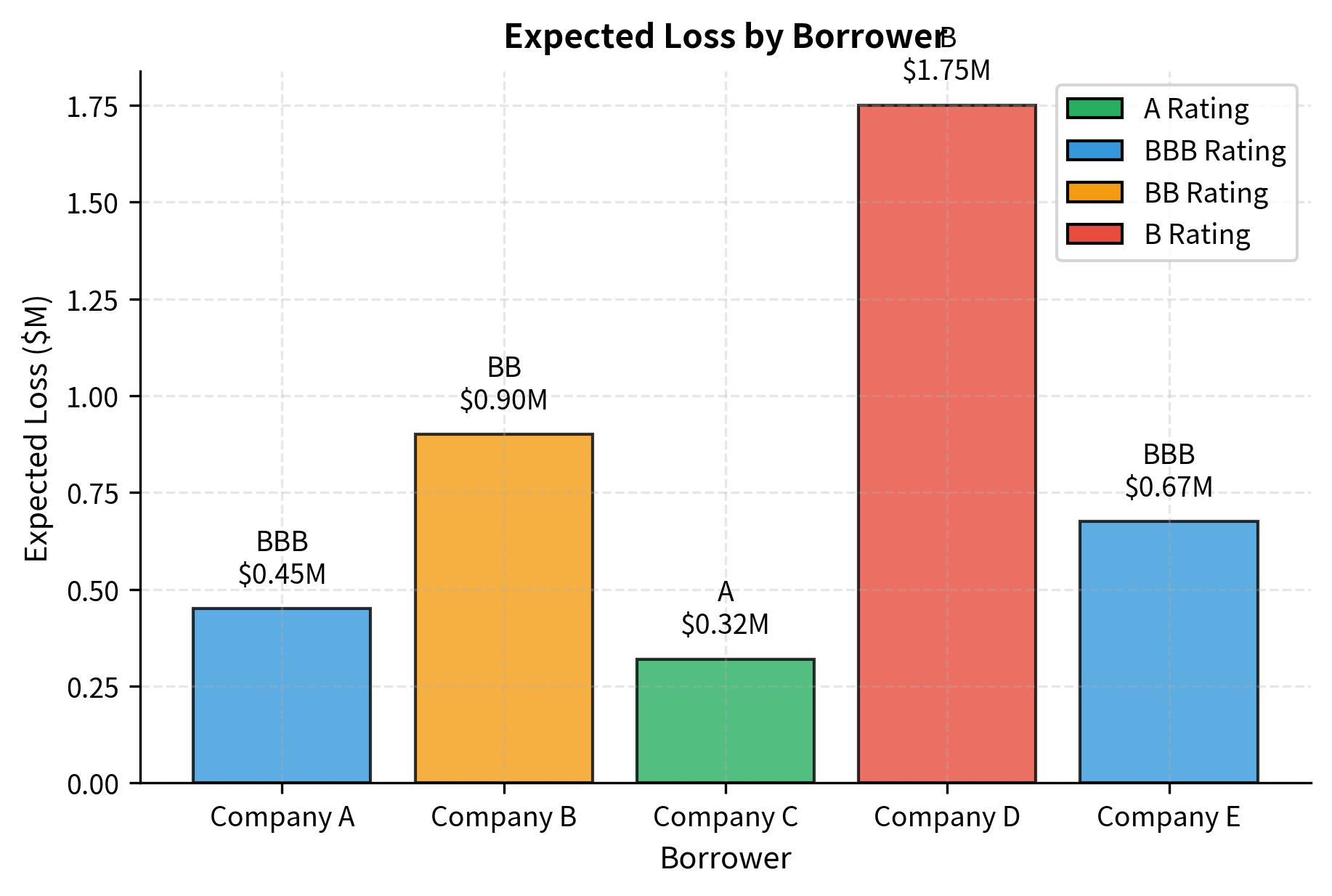
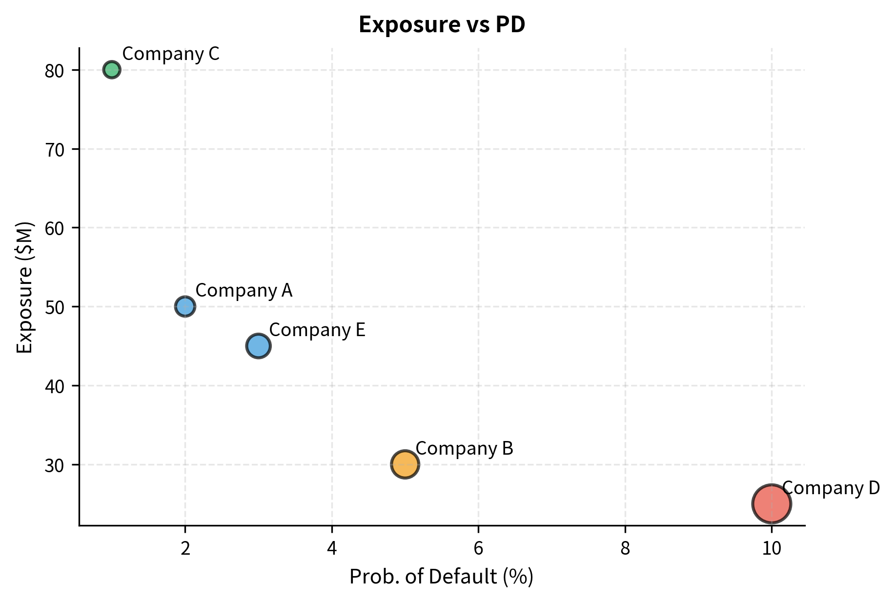
This simple expected loss calculation illustrates the three key components of credit risk measurement: the exposure at default (how much you could lose), the probability of default (how likely loss is), and loss given default (what fraction you lose if default occurs). Notice how Company D, despite having the smallest exposure, contributes meaningfully to portfolio expected loss because of its high probability of default and high loss given default. This demonstrates why risk management cannot focus solely on exposure size; the credit quality of borrowers matters enormously. We will develop much more sophisticated credit risk models in the upcoming chapters on credit risk fundamentals and modeling approaches.
Key Parameters
The key parameters for the Expected Loss model each serve a distinct purpose in quantifying credit risk:
- PD: Probability of Default. The likelihood that a borrower defaults over a given time horizon, typically one year. PD is usually estimated from historical default rates by credit rating, from statistical models (such as Merton's structural model or logistic regression), or inferred from market prices like credit default swap spreads.
- LGD: Loss Given Default. The fraction of exposure lost if a default occurs, calculated as (1 - Recovery Rate). LGD depends on factors such as collateral quality, seniority of the claim, industry characteristics, and the economic environment at the time of default. Secured loans typically have LGDs of 30-50%, while subordinated unsecured debt may have LGDs of 70-90%.
- Exposure_M: Exposure at Default (EAD). The total value exposed to credit loss at the time of default (in millions). For term loans, EAD equals the outstanding balance. For revolving credit facilities, EAD must account for additional draws that borrowers typically make as they approach default.
Liquidity Risk
Liquidity risk is the potential for losses arising from the inability to meet payment obligations or to exit positions without incurring unacceptable costs. Unlike market risk, which relates to price movements, liquidity risk relates to the ability to transact at reasonable prices, or to transact at all. An asset might have a well-defined market price, but if you cannot sell it at that price when you need to, the quoted price provides little comfort.
The risk that a firm cannot meet its short-term financial demands (funding liquidity) or cannot exit positions without significantly affecting market prices (market liquidity).
Liquidity risk is often described as a "meta-risk" because it amplifies other risks. A position that would be manageable if you could exit it becomes dangerous when exit is impossible or prohibitively expensive. This amplification effect means that liquidity considerations should infuse all aspects of risk management, not exist as a separate category considered in isolation.
Liquidity risk has two distinct but related dimensions:
- Funding liquidity risk: The risk that a firm cannot meet its payment obligations when due, whether through cash, borrowing, or asset sales. A firm might be solvent on a mark-to-market basis but still face a liquidity crisis if it cannot roll over short-term debt. The classic example is a bank run: depositors demanding withdrawal simultaneously forces the bank to liquidate assets at fire-sale prices, potentially causing insolvency even if the bank was initially solvent.
- Market liquidity risk: The risk that a firm cannot exit positions without moving the market price significantly against itself. A fund holding large positions in small-cap stocks may find that selling quickly requires accepting substantial price discounts. Market liquidity risk increases with position size relative to typical trading volume and varies dramatically across asset classes and market conditions.
These two forms of liquidity risk can interact dangerously, creating what economists call a "liquidity spiral." In a crisis, funding becomes scarce precisely when assets become illiquid. Institutions forced to sell illiquid assets to meet margin calls push prices down further, triggering more margin calls and more forced selling, creating a feedback loop that amplifies market dislocations far beyond what fundamentals would justify.
We can visualize the liquidity spectrum by comparing bid-ask spreads and liquidation times across different asset classes.
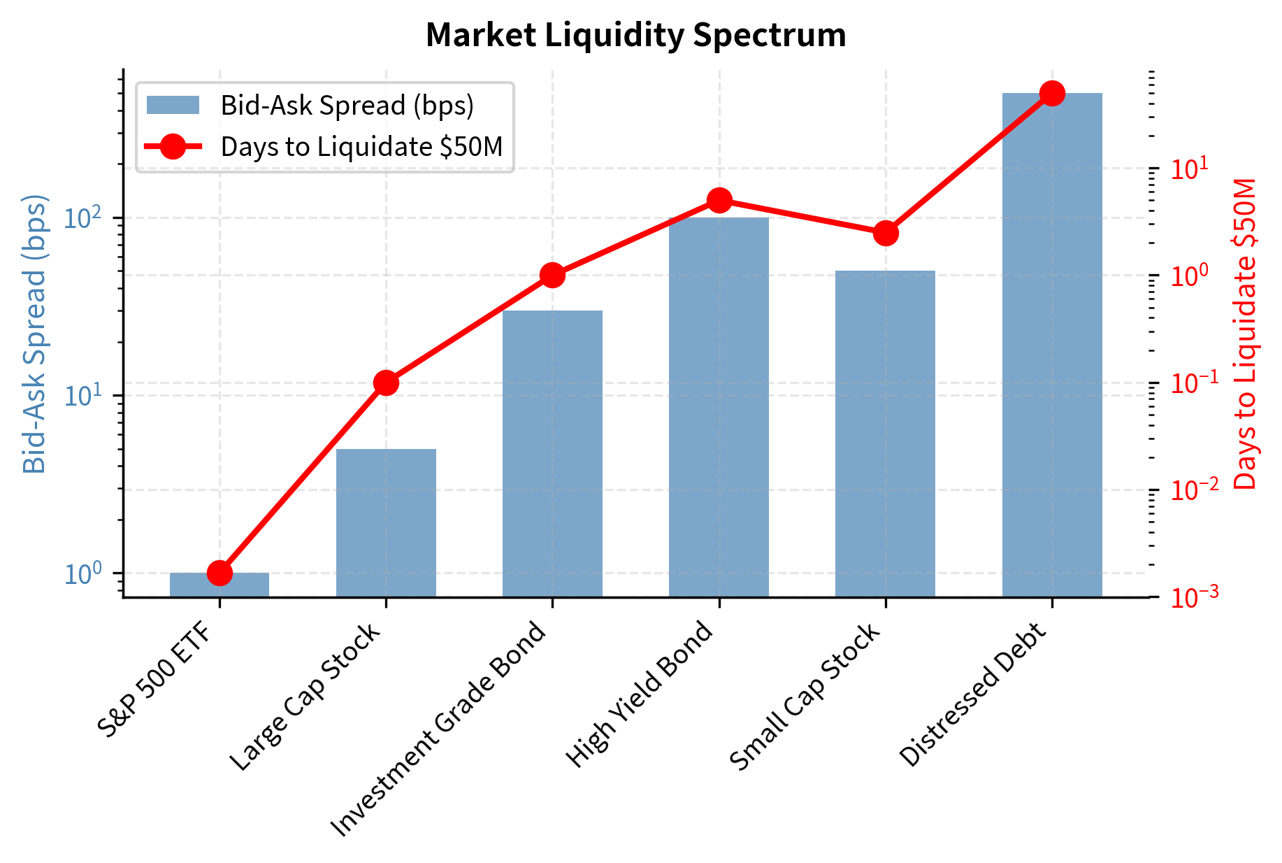
The dramatic variation in liquidity across asset classes has profound implications for portfolio management and risk measurement. A \$50 million portfolio of S&P 500 ETFs can be liquidated in minutes with minimal market impact. The same capital deployed in distressed debt might take months to exit with significant price concessions required. This variation means that traditional risk measures like Value at Risk, which assume positions can be liquidated at current market prices, may substantially understate true risk for illiquid portfolios.
Key Parameters
The liquidity analysis uses three complementary metrics to capture different aspects of market liquidity:
- Bid_Ask_bps: The bid-ask spread in basis points, representing the immediate cost of trading. This is the difference between the price at which you can buy (the ask) and the price at which you can sell (the bid), expressed as a fraction of the mid-price. Wider spreads indicate higher trading costs and typically correlate with lower market liquidity.
- Daily_Volume_M: Average daily trading volume in millions, indicating market depth. Higher volumes suggest that large trades can be absorbed without significant price impact. However, volume alone can be misleading; you must also consider how your trade size compares to typical volume.
- Days_to_Liquidate_50M: Estimated days required to exit a \$50M position calculated based on volume participation limits. This metric assumes you cannot capture more than a certain fraction (often 10-25%) of daily volume without significantly moving the price. For illiquid assets, this constraint means that large positions may take weeks or months to unwind.
Operational Risk
Operational risk is the potential for losses arising from inadequate or failed internal processes, people, systems, or external events. This catch-all category encompasses everything from trading errors to cyber attacks to natural disasters.
The risk of loss resulting from inadequate or failed internal processes, people, and systems, or from external events. This includes legal risk but excludes strategic and reputational risk.
Operational risk events vary enormously in nature and severity:
- Process failures: Settlement errors, incorrect trade entries, failed reconciliations, missed deadlines
- People failures: Rogue trading, fraud, key person departures, inadequate training
- System failures: IT outages, data corruption, algorithmic malfunctions, cybersecurity breaches
- External events: Natural disasters, terrorism, regulatory changes, pandemic disruptions
Unlike market and credit risk, operational risk is notoriously difficult to quantify. Market risk can be estimated from price histories; credit risk can be inferred from default rates and spreads. Operational risk events are often rare, idiosyncratic, and potentially catastrophic; a single rogue trader can destroy an institution.
Historical examples illustrate the stakes:
- Barings Bank (1995): Nick Leeson's unauthorized trading losses of £827 million destroyed the 233-year-old bank
- Knight Capital (2012): A software deployment error caused \$440 million in losses in 45 minutes
- LTCM (1998): While primarily a market risk event, operational failures in risk management contributed to the near-collapse that threatened systemic stability
The Basel framework requires banks to hold capital against operational risk, but the measurement challenge means that approaches range from simple revenue-based formulas to complex internal models using loss data and scenario analysis.
Model Risk
Model risk is the potential for adverse consequences arising from decisions based on incorrect or misused models. As quantitative methods have become central to finance, model risk has emerged as a distinct category worthy of dedicated attention. Nearly every risk measure, valuation, and trading decision in modern finance depends on models, making model risk a pervasive concern that touches all other risk categories.
The risk of loss arising from the use of models that are fundamentally flawed, incorrectly implemented, or inappropriately applied in decision-making.
Understanding model risk requires appreciating the distinction between a model and reality. A model is a simplified representation that captures some aspects of the world while ignoring others. The Black-Scholes model, for example, captures the relationship between option prices and key variables like underlying price, volatility, and time to expiration, but it ignores features of real markets like jumps, stochastic volatility, and transaction costs. Whether these simplifications matter depends on how the model is used and what questions it is asked to answer.
Model risk manifests through several channels, each requiring different mitigation approaches:
- Specification error: The model makes incorrect assumptions about the underlying process. The Black-Scholes model assumes constant volatility; the real world exhibits volatility clustering and jumps. Specification error is particularly dangerous when it leads to systematic underestimation of tail risks.
- Estimation error: Parameters are estimated with error from limited data. A volatility estimate from 252 daily returns has substantial sampling uncertainty. Even a perfectly specified model will produce imprecise outputs if its parameters cannot be estimated precisely.
- Implementation error: The model is coded incorrectly. A sign error in a delta-hedging algorithm can turn a hedge into a doubled position. Implementation errors can lurk undetected for years before manifesting during unusual market conditions.
- Application error: A model is used outside its domain of validity. A model calibrated to normal market conditions may fail spectacularly in a crisis. Application error often occurs when models developed for one purpose are repurposed for another without adequate testing.
Throughout Part III on derivatives pricing and Part IV on portfolio construction, we developed models that make specific assumptions. The Black-Scholes framework assumes geometric Brownian motion with constant volatility. Mean-variance optimization assumes returns are fully characterized by their first two moments. Factor models assume linear relationships. In each case, reality diverges from these assumptions, and understanding how that divergence affects model outputs is essential.
To demonstrate model risk, we will simulate the impact of volatility estimation error on Black-Scholes option prices. This example focuses on estimation error: even when the model structure is correct, limited data creates meaningful uncertainty in parameter estimates, which propagates through to uncertainty in model outputs.
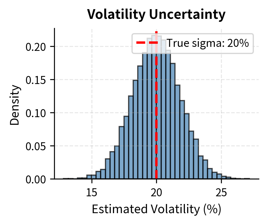
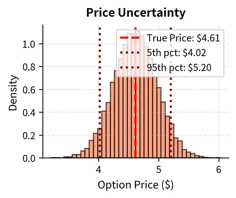
This example demonstrates that even when the model structure is correct, parameter uncertainty creates meaningful price uncertainty. The fundamental challenge is that we never observe the true volatility directly; we must estimate it from a finite sample of historical returns. This estimation introduces error that propagates through to our option prices.
The precision of a volatility estimate depends on the sample size according to the standard error formula:
To understand why this formula takes this form, consider the intuition: volatility is estimated from the variance of returns, and sample variances have well-known statistical properties. The denominator contains because, like most statistical estimators, precision improves with the square root of sample size. The factor of 2 in the denominator arises from the specific statistical properties of the chi-squared distribution that governs sample variance estimation.
The components of the standard error formula are:
- : standard error of the volatility estimator, representing the typical magnitude of our estimation error
- : true volatility, which unfortunately must itself be estimated or assumed
- : number of observations in the sample, typically the number of daily returns used in estimation
A volatility estimate based on 60 trading days (roughly three months) has a standard error of roughly 1.8 percentage points. This means that if true volatility is 20%, our estimate might plausibly be anywhere from 16% to 24%. Since option prices are approximately linear in volatility for at-the-money options, this volatility uncertainty translates directly to the significant option price uncertainty shown in the summary statistics above. A trader who ignores this model risk might believe they know an option's fair value to within pennies when the true uncertainty is measured in dollars.
Key Parameters
The Black-Scholes model used in this illustration relies on the following parameters, each of which must either be observed directly or estimated:
- S: Current stock price ($100) This is directly observable from market data and introduces no estimation error.
- K: Strike price ($100) This is a contractual term that is known exactly.
- T: Time to expiration (0.25 years). This is calculable from contract specifications, though subtleties arise around day count conventions.
- r: Risk-free interest rate (5%). This must be estimated, typically from Treasury yields, and introduces some uncertainty, though generally less than volatility.
- sigma: Volatility of the underlying asset. In this simulation, we treat this as an estimated parameter with uncertainty. This is the dominant source of model risk for option pricing because volatility is not directly observable and must be inferred from historical data or implied from market prices.
Objectives of Risk Management
Understanding the types of risk is necessary but not sufficient. We must also understand what risk management seeks to achieve. Risk management is not about eliminating risk, as that would eliminate returns as well. Rather, it is about taking risks intelligently, ensuring that the risks taken are understood, intentional, and appropriately compensated.
Protecting Capital
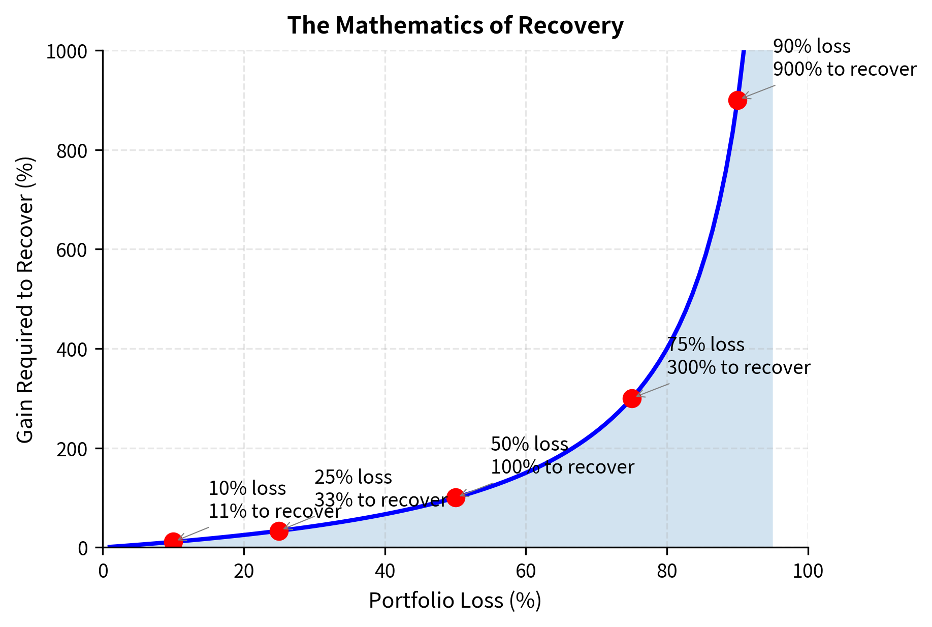
The fundamental objective of risk management is survival. A trading firm or fund can recover from a bad year, but it cannot recover from insolvency. This asymmetry (the profound difference between a 50% loss and extinction) shapes everything about how risk management must be approached.
Consider the mathematics of recovery. A 50% loss requires a 100% gain to recover. A 90% loss requires a 900% gain. At some point, losses become unrecoverable not because recovery is mathematically impossible but because the time required exceeds practical horizons, or the risk-taking required to generate such returns makes another catastrophic loss even more likely.
The Kelly criterion, which optimizes long-term geometric growth, provides a theoretical foundation for this perspective. Overbetting, taking more risk than the Kelly fraction, actually reduces long-term wealth growth despite increasing expected single-period returns. The expected utility framework reaches similar conclusions: with plausible risk aversion, avoiding catastrophic losses dominates maximizing expected returns.
Ensuring Solvency Through Tail Events
Risk management must protect against tail events, the rare but extreme outcomes that lie far from normal expectations. Financial returns, as we discussed in Part III on stylized facts, exhibit fat tails: extreme events occur much more frequently than a normal distribution would suggest.
A "6-sigma" event under the normal distribution should occur roughly once every 1.5 million years. In financial markets, such moves happen every few years. Black Monday (1987), the Asian financial crisis (1997), the Russian default (1998), the dot-com crash (2000), the global financial crisis (2008), the COVID crash (2020). Each featured daily moves that should have been virtually impossible under normal assumptions.
Risk management must therefore:
- Use fat-tailed distributions or stress scenarios rather than relying solely on normal-based measures
- Implement position limits and stop-losses that prevent any single event from threatening solvency
- Maintain adequate capital buffers to absorb unexpected losses
- Plan for correlations to spike during crises (diversification fails when you need it most)
Regulatory Compliance
For regulated institutions, such as banks, broker-dealers, and insurance companies, risk management must satisfy regulatory requirements. These requirements serve both microprudential objectives (ensuring individual institution soundness) and macroprudential objectives (ensuring systemic stability).
Regulatory compliance typically requires:
- Maintaining minimum capital ratios based on risk-weighted assets
- Holding liquid asset buffers against potential outflows
- Reporting risk exposures to regulators
- Implementing governance structures with independent risk oversight
- Conducting stress tests under regulator-specified scenarios
Even unregulated entities like hedge funds face indirect regulatory pressure through their relationships with prime brokers and counterparties, who themselves face regulatory requirements around counterparty credit risk.
Optimizing Risk-Adjusted Returns
Beyond survival and compliance, risk management should help optimize risk-adjusted performance. This means:
- Allocating risk budget to strategies and positions with the highest expected Sharpe ratios
- Avoiding uncompensated risks through hedging or position adjustment
- Identifying situations where risk/reward is asymmetric in your favor
- Maintaining consistent risk levels rather than allowing risk to fluctuate with market conditions
The risk management function should not simply veto trades; it should help the firm take better trades by providing accurate risk assessment and ensuring that risk-taking is intentional rather than accidental.
Regulatory Frameworks
Financial regulation has evolved dramatically since the 2008 crisis. While the details vary by jurisdiction and institution type, the Basel framework provides the global template for bank regulation and influences risk management practices throughout the financial industry.
The Basel Accords
The Basel Committee on Banking Supervision has issued a series of accords that establish international standards for bank capital adequacy:
- Basel I (1988): Established minimum capital requirements based on risk-weighted assets, primarily focused on credit risk
- Basel II (2004): Introduced more sophisticated risk weights, incorporated operational risk, and allowed internal models for capital calculation
- Basel III (2010-2017): Substantially increased capital requirements, introduced leverage ratios, and added liquidity requirements in response to the 2008 crisis
The central concept underlying these accords is the idea of risk-weighted assets (RWA). Rather than requiring banks to hold capital against their total assets, regulators require capital against assets weighted by their riskiness. This approach serves two purposes: it ensures that riskier activities require more capital cushion, and it provides incentives for banks to shift toward safer activities.
The following code calculates risk-weighted assets (RWA) for a simplified bank balance sheet based on Basel-style asset categories.
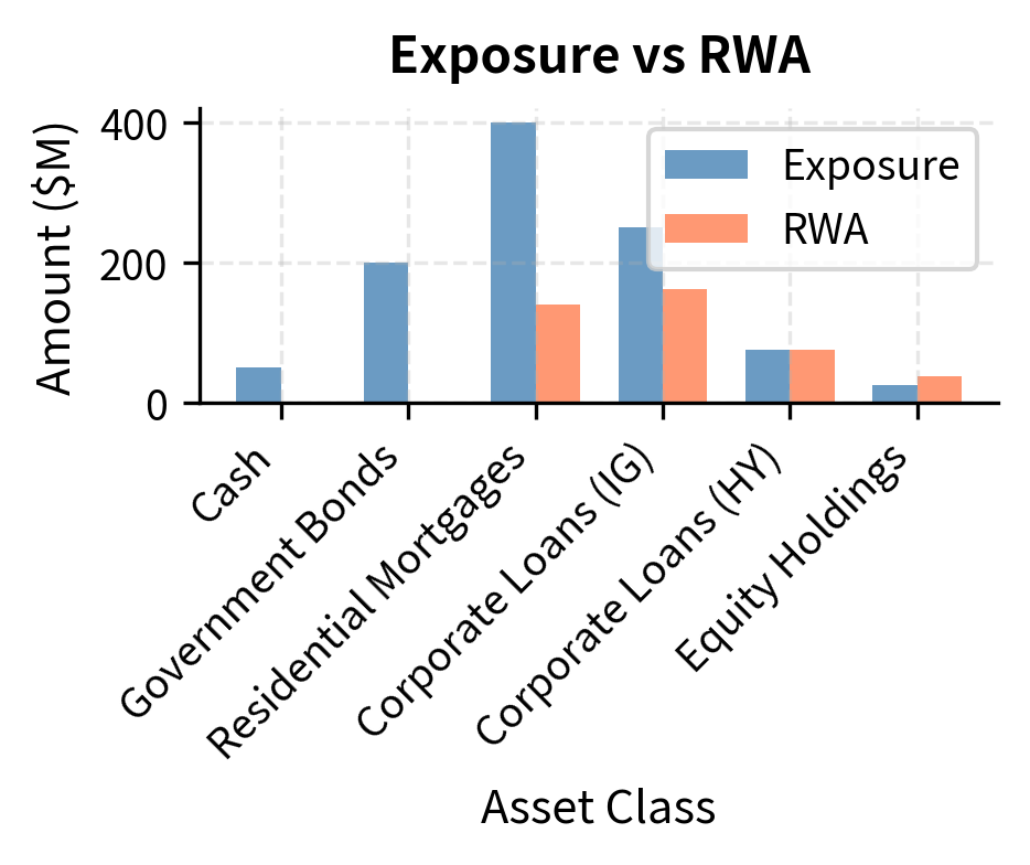
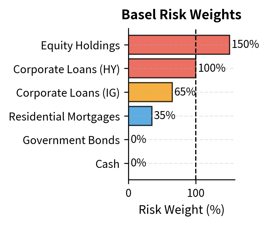
This simplified example shows how risk weights convert a $1,000 million balance sheet into $415 million of risk-weighted assets. The regulatory capital requirement applies to RWA, not total assets, which means riskier portfolios require proportionally more capital. Notice how cash and government bonds carry zero risk weight, reflecting their presumed safety, while equity holdings carry a 150% risk weight, reflecting their higher volatility and loss potential.
Key Parameters
The key parameters for the Basel RWA calculation each capture regulatory judgments about relative riskiness:
- Exposure: The nominal value of the asset on the balance sheet. This represents the maximum amount the bank could lose if the asset became worthless.
- Risk Weight: A percentage factor assigned by regulators reflecting the asset's credit risk (e.g., 0% for cash, 100% for standard corporate loans). Risk weights are set based on historical loss experience, regulatory judgment, and policy objectives. Higher risk weights effectively increase the cost of holding certain assets by requiring more capital backing.
- RWA: Risk-Weighted Assets, calculated as Exposure × Risk Weight. This is the key metric for capital adequacy: banks must hold capital equal to a minimum percentage of their RWA.
Capital Requirements Under Basel III
Basel III substantially strengthened capital requirements in both quantity and quality:
Minimum capital ratios:
| Capital Type | Minimum Requirement |
|---|---|
| Common Equity Tier 1 (CET1) | 4.5% of RWA |
| Tier 1 Capital | 6.0% of RWA |
| Total Capital | 8.0% of RWA |
| Capital Conservation Buffer | 2.5% of RWA |
| Total with Buffer | 10.5% of RWA |
Additional requirements:
- Countercyclical buffer: 0-2.5% additional CET1, set by national regulators based on credit conditions
- Systemic risk buffer: Additional requirements for globally systemically important banks (G-SIBs)
- Leverage ratio: Minimum 3% Tier 1 capital to total exposure (not risk-weighted)
Liquidity Requirements
Basel III introduced two key liquidity metrics designed to ensure banks can survive short-term stress and maintain stable funding over longer horizons:
-
Liquidity Coverage Ratio (LCR): Banks must hold high-quality liquid assets (HQLA) sufficient to cover 30 days of net cash outflows under a stress scenario. The minimum LCR is 100%. This requirement ensures that banks can survive a month-long liquidity crisis without requiring central bank intervention.
-
Net Stable Funding Ratio (NSFR): Banks must maintain stable funding (capital and long-term liabilities) sufficient to cover illiquid assets and potential contingent claims over a one-year horizon. The minimum NSFR is 100%. This requirement addresses maturity mismatch, discouraging banks from funding long-term illiquid assets with short-term volatile funding.
We can calculate the Liquidity Coverage Ratio (LCR) for a bank using the following components. The LCR is defined as the ratio of high-quality liquid assets to net cash outflows over a 30-day stress period:
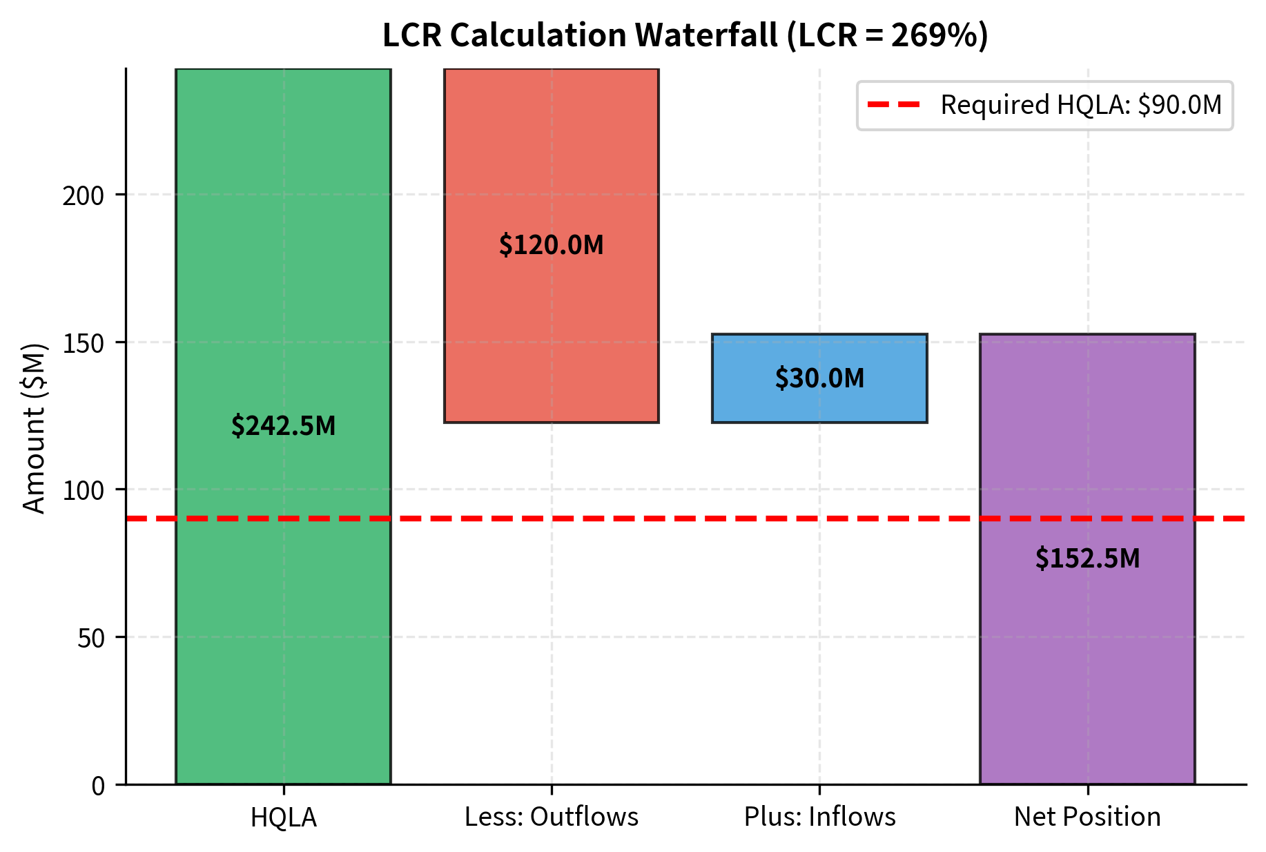
The LCR calculation results in a ratio well above the 100% threshold, indicating that the bank's high-quality liquid assets are sufficient to cover the projected net cash outflows under stress. The various run-off rates (5% for retail deposits, 25% for wholesale deposits) reflect regulatory assumptions about how quickly different funding sources might flee during a crisis. Retail deposits are considered more stable because they are typically insured and held by less sophisticated depositors, while wholesale deposits are considered more flight-prone.
Key Parameters
The key parameters for the Liquidity Coverage Ratio each reflect regulatory judgments about asset quality and liability stability:
- HQLA: High-Quality Liquid Assets. Assets that can be easily and immediately converted into cash at little or no loss of value. Central bank reserves and government securities receive 100% credit, while lower-quality assets face haircuts reflecting potential value loss under stress conditions.
- Net Cash Outflows: Total expected cash outflows minus total expected cash inflows (subject to a cap) over a 30-day stress period. The outflow assumptions are conservative, reflecting crisis conditions when depositors may flee and credit commitments may be drawn. Inflows are capped to prevent banks from relying too heavily on uncertain cash sources.
- LCR: The ratio of HQLA to Net Cash Outflows. Must be at least 100%, meaning the bank must hold enough liquid assets to cover all expected net outflows for 30 days without any additional funding.
Implications for Non-Bank Entities
While Basel regulations apply directly only to banks, they influence the entire financial ecosystem:
- Hedge funds face margin requirements and collateral demands from their prime brokers, who must account for counterparty credit risk in their regulatory capital
- Asset managers face liquidity requirements ensuring they can meet redemption requests
- Clearing houses face capital and liquidity requirements designed to ensure they can absorb member defaults
- Proprietary trading firms may face less direct regulation but impose internal risk limits analogous to regulatory requirements
Even unregulated entities benefit from understanding regulatory frameworks, as these shape counterparty behavior, market structure, and systemic risk dynamics.
Risk Management Organization and Governance
Effective risk management requires more than quantitative tools; it requires organizational structures that identify, measure, monitor, and control risks. A well-designed risk governance framework ensures that risk-taking is intentional, understood, and appropriately limited.
The Three Lines of Defense
Most financial institutions organize risk management around a "three lines of defense" model. This framework creates a hierarchy of risk ownership, oversight, and assurance, ensuring that multiple layers of protection exist against excessive risk-taking. The first line consists of business units who own and manage risk in their daily activities. The second line consists of risk management and compliance functions that provide independent oversight and challenge to the first line. The third line consists of internal audit, which provides independent assurance that both the first and second lines are functioning as designed. This layered structure ensures that no single failure point can compromise the entire risk management system.
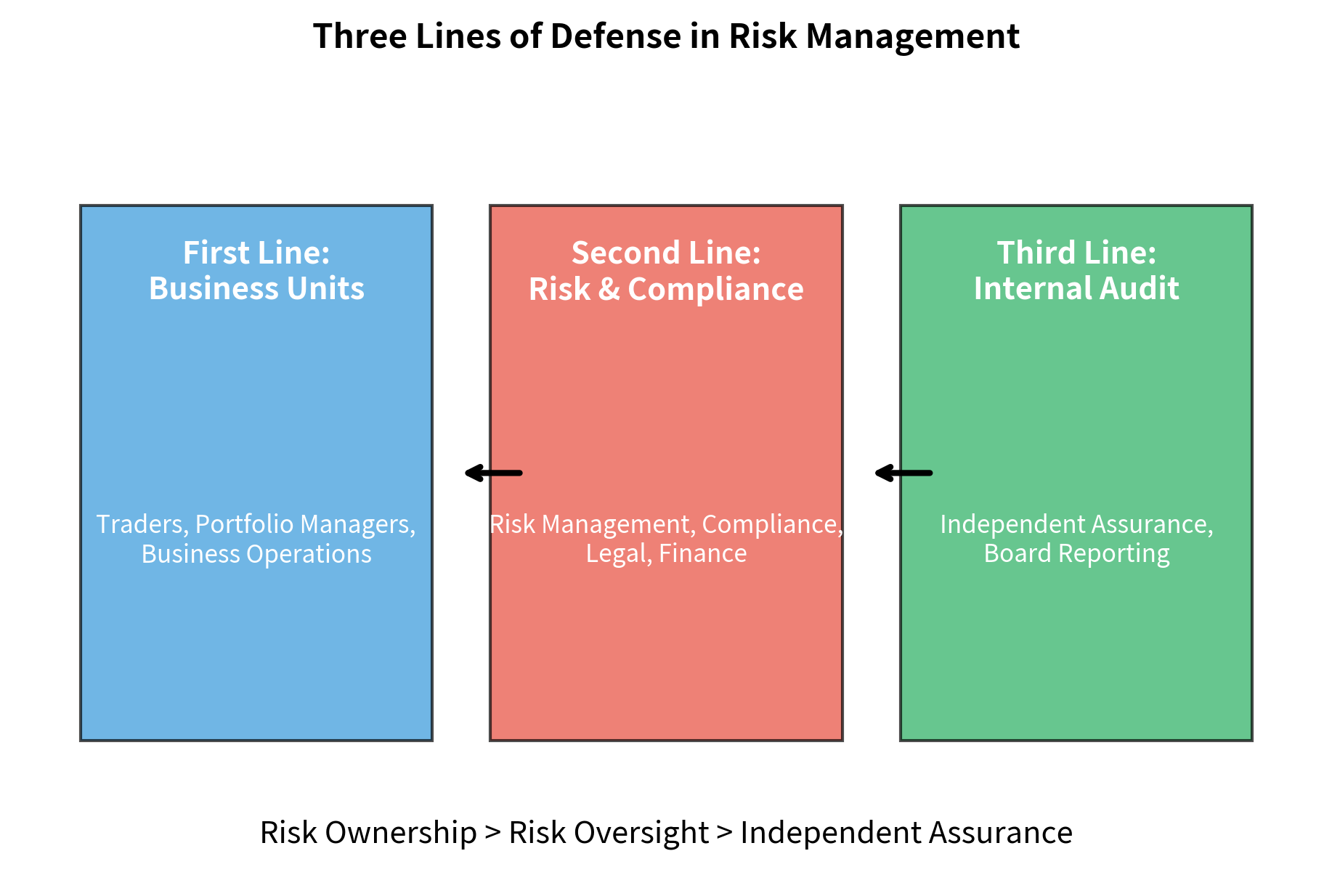
First Line (Business Units):
- Owns and manages risk in daily activities
- Implements controls within their operations
- Responsible for identifying and escalating risks
- Includes traders, portfolio managers, operations staff
Second Line (Risk and Compliance Functions):
- Provides independent oversight and challenge
- Sets risk policies and frameworks
- Monitors risk exposures and limit breaches
- Reports to senior management and board
Third Line (Internal Audit):
- Provides independent assurance on control effectiveness
- Tests that first and second line functions work as designed
- Reports directly to audit committee and board
Risk Limits and Controls
Risk management implements controls through a hierarchy of limits and thresholds:
Position limits restrict the size of individual positions:
- Notional limits (e.g., maximum \$10 million in any single name)
- Concentration limits (e.g., maximum 5% of portfolio in any sector)
- Gross exposure limits (e.g., maximum 200% gross exposure)
Risk metric limits restrict aggregate risk measures:
- VaR limits (e.g., 1-day 99% VaR not to exceed $5 million)
- Stress loss limits (e.g., losses under defined stress scenarios not to exceed $20 million)
- Greeks limits for options books (e.g., delta, gamma, vega bounds)
Loss limits trigger action based on realized losses:
- Stop-loss limits (e.g., mandatory position reduction after 3% daily loss)
- Drawdown limits (e.g., trading halt after 15% monthly drawdown)
- Margin call thresholds
The following Python function assesses risk limit utilization against defined thresholds and generates a status dashboard.
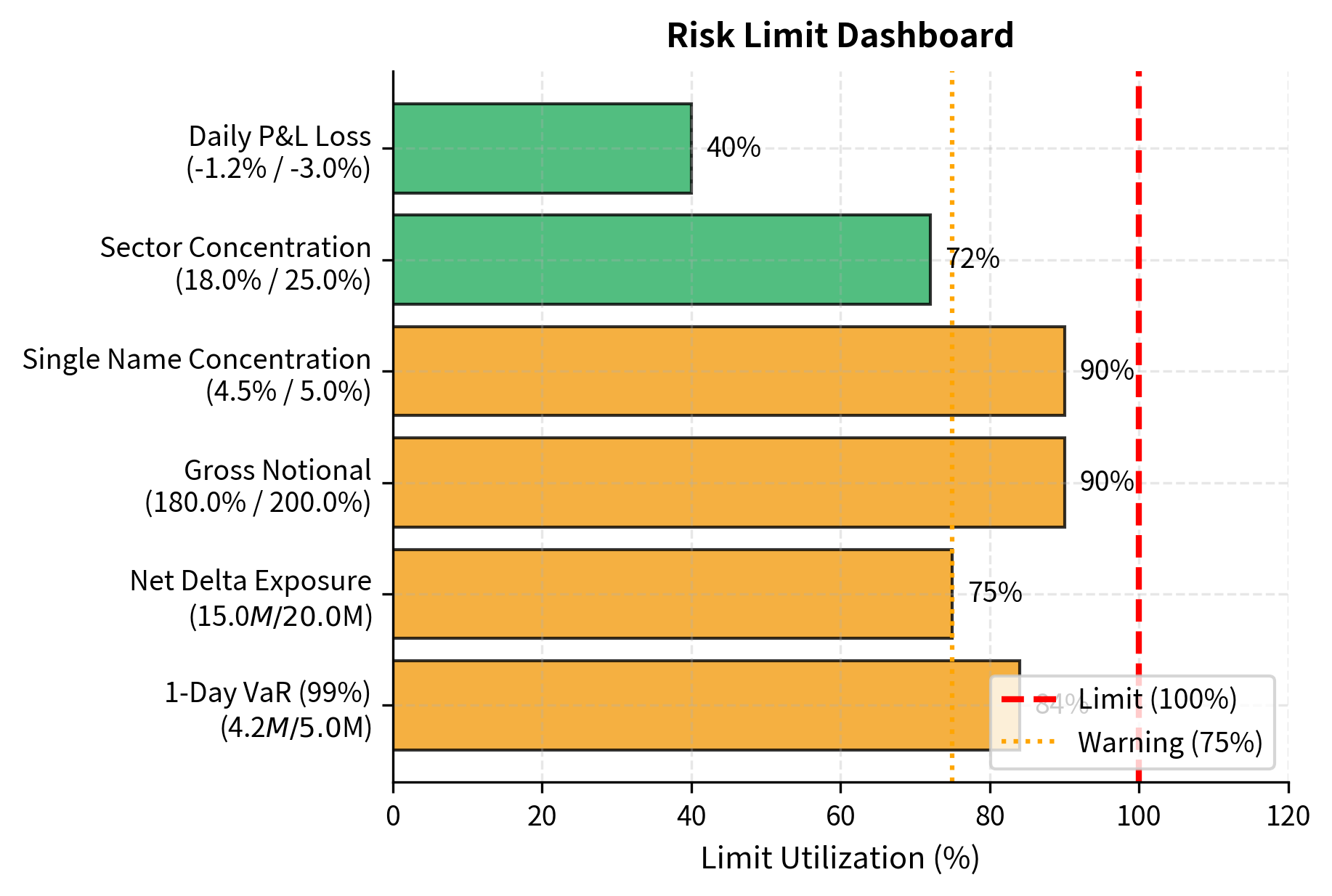
The dashboard highlights that while no hard limits have been breached, several metrics, including VaR and Concentration limits, have triggered warnings (exceeding 75% utilization). This clustering of warnings alerts risk managers to heighten monitoring and potentially reduce exposures before hard limits are violated.
Key Parameters
The risk limit monitoring logic uses the following parameters to translate raw exposures into actionable status indicators:
- current: The current utilization of the risk metric (e.g., VaR amount, gross exposure). This is the actual measured value from the portfolio or trading book.
- limit: The maximum allowable value for the metric. Limits are set by risk committees based on risk appetite, capital constraints, and regulatory requirements.
- warning_pct: The threshold (75%) at which the status shifts from 'OK' to 'WARNING'. This early warning allows risk managers to take preemptive action before hard limits are breached, reducing the likelihood of forced position reductions that might occur at disadvantageous prices.
- utilization: The ratio of current exposure to the limit. Values above 1.0 indicate a breach. This ratio provides a normalized measure that allows comparison across metrics with different units and scales.
Risk Committees and Escalation
Formal governance structures ensure that risk information reaches appropriate decision-makers:
- Risk Committee: Senior management committee that reviews aggregate risk positions, approves limit frameworks, and addresses significant risk issues. Typically meets weekly or monthly.
- ALCO (Asset-Liability Committee): Focuses on balance sheet risks, funding, and liquidity for institutions with significant liability management needs.
- Escalation procedures: Defined processes for reporting limit breaches, significant losses, and emerging risks. Clear accountability for who must be notified and what actions must be taken.
The key principle is that risk decisions should be made at appropriate levels: routine limit management by front-office risk managers, significant issues by senior management, and strategic risk decisions by boards and executive committees.
Interactions Among Risk Types
While we have categorized risks into distinct types, in practice these risks interact and compound each other. Understanding these interactions is essential for comprehensive risk management.
Risk Cascades
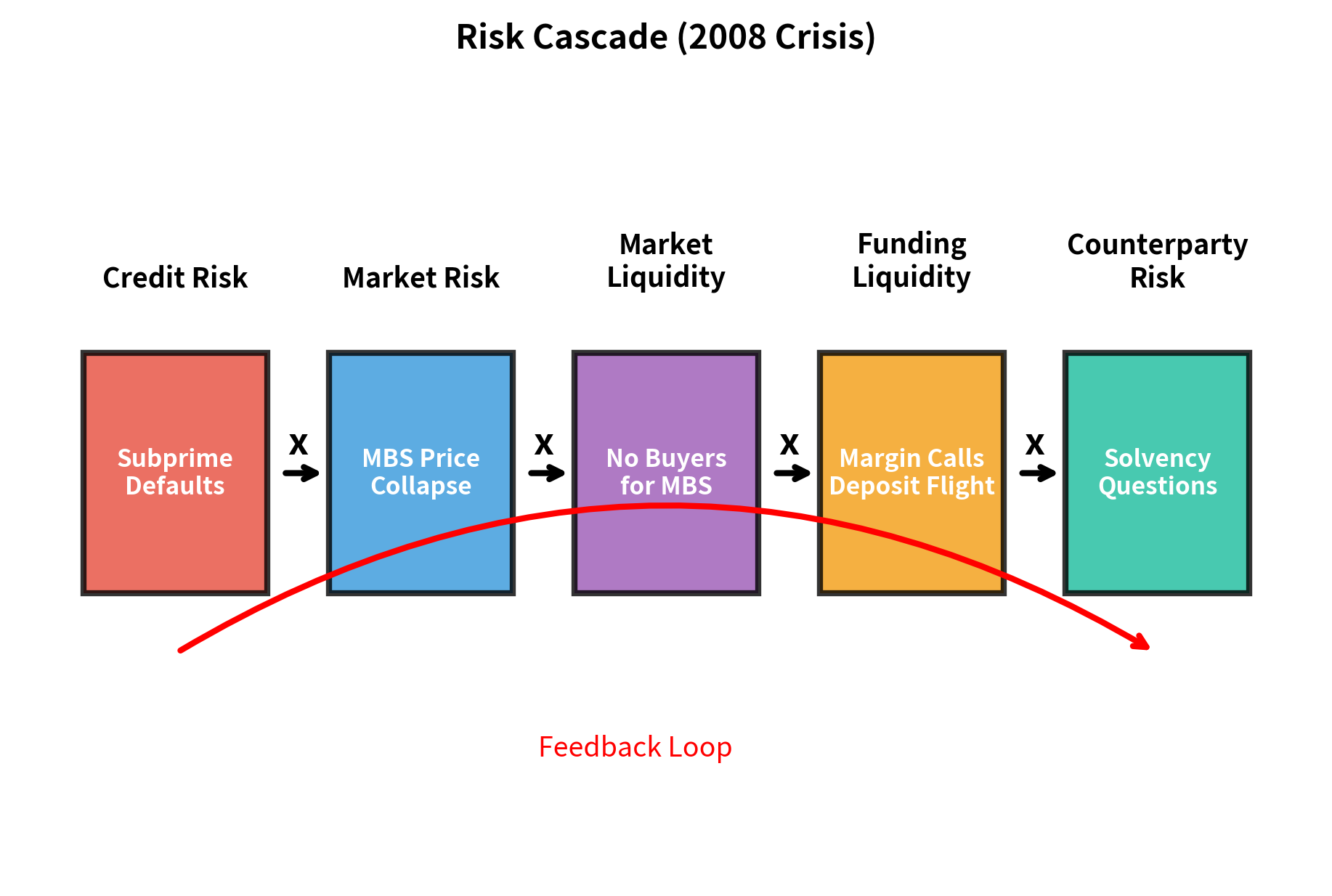
The 2008 financial crisis illustrated how risks can cascade:
- Credit losses on subprime mortgages impaired the value of mortgage-backed securities
- Market risk materialized as MBS prices fell, causing mark-to-market losses
- Liquidity risk emerged as investors fled the MBS market, eliminating secondary market liquidity
- Funding liquidity risk intensified as banks holding MBS faced margin calls and deposit flight
- Counterparty credit risk spiked as questions emerged about institution solvency
- Operational challenges arose from the complexity of structured products whose documentation and servicing hadn't anticipated mass defaults
Each risk type amplified the others, creating a systemic crisis far worse than any single risk in isolation would have caused.
Correlation Breakdown
A particularly dangerous interaction involves the breakdown of diversification during stress events. Correlations between asset classes, which appear low during normal times, spike during crises:
- Emerging market equities and developed market equities become highly correlated during global selloffs
- Credit spreads and equity volatility move together during risk-off episodes
- Commodity prices, usually driven by specific supply-demand factors, become correlated with financial assets during liquidity crises
This means that diversification, the primary tool for managing market risk, becomes less effective precisely when it is most needed. Risk management must account for this through stress testing that assumes elevated correlations.
We can simulate the breakdown of diversification by comparing correlation matrices under normal and crisis conditions. The intuition is straightforward: during normal times, different assets respond to different factors, so their correlations are moderate. During crises, a single dominant factor (often related to liquidity or risk appetite) drives all risky assets simultaneously, causing correlations to converge toward extremes.
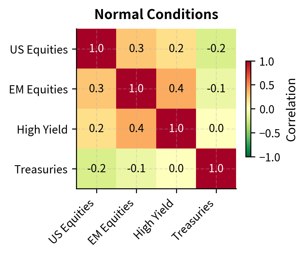
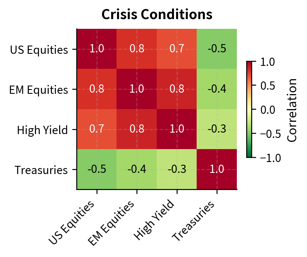
The shift from normal to crisis correlations has profound implications. A portfolio that appeared well-diversified under normal correlations may have much higher risk under crisis correlations. Robust risk management evaluates portfolio risk under both scenarios. Notice in particular how the correlation between US Equities and EM Equities jumps from 0.3 to 0.8, and the correlation between EM Equities and High Yield jumps from 0.4 to 0.85. These asset classes, which provide meaningful diversification during calm periods, move nearly in lockstep during crises.
Key Parameters
The correlation breakdown simulation compares two distinct market regimes:
- normal_corr: A correlation matrix representing standard market conditions with lower cross-asset correlations, supporting diversification. During normal times, different factors drive different asset classes: US equities respond to domestic earnings and Fed policy, emerging markets respond to local conditions and currency movements, high yield responds to credit fundamentals, and Treasuries respond to inflation expectations and flight-to-quality flows.
- crisis_corr: A correlation matrix representing stressed conditions where correlations converge toward 1.0 (or -1.0), reducing the benefit of diversification. During crises, a single dominant factor, often related to global risk appetite or liquidity conditions, drives all risky assets simultaneously downward while safe assets benefit from flight-to-quality flows.
Limitations and Practical Considerations
Risk management faces inherent limitations that practitioners must acknowledge and address through judgment, conservatism, and humility.
The most fundamental limitation is that risk models are backward-looking while risks materialize in the future. Models calibrated on historical data assume that the future resembles the past. This assumption fails precisely during the market dislocations that matter most. The 2008 crisis exposed models that had been calibrated on decades of data without a nationwide housing price decline; those models systematically underestimated the risk of correlated mortgage defaults because such an event had not occurred in the calibration window.
This limitation cannot be fully overcome through better models. The future is genuinely uncertain, and some events ("black swans") lie outside the realm of historical experience and statistical estimation. Risk management must therefore combine quantitative tools with scenario analysis, stress testing, and expert judgment to address risks that models cannot capture.
A second limitation is the trade-off between risk management and business goals. Every limit that prevents excessive risk-taking also potentially constrains profitable opportunities. Risk management must balance safety with the firm's need to generate returns. This tension is healthy; it forces explicit discussion of risk appetite and ensures that risk-taking is intentional. However, it creates organizational pressures that risk managers must navigate carefully.
Finally, risk management can create a false sense of security. Sophisticated models and elaborate governance structures may lead to overconfidence, encouraging risk-taking that wouldn't occur if participants acknowledged how much they don't know. The history of financial crises is littered with institutions whose risk management was considered state-of-the-art until it wasn't. Effective risk management requires intellectual humility: the recognition that our models are approximations, our data is limited, and the future will surprise us in ways we cannot anticipate.
Summary
This chapter has provided a comprehensive overview of financial risks and the frameworks used to manage them. The key concepts we have covered form the foundation for the detailed quantitative techniques in the chapters that follow.
Risk categories provide a taxonomy for thinking about financial threats:
- Market risk arises from adverse movements in prices, rates, and volatilities
- Credit risk arises from counterparty failure to meet obligations
- Liquidity risk arises from inability to transact or meet obligations without unacceptable costs
- Operational risk arises from failures in processes, people, systems, or external events
- Model risk arises from flawed or misapplied quantitative models
Risk management objectives extend beyond simple loss avoidance:
- Protecting capital and ensuring survival through tail events
- Meeting regulatory requirements
- Optimizing risk-adjusted returns by allocating risk to compensated exposures
Regulatory frameworks, particularly Basel III, shape institutional behavior through:
- Risk-weighted capital requirements
- Liquidity coverage and stable funding ratios
- Leverage limits
- Stress testing requirements
Organizational structures translate these objectives into practice through:
- The three lines of defense: business ownership, independent oversight, and internal audit
- Hierarchical risk limits covering positions, risk metrics, and losses
- Governance committees and escalation procedures
Risk interactions mean that categories cannot be managed in isolation; cascading failures and correlation breakdown during crises amplify individual risks into systemic events.
In the next chapter, we will dive deep into the quantitative measurement of market risk, developing Value at Risk and its extensions as tools for estimating potential losses. We will then proceed through credit risk modeling, counterparty risk, and liquidity risk, building a comprehensive toolkit for risk measurement and management.
Quiz
Ready to test your understanding? Take this quick quiz to reinforce what you've learned about financial risks and regulatory frameworks.

Comments