Advanced Portfolio Construction: Black-Litterman & Risk Parity

Mean-variance optimization, introduced by Markowitz and covered in our earlier discussion of Modern Portfolio Theory, provides an elegant theoretical framework for portfolio construction. The approach offers mathematical precision: given expected returns and a covariance matrix, we can identify portfolios that deliver the maximum return for any given level of risk. However, we quickly discovered that applying MVO directly to real-world portfolios often produces disappointing results. The optimized portfolios tend to concentrate heavily in a small number of assets, exhibit extreme long and short positions, and suffer from poor out-of-sample performance. These pathologies arise not from flaws in the theory itself, but from the sensitivity of the optimization to estimation errors in expected returns and covariances. When we treat uncertain estimates as if they were known truths, the optimizer exploits our estimation errors just as eagerly as it exploits genuine opportunities.

This chapter addresses these challenges through four complementary approaches. We begin with the Black-Litterman model, which provides a principled way to combine market equilibrium returns with your views. Rather than estimating expected returns from scratch, Black-Litterman starts from a stable reference point and adjusts it based on your beliefs. We then examine robust optimization techniques that explicitly account for parameter uncertainty by designing portfolios that perform well across a range of possible parameter values. Next, we explore how to incorporate practical constraints such as position limits, turnover restrictions, and sector exposures, transforming theoretical optimization into implementable portfolio management. Finally, we introduce risk parity, an alternative paradigm that constructs portfolios based on risk contributions rather than expected returns, offering a fundamentally different perspective on diversification.

These techniques represent the evolution from academic portfolio theory to institutional practice. Understanding them is essential for you to build portfolios that perform well not just in theory, but in the messy reality of financial markets where parameters are uncertain, constraints are numerous, and implementation costs are real.

Before diving into solutions, we must first understand why traditional MVO fails in practice. The problem is not conceptual but statistical: we are asking the optimizer to work with inputs that we cannot measure precisely. Recall from Part IV, Chapter 1 that mean-variance optimization finds the portfolio weights $\mathbf{w}$ that minimize portfolio variance for a given target return:

where:

• $\mathbf{w}$: vector of portfolio weights
• $\boldsymbol{\Sigma}$: asset covariance matrix
• $\boldsymbol{\mu}$: vector of expected asset returns
• $\mu_p$: target portfolio return
• $\mathbf{1}$: vector of ones (sum of weights constraint)

The mathematical elegance of this formulation masks a fundamental challenge: every input to this optimization must be estimated from historical data, and even small estimation errors can produce dramatically different optimal portfolios. To understand why, consider what the optimizer is doing. It searches for the portfolio that achieves the target return with minimum variance, which means it naturally gravitates toward assets that appear to have high returns and low volatilities, while avoiding assets that seem risky or poorly performing. The problem is that "appear to have" and "seem" are doing a lot of work in that sentence. An asset that happened to perform well in our historical sample might have been lucky rather than fundamentally superior. An asset with low measured volatility might simply have experienced a calm period. The optimizer cannot distinguish genuine signal from noise, so it treats every fluctuation in our estimates as real information to be exploited.

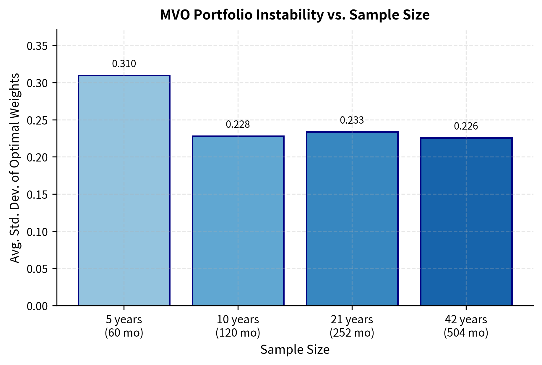
The results reveal a troubling sensitivity: even with several years of data, the "optimal" weights fluctuate dramatically depending on which particular sample we observe. With five years of monthly data (60 observations), the standard deviation of optimal weights across simulations is substantial. Even with over 40 years of data (504 observations), the instability remains problematic. This instability arises because MVO treats the estimated parameters as if they were known with certainty, when in fact they are noisy estimates of unknown true values. The optimizer has no mechanism to express doubt or hedge against the possibility that its inputs are wrong.

The Black-Litterman model, developed by Fischer Black and Robert Litterman at Goldman Sachs in 1990, addresses the estimation problem by starting from a stable reference point: the market equilibrium. The key insight is that if we have no special information about expected returns, we should assume the market is in equilibrium, meaning current prices are fair and expected returns reflect risk. Rather than estimating expected returns from historical data, which is notoriously unreliable, Black-Litterman reverse-engineers the expected returns implied by market capitalization weights, then adjusts these based on your views. This approach sidesteps the return estimation problem while providing a systematic framework for incorporating investment insights.

The first insight underpinning the Black-Litterman model is that if markets are in equilibrium and investors hold the market portfolio, we can infer the expected returns that would make the market portfolio optimal. This is reverse optimization: rather than using expected returns to find optimal weights, we use the observed weights (market capitalizations) to deduce what expected returns market participants must believe. The logic is compelling: if millions of investors, collectively representing the market, have chosen to hold assets in certain proportions, then the expected returns implied by those proportions represent a kind of consensus expectation.

We start with the unconstrained mean-variance utility function with risk aversion $\delta$. You seek to maximize utility, defined as expected return minus a penalty for variance. The penalty captures your discomfort with uncertainty: higher variance means more potential for adverse outcomes, and you demand compensation for bearing that risk.

where:

• $U$: investor utility
• $\mathbf{w}$: vector of portfolio weights
• $\boldsymbol{\Pi}$: vector of expected excess returns
• $\delta$: risk aversion coefficient
• $\boldsymbol{\Sigma}$: covariance matrix of asset returns

The utility function captures a fundamental tradeoff. The first term, $\mathbf{w}^T \boldsymbol{\Pi}$, represents the expected return of the portfolio: higher returns increase utility. The second term, $\frac{\delta}{2} \mathbf{w}^T \boldsymbol{\Sigma} \mathbf{w}$, represents a penalty for portfolio variance: higher variance decreases utility. The parameter $\delta$ determines how severely you penalize variance. If you are highly risk-averse (large $\delta$), you will sacrifice substantial expected return to reduce variance, while if you are more risk-tolerant (small $\delta$), you will accept higher variance in pursuit of higher returns.

To find the implied equilibrium returns, we solve for the return vector that makes the market portfolio optimal. Setting the gradient of the utility function to zero gives us the first-order condition for optimality:

where:

• $\boldsymbol{\Pi}$: vector of implied equilibrium excess returns
• $\delta$: risk aversion coefficient of the market representative investor
• $\boldsymbol{\Sigma}$: covariance matrix of asset returns
• $\mathbf{w}$: vector of portfolio weights
• $\mathbf{w}_{mkt}$: vector of market capitalization weights

This derivation reveals a powerful insight: given the covariance matrix and market weights, we can back out the expected returns that rational investors must collectively believe. The formula $\boldsymbol{\Pi} = \delta \boldsymbol{\Sigma} \mathbf{w}_{mkt}$ tells us that implied returns depend on both the asset's own risk contribution (through the covariance matrix) and its market weight. Assets that receive large allocations in the market portfolio must offer attractive risk-adjusted returns, or investors would not hold them. Conversely, assets with small market weights must offer less attractive returns, or investors would demand more of them.

These implied returns have a crucial advantage over historical estimates: by construction, they produce the market portfolio as the optimal solution. If we were to run mean-variance optimization using these returns, we would recover exactly the market capitalization weights. This makes them a natural, stable starting point. They represent a neutral prior that says, "In the absence of any special views, we believe current market prices are fair." From this baseline, we can then incorporate our own investment insights to tilt the portfolio away from the market.

The second component of Black-Litterman is a framework for expressing and incorporating your views. Views are expressed as linear combinations of asset returns, providing flexibility to capture both absolute predictions ("Asset X will return Y%") and relative predictions ("Asset X will outperform Asset Z by Y%"). This flexibility is essential because many investment insights are naturally expressed in relative terms. We might believe technology will outperform financials without having strong convictions about either sector's absolute return.

The mathematical representation of views takes the following form:

where:

• $\mathbf{P}$: $k \times n$ matrix specifying $k$ views on $n$ assets
• $\boldsymbol{\mu}$: vector of expected asset returns
• $\mathbf{Q}$: $k \times 1$ vector of view returns
• $\boldsymbol{\epsilon}$: error term capturing uncertainty in the views
• $\boldsymbol{\Omega}$: covariance matrix of view errors

Each row of $\mathbf{P}$ corresponds to one view, and the entries in that row indicate which assets are involved and with what weights. For an absolute view on a single asset, the row contains a 1 in that asset's column and zeros elsewhere. For a relative view comparing two assets, the row contains a 1 for the asset expected to outperform and a -1 for the asset expected to underperform. More complex views involving multiple assets can be expressed through appropriate combinations of positive and negative weights.

The vector $\mathbf{Q}$ specifies the expected returns associated with each view. For an absolute view, this is simply the predicted return. For a relative view, it is the expected outperformance. The error term $\boldsymbol{\epsilon}$ acknowledges that views are uncertain: we might believe Asset B will outperform Asset A by 3%, but we recognize this prediction could be wrong. The covariance matrix $\boldsymbol{\Omega}$ captures how uncertain we are about each view, with larger values indicating less confidence.

Black-Litterman combines the equilibrium prior with your views using Bayesian updating, a principled statistical framework for combining prior beliefs with new information. The approach weights different sources of information according to their precision: strong views with high confidence will move the posterior returns substantially, while weak views with low confidence will have little effect. Similarly, if the equilibrium prior is considered very precise (small $\tau$), views will have less impact, but if the prior is considered uncertain (larger $\tau$), views will be more influential.

The posterior expected returns are given by:

where:

• $\boldsymbol{\mu}_{BL}$: posterior expected return vector
• $\tau$: scalar scaling factor for the uncertainty of the prior
• $\boldsymbol{\Sigma}$: covariance matrix of asset returns
• $\mathbf{P}$: matrix identifying the assets involved in the views
• $\boldsymbol{\Omega}$: diagonal covariance matrix of view error terms
• $\boldsymbol{\Pi}$: vector of implied equilibrium returns
• $\mathbf{Q}$: vector of expected returns for the views

While this formula may appear complex at first glance, its structure becomes clear when we understand it as a precision-weighted average of two information sources. In Bayesian statistics, precision is the inverse of variance and represents how confident we are about an estimate. Higher precision means greater confidence.

The formula decomposes into these interpretable components:

• $(\tau \boldsymbol{\Sigma})^{-1}$: the precision (inverse covariance) of the market equilibrium prior. Smaller $\tau$ means higher precision, making the prior more influential.
• $\mathbf{P}^T \boldsymbol{\Omega}^{-1} \mathbf{P}$: the precision of your views projected onto the asset space. Smaller $\boldsymbol{\Omega}$ means higher precision, making the views more influential.
• The first bracketed term, $[(\tau \boldsymbol{\Sigma})^{-1} + \mathbf{P}^T \boldsymbol{\Omega}^{-1} \mathbf{P}]^{-1}$, is the inverse of total precision, combining information from both sources.
• The second bracketed term sums the precision-weighted returns from the prior ($(\tau \boldsymbol{\Sigma})^{-1} \boldsymbol{\Pi}$) and the views ($\mathbf{P}^T \boldsymbol{\Omega}^{-1} \mathbf{Q}$).

This structure essentially pulls the posterior means away from the equilibrium returns toward the views, with the degree of pull depending on the relative confidence in each source. The parameter $\tau$ (typically ranging from 0.01 to 0.10) controls how much weight is given to the prior relative to the views. A smaller $\tau$ makes the prior more precise and harder to move, while a larger $\tau$ makes the prior less precise and more susceptible to being influenced by views.

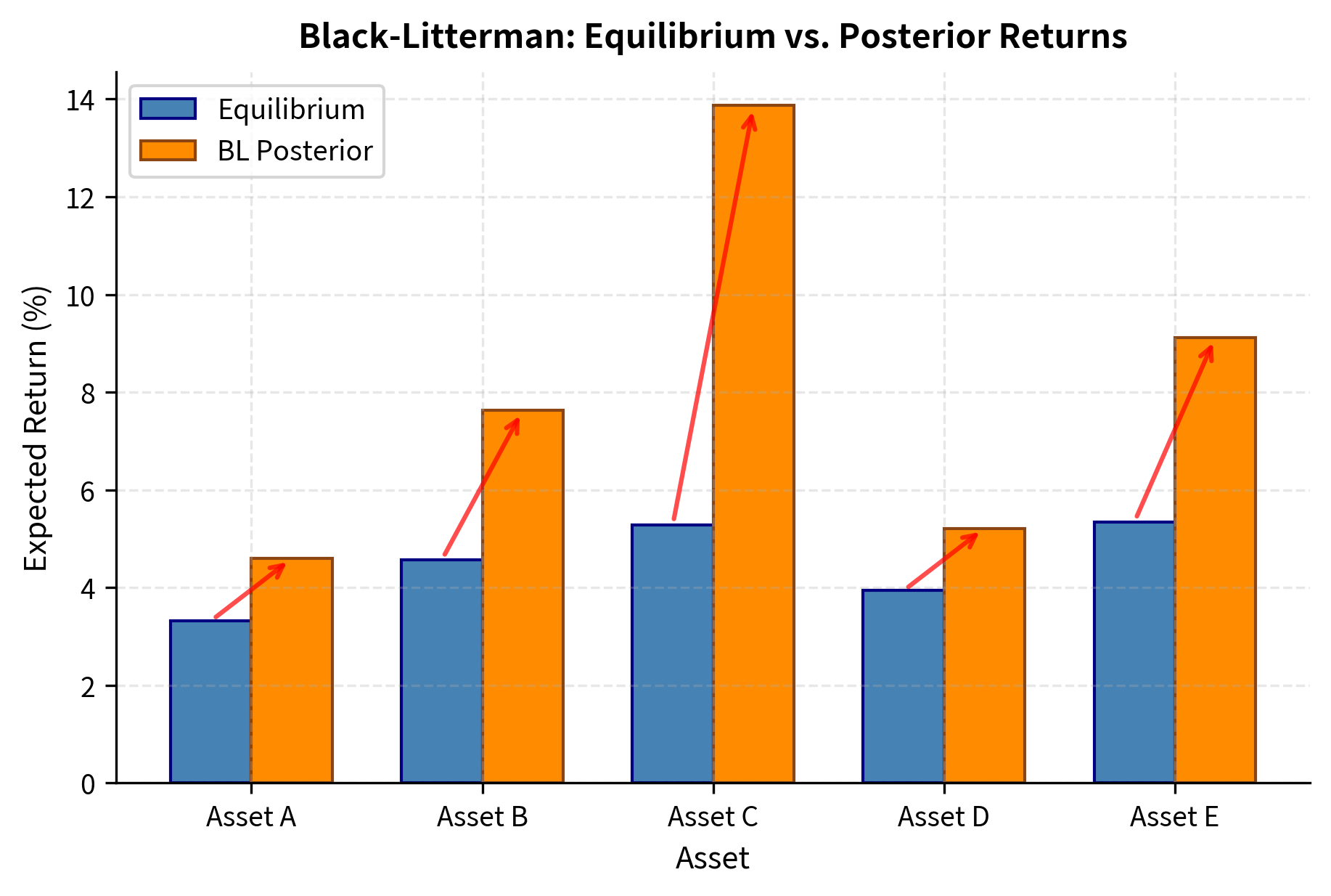
Notice how the posterior returns reflect our views in an intuitive way: Asset C's expected return increased toward 15%, and Asset B's return increased relative to Asset A. But the model also captures something subtler: the other assets' returns shifted slightly due to their correlations with the view assets. When we become more bullish on Asset C, we implicitly become somewhat more bullish on assets correlated with C. This propagation of views through the correlation structure is one of the elegant features of Black-Litterman.

With the posterior expected returns in hand, we can now perform mean-variance optimization with stable, economically sensible inputs. The resulting portfolio will tilt toward our views while maintaining reasonable diversification, avoiding the extreme positions that plague traditional MVO.

The Black-Litterman portfolio tilts toward assets favored by our views (C and B) while maintaining reasonable diversification across all five assets. This is markedly different from what traditional MVO would produce: the equilibrium anchor prevents extreme positions, while the view-blending mechanism systematically incorporates our investment insights. Without views, the equilibrium portfolio would closely resemble the market portfolio, providing a stable default that requires positive conviction to deviate from.

While Black-Litterman addresses the expected return estimation problem through a clever change in starting point, robust optimization takes a fundamentally different approach: explicitly acknowledging that we do not know the true parameters and designing portfolios that perform well across a range of possible values. Rather than pretending we have precise estimates, robust optimization admits uncertainty and hedges against it.

The core idea of robust optimization is to represent parameter uncertainty through uncertainty sets. Rather than assuming we know the exact expected return vector $\boldsymbol{\mu}$, we specify a set $\mathcal{U}$ of possible values that $\boldsymbol{\mu}$ might take. The robust portfolio then maximizes performance in the worst-case scenario within this set:

where:

• $\mathbf{w}$: portfolio weight vector
• $\mathcal{U}$: set of possible expected return vectors
• $\boldsymbol{\mu}$: expected return vector
• $\delta$: risk aversion parameter
• $\boldsymbol{\Sigma}$: covariance matrix (assumed known here)

This formulation reflects a pessimistic but prudent worldview: nature will choose the returns within our uncertainty set that are worst for our chosen portfolio, and we should pick the portfolio that performs best even under this adversarial scenario. The objective function balances two competing goals:

• $\min_{\boldsymbol{\mu} \in \mathcal{U}} \mathbf{w}^T \boldsymbol{\mu}$: finds the worst-case expected return within the uncertainty set for a given allocation. This term captures the downside risk from parameter uncertainty.
• $\frac{\delta}{2} \mathbf{w}^T \boldsymbol{\Sigma} \mathbf{w}$: penalizes portfolio variance based on the risk aversion parameter $\delta$. This term captures the traditional risk-return tradeoff.

The most common uncertainty set in practice is ellipsoidal, based on the statistical confidence region for estimated means. If we have estimated our mean returns from a sample, statistical theory tells us that the true mean lies within an ellipsoid centered at our estimate with high probability:

where:

• $\mathcal{U}$: uncertainty set for the expected returns
• $\boldsymbol{\mu}$: true (unknown) expected return vector
• $\hat{\boldsymbol{\mu}}$: estimated mean vector from data
• $\mathbf{S}$: estimation error covariance matrix
• $\kappa$: parameter controlling the size of the uncertainty set (confidence level)

The shape of this ellipsoid reflects the correlation structure of estimation errors. If two assets' returns are highly correlated, our estimates of their means will also be correlated, and the ellipsoid will be elongated along the direction where both returns move together. The parameter $\kappa$ controls the size of the uncertainty set, with larger values corresponding to higher confidence levels but also more conservative portfolios.

With $\kappa=0$, we recover the standard MVO weights, which are often concentrated in assets that happen to have the highest estimated returns. As $\kappa$ increases, the optimization accounts for greater uncertainty, leading to more conservative and diversified portfolios. The robust optimizer recognizes that concentrated bets on high-return assets are risky if those high returns turn out to be estimation errors.

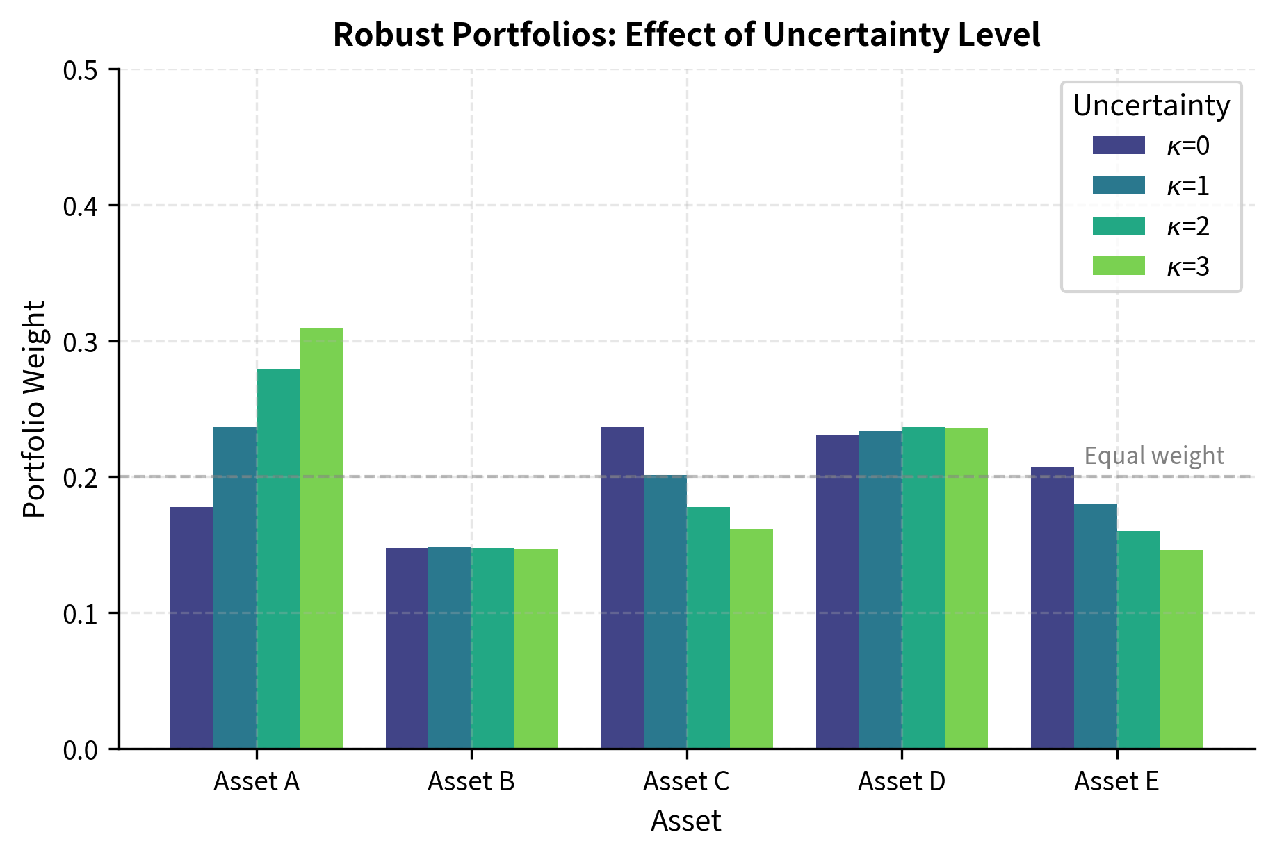
As the uncertainty level $\kappa$ increases, the robust portfolio becomes progressively more conservative and diversified. With $\kappa = 0$, we recover standard MVO, which assumes our estimates are perfectly accurate. But as uncertainty grows, the optimizer hedges against the possibility that its estimates are wrong by spreading risk across more assets. This behavior is precisely what we want: when we are uncertain, we should not make large bets.

An alternative approach to robust optimization is resampled efficiency, proposed by Richard Michaud in the 1990s. Rather than specifying an explicit uncertainty set and solving a worst-case problem, resampling uses Monte Carlo simulation to capture the range of possible optimal portfolios consistent with our estimation uncertainty. The approach is intuitive and requires no special optimization software.

The resampling procedure works as follows: First, generate many bootstrap samples from the return distribution by sampling with replacement from historical returns. Second, compute the optimal portfolio for each bootstrap sample using standard mean-variance optimization. Third, average the resulting weights across all samples to obtain the resampled efficient portfolio.

The averaging step is crucial. Each bootstrap sample produces a slightly different "optimal" portfolio, reflecting the fact that our estimates fluctuate with the data. Some samples will favor Asset A, others will favor Asset B. By averaging across samples, we obtain a portfolio that is robust to the particular quirks of any single sample. Assets that are consistently favored across samples will receive high average weights, while assets that are favored only in some samples will receive lower average weights.

The resampled portfolio is typically more diversified than the single-sample MVO portfolio. The standard deviation column reveals which assets have stable optimal weights across bootstrap samples (low standard deviation) versus which assets have volatile optimal weights (high standard deviation). This information itself is valuable: assets with high weight volatility are those where our estimate is most uncertain, and we should perhaps be cautious about large positions in them.

Another powerful technique for improving portfolio stability is shrinkage estimation of the covariance matrix. The sample covariance matrix, computed directly from historical returns, is an unbiased estimator of the true covariance matrix, meaning it is correct on average. However, it is also a high-variance estimator, meaning any particular sample can produce estimates that are far from the truth. This is particularly problematic when the number of assets is large relative to the number of time periods, a common situation in portfolio management.

Shrinkage reduces variance by pulling the estimate toward a structured target. The intuition is that while we do not know the true covariance matrix, we do know some things about its general structure. For example, we might believe that correlations are positive on average, or that volatilities do not differ too dramatically across assets. By shrinking toward a target that embodies these beliefs, we trade off some bias for a reduction in variance, often improving overall estimation accuracy.

The Ledoit-Wolf estimator, one of the most popular shrinkage approaches, shrinks the sample covariance toward a scaled identity matrix:

where:

• $\hat{\boldsymbol{\Sigma}}_{\text{shrink}}$: the shrunk covariance matrix estimator
• $\alpha$: shrinkage intensity constant between 0 and 1
• $\mathbf{S}$: sample covariance matrix
• $\mathbf{I}$: identity matrix
• $n$: number of assets (dimension of the covariance matrix)
• $\text{tr}(\cdot)$: trace operator (sum of diagonal elements)

The shrinkage intensity $\alpha$ is typically estimated from the data using a formula that balances bias and variance optimally. A value of $\alpha = 0$ gives the raw sample covariance, while $\alpha = 1$ gives a diagonal matrix with equal variances (the scaled identity). The optimal $\alpha$ depends on the ratio of assets to observations and the dispersion of the true eigenvalues.

Shrinkage pulls the covariance estimate toward a structured target (the identity matrix), reducing the impact of noise in the off-diagonal elements. This results in a portfolio that is less concentrated than the one based on the raw sample covariance, as the extreme correlations in the sample data are dampened. Pairs of assets that appeared highly correlated in the sample are assumed to have somewhat lower true correlation, and pairs that appeared uncorrelated are assumed to have some positive correlation. This conservative approach often leads to better out-of-sample performance.

Real-world portfolios face numerous constraints beyond the basic budget constraint that weights must sum to one. Incorporating these constraints transforms portfolio optimization from a theoretical exercise into a practical tool that produces implementable recommendations. A portfolio that is "optimal" in theory but violates regulatory limits or exceeds trading capacity is useless in practice.

You typically face several categories of constraints, each arising from different practical considerations:

• Position limits: Minimum and maximum weights for individual assets. Regulatory requirements, risk limits, or liquidity concerns often mandate these bounds. For example, a mutual fund might be prohibited from holding more than 10% in any single security, or a pension fund might require minimum allocations to certain asset classes.
• Sector/industry constraints: Maximum exposure to any single sector or minimum allocation to certain sectors (e.g., ESG mandates). These constraints ensure diversification across different parts of the economy and can implement policy objectives like promoting sustainable investment.
• Turnover constraints: Limits on how much the portfolio can change from one period to the next, driven by transaction costs or tax considerations. Frequent rebalancing incurs trading costs and may trigger taxable events, so many investors limit how aggressively they adjust positions.
• Factor exposure constraints: Limits on exposure to risk factors like beta, size, or value. These constraints allow you to control your portfolio's sensitivity to systematic risk drivers, maintaining a desired risk profile regardless of individual security selection.
• Cardinality constraints: Limits on the number of assets in the portfolio (often driven by monitoring costs). Managing a portfolio of 500 securities requires more resources than managing 50, so some investors cap the number of holdings.

Let us build a constrained portfolio optimizer that handles position limits, sector constraints, and turnover simultaneously. The key insight is that most constraints can be expressed as linear or simple nonlinear functions of the weights, allowing standard optimization algorithms to find solutions efficiently.

The constrained optimization respects all limits: no asset exceeds 35% weight, sector exposures are capped, and turnover is limited to 15%. While these constraints reduce the theoretical utility compared to an unconstrained optimum, they produce a portfolio that is actually implementable. The gap between the constrained and unconstrained solutions represents the "cost" of being practical, but this cost is usually worth paying for a portfolio that can actually be traded.

When rebalancing a portfolio, transaction costs can significantly impact returns. Every trade incurs costs from bid-ask spreads, market impact, and commissions. For large institutional portfolios, market impact alone can represent tens of basis points per trade. We can incorporate estimated costs directly into the optimization, finding portfolios that balance the benefits of rebalancing against the costs of trading.

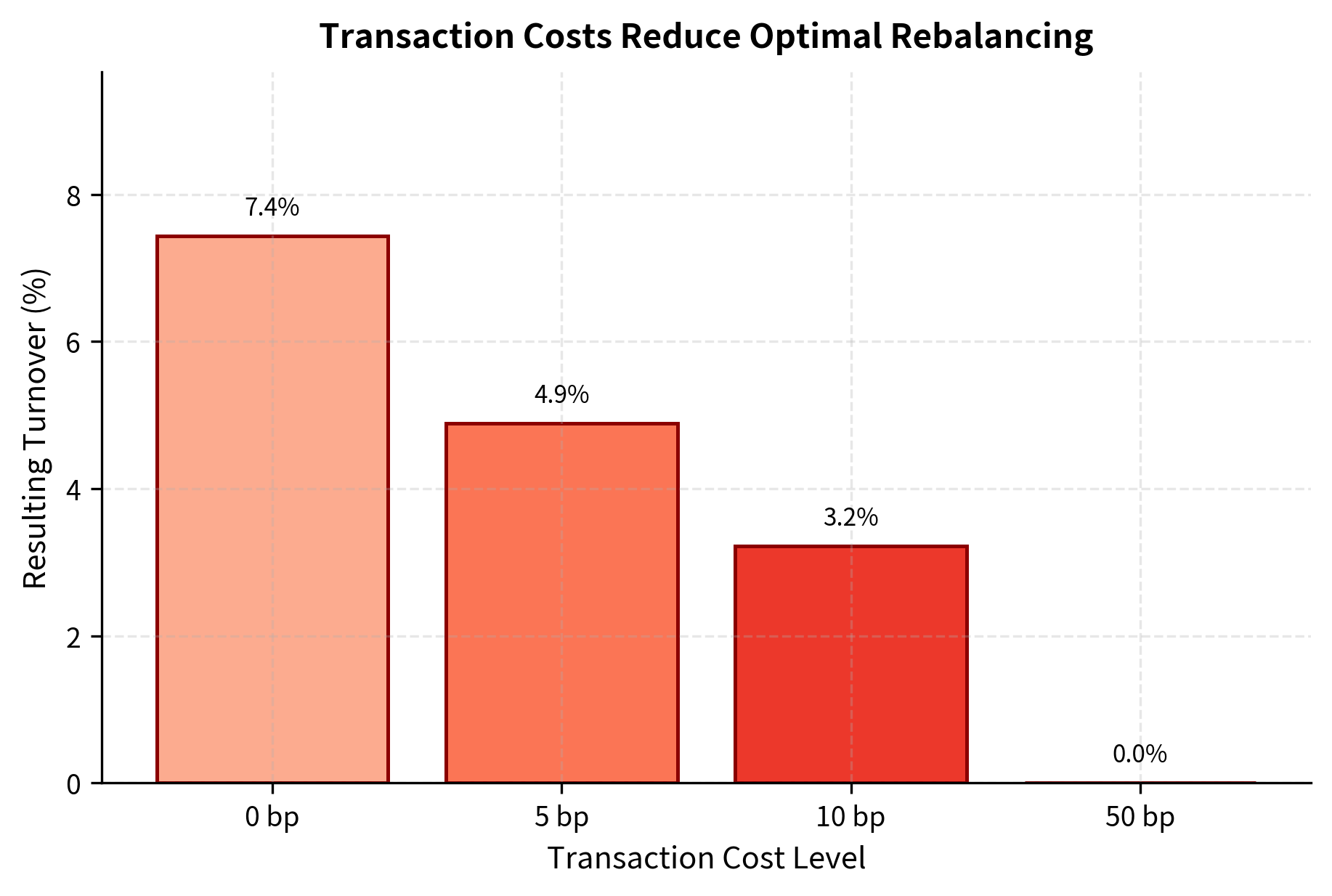
As transaction costs increase, the optimal rebalancing becomes less aggressive. With zero transaction costs, the optimizer freely adjusts weights to chase the best risk-adjusted returns. But at higher cost levels, the optimizer avoids small adjustments where the marginal benefit in risk-adjusted return does not justify the trading expense. This leads to weights closer to the previous portfolio, a phenomenon sometimes called "no-trade regions." The width of these regions depends on the transaction cost level: higher costs mean wider regions and less frequent rebalancing.

Risk parity represents a fundamentally different approach to portfolio construction. Rather than optimizing expected return per unit of risk, risk parity allocates capital so that each asset contributes equally to total portfolio risk. This approach gained prominence after the 2008 financial crisis, when traditional 60/40 stock-bond portfolios suffered large losses due to their concentration of risk in equities. Many investors holding 60% stocks and 40% bonds believed they were diversified, only to discover that over 90% of their portfolio risk came from the equity allocation.

To understand risk parity, we first need to define precisely what we mean by an asset's contribution to portfolio risk. Intuitively, we want to answer the question: if we slightly increase our position in Asset X, how much will our portfolio volatility change? This marginal contribution to risk, combined with the current position size, tells us how much each asset contributes to the total.

The total portfolio volatility can be decomposed into contributions from each asset:

where:

• $\sigma_p$: total portfolio volatility (standard deviation)
• $n$: number of assets
• $w_i$: weight of asset $i$
• $RC_i$: risk contribution of asset $i$

This decomposition follows from Euler's theorem for homogeneous functions: portfolio volatility is homogeneous of degree one in the weights, meaning if we scale all weights by a factor $k$, volatility also scales by $k$. Euler's theorem then guarantees that volatility can be exactly decomposed into the sum of each weight times its marginal contribution.

The marginal contribution to risk (MCR) for asset $i$ is derived from the portfolio volatility derivative using the chain rule:

where:

• $\sigma_p$: portfolio volatility
• $\mathbf{w}$: vector of portfolio weights
• $\boldsymbol{\Sigma}$: covariance matrix of asset returns

This formula has an intuitive interpretation. The term $\boldsymbol{\Sigma} \mathbf{w}$ is a vector whose $i$-th element represents the covariance between asset $i$ and the overall portfolio. An asset's marginal contribution to risk depends not just on its own volatility, but on how it comoves with the portfolio as a whole. An asset with high own volatility but negative correlation with other holdings might actually reduce portfolio risk at the margin.

For a single asset $i$, the MCR is the $i$-th element:

where:

• $MCR_i$: marginal contribution to risk of asset $i$
• $\sigma_p$: portfolio volatility
• $\boldsymbol{\Sigma}$: covariance matrix of asset returns
• $\mathbf{w}$: vector of portfolio weights
• $(\boldsymbol{\Sigma} \mathbf{w})_i$: the $i$-th element of the vector product $\boldsymbol{\Sigma} \mathbf{w}$

The total risk contribution (RC) for asset $i$ combines the position size with the marginal contribution:

where:

• $RC_i$: total risk contribution of asset $i$
• $w_i$: weight of asset $i$
• $MCR_i$: marginal contribution to risk of asset $i$
• $\boldsymbol{\Sigma}$: covariance matrix of asset returns
• $\mathbf{w}$: vector of portfolio weights
• $(\boldsymbol{\Sigma} \mathbf{w})_i$: the $i$-th element of the vector product $\boldsymbol{\Sigma} \mathbf{w}$
• $\sigma_p$: portfolio volatility

By construction, the risk contributions sum to total portfolio volatility: $\sum_{i=1}^{n} RC_i = \sigma_p$. This additive decomposition allows us to express what fraction of portfolio risk comes from each asset, enabling meaningful comparisons across holdings.

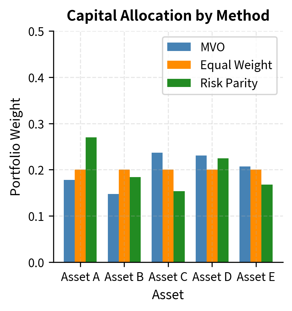
Even with equal capital weights, the risk contributions are far from equal. Higher-volatility assets contribute disproportionately to portfolio risk. Asset C, with 25% volatility, contributes roughly 25% of portfolio risk despite having only 20% of capital. Meanwhile, Asset A, with 15% volatility, contributes only about 15% of risk. This mismatch between capital allocation and risk allocation is precisely what risk parity seeks to address.

A risk parity portfolio equalizes risk contributions across all assets. Rather than asking 'how should you allocate your capital?', risk parity asks 'how should you allocate your risk budget?' The answer is to find weights such that:

where:

• $RC_i$: risk contribution of asset $i$
• $RC_j$: risk contribution of asset $j$

or equivalently, expressed in terms of weights and marginal contributions:

where:

• $w_i, w_j$: weights of assets $i$ and $j$
• $(\boldsymbol{\Sigma} \mathbf{w})_k$: the $k$-th element of the covariance-weight product (proportional to marginal risk)

This is a nonlinear system of equations because the marginal contributions themselves depend on the weights. There is no closed-form solution in general, so we must solve numerically. The optimization finds weights that minimize the dispersion of risk contributions, subject to the constraint that weights sum to one.

Each asset now contributes approximately 20% of total portfolio risk, as intended. The risk parity weights are inversely related to asset volatility: low-volatility assets receive higher capital allocations, while high-volatility assets receive lower allocations. Asset A, with the lowest volatility at 15%, receives the highest weight, while Asset C, with the highest volatility at 25%, receives the lowest weight. This inverse relationship ensures that despite unequal capital allocations, each asset contributes equally to portfolio risk.

Risk parity is actually a special case of a more general framework called risk budgeting, where we can specify arbitrary target risk contributions. Rather than requiring equal contributions from all assets, we might want specific allocations based on our views about asset classes or our risk tolerance. For example, we might want 50% of risk from equities and 50% from bonds, even if we hold only two equity assets and three bond assets. Or we might want to allocate more risk budget to assets we believe have higher Sharpe ratios.

The optimization successfully matches the target risk budget. Assets C and B, which we assigned higher risk budgets of 25%, receive larger risk allocations, while the capital weights adjust to account for both the target budget and the asset volatilities. Notice that even though Assets B and C have the same risk budget, their capital weights differ because they have different volatilities. The optimizer finds the unique set of weights that delivers the desired risk allocation.

Let us visualize how different portfolio construction methods allocate capital and risk, making the philosophical differences between approaches concrete and visible.

The comparison highlights the structural differences between approaches. MVO chases returns by concentrating in Assets B and C, which have the highest expected returns, accepting that these assets will dominate portfolio risk. Equal weighting ignores both return forecasts and risk differences, treating all assets as interchangeable. Risk parity inversely weights by volatility to equalize risk contribution, focusing entirely on diversification without regard to expected returns. Each approach embodies different beliefs about what we can reliably estimate and what matters most for long-term performance.

In practice, you can combine multiple techniques rather than relying on any single approach. The techniques we have studied are not mutually exclusive; they address different aspects of the portfolio construction problem and can be layered together. Your workflow might proceed as follows:

1. Start with Black-Litterman to generate stable expected returns that blend market equilibrium with proprietary views
2. Use shrinkage for covariance estimation to reduce the impact of sampling noise
3. Apply risk budgeting to set target risk allocations across asset classes or risk factors
4. Incorporate practical constraints such as position limits, turnover caps, and sector restrictions
5. Account for transaction costs in rebalancing decisions to avoid excessive trading