

Learn Brinson attribution for sector allocation and selection effects, plus factor-based methods to separate investment alpha from systematic beta exposures.
Choose your expertise level to adjust how many terms are explained. Beginners see more tooltips, experts see fewer to maintain reading flow. Hover over underlined terms for instant definitions.
Performance Attribution and Investment Alpha
In the previous chapter, we explored how to measure portfolio performance using metrics like the Sharpe ratio, Treynor ratio, and Jensen's alpha. These measures tell us how well a portfolio performed, but they don't explain why it performed that way. Performance attribution fills this critical gap by decomposing portfolio returns into their underlying sources, allowing us to understand whether outperformance came from smart asset allocation decisions, skilled security selection, or simply exposure to rewarded risk factors.
Performance attribution answers questions that matter deeply to investors and asset allocators: Did our emerging markets allocation add value? Did our technology stock picks outperform or underperform their sector benchmark? How much of our returns came from taking on more market risk versus genuine stock-picking skill? These insights are essential for evaluating investment managers, improving investment processes, and setting appropriate expectations for future performance.
This chapter develops two fundamental attribution frameworks. First, we examine Brinson attribution, which decomposes active returns into allocation and selection effects based on portfolio holdings. Second, we explore factor-based attribution, which uses regression analysis to separate returns into systematic factor exposures (beta) and residual manager skill (alpha). Together, these tools provide a comprehensive picture of what drives portfolio performance.
Brinson Attribution
Brinson attribution, developed by Gary Brinson, Randolph Hood, and Gilbert Beebower in their seminal 1986 paper, provides a framework for understanding how active portfolio management decisions contribute to performance relative to a benchmark. The approach decomposes the difference between portfolio and benchmark returns into distinct components attributable to asset allocation decisions versus security selection decisions.
The Framework
To understand how a portfolio outperforms or underperforms its benchmark, we must first establish the mathematical foundation for calculating returns. The key insight is that total portfolio return is simply the weighted average of returns across all holdings, where the weights represent how much capital is allocated to each sector or asset class.
Consider a portfolio and benchmark, each divided into asset classes or sectors. The total portfolio return is computed by summing the contribution from each sector, where each contribution equals the weight allocated to that sector multiplied by the return earned within that sector:
This formula captures a fundamental truth about portfolio construction: your total return depends both on where you put your money and how well each investment performed. A portfolio heavily weighted toward technology will see its total return dominated by technology's performance, regardless of how other sectors fared.
The same logic applies to the benchmark. The total benchmark return aggregates the contributions from each sector using the benchmark's own weights and returns:
where:
- : total portfolio and benchmark returns
- : portfolio and benchmark weights in sector
- : portfolio and benchmark returns in sector
- : number of asset classes or sectors
The active return, or value added, represents the difference between what the portfolio actually earned and what it would have earned by simply matching the benchmark:
where:
- : active return
- : total portfolio return
- : total benchmark return
This active return is the central quantity we seek to explain. A positive active return indicates outperformance, while a negative value indicates underperformance. The power of Brinson attribution lies in its ability to decompose this single number into three distinct effects, each tied to a specific type of investment decision. By separating these effects, we can determine whether outperformance originated from choosing the right sectors to overweight, from picking winning securities within sectors, or from some combination of both.
Brinson attribution decomposes this active return into three effects that explain where the outperformance or underperformance originated.
Allocation Effect
The allocation effect measures the value added from over- or underweighting sectors relative to the benchmark, assuming the manager earned the benchmark return within each sector. It captures the decision of where to invest, isolating the pure impact of sector weight differences.
To understand why this formula takes its particular form, consider what happens when a manager overweights a sector. If that sector subsequently outperforms the overall benchmark, the manager benefits from having more capital exposed to those favorable returns. Conversely, if the overweighted sector underperforms, the allocation decision detracts from performance.
The formula for the allocation effect in a single sector captures this intuition precisely:
where:
- : portfolio and benchmark weights in sector
- : benchmark return in sector
- : total benchmark return
Let us examine why each term appears in this formula. The first factor, , represents the active weight decision. A positive value indicates the manager overweighted the sector relative to the benchmark, while a negative value indicates an underweight. The second factor, , represents the sector's relative performance versus the total benchmark. Using the benchmark return within the sector, rather than the portfolio's return, isolates the allocation decision from any security selection effects.
The total allocation effect across all sectors is simply the sum of individual sector contributions:
where:
- : number of asset classes or sectors
- : portfolio and benchmark weights in sector
- : benchmark return in sector
- : total benchmark return
The intuition is straightforward: if you overweight a sector that outperforms the overall benchmark, you add value through allocation. The term represents the sector's relative performance versus the total benchmark, ensuring that simply overweighting a sector isn't credited unless that sector actually outperformed. This design prevents a manager from receiving credit for overweighting a sector that merely matched the benchmark return.
Selection Effect
The selection effect measures the value added from selecting securities within each sector that outperform (or underperform) the sector benchmark, weighted by the benchmark allocation. It captures the skill of choosing which securities to hold within each sector, separate from the decision of how much to allocate to that sector.
Consider a manager who holds the benchmark weight in technology stocks but chooses specific tech companies that outperform the technology sector as a whole. This stock-picking skill within the sector generates positive selection effect. The formula isolates this contribution by using the benchmark weight rather than the portfolio weight:
where:
- : benchmark weight in sector
- : portfolio return in sector
- : benchmark return in sector
The first factor, , uses the benchmark weight to isolate pure security selection from allocation decisions. By weighting the selection skill at the benchmark allocation, we measure what the manager's stock picks would have contributed if the portfolio had maintained benchmark sector weights. The second factor, , captures the return difference between the manager's security selection within the sector and the sector benchmark itself.
The total selection effect is:
where:
- : number of asset classes or sectors
- : benchmark weight in sector
- : portfolio return in sector
- : benchmark return in sector
If your stock picks within technology outperform the technology sector benchmark, you earn positive selection effect proportional to the benchmark's technology weight. This proportionality ensures that outperformance in larger benchmark sectors contributes more to total selection effect, reflecting the economic significance of different sector exposures.
Interaction Effect
The interaction effect captures the combined impact of allocation and selection decisions. It arises when you both overweight a sector and outperform within that sector (or underweight and underperform). This effect represents the additional value created, or destroyed, when allocation and selection decisions reinforce each other.
Think of the interaction effect as measuring synergy between two decisions. When a manager overweights a sector where they also demonstrate superior stock selection, the benefit is magnified beyond what either decision alone would produce. The overweight amplifies the impact of good security selection. Conversely, overweighting a sector where security selection is poor compounds the negative impact.
The formula captures this multiplicative relationship:
where:
- : portfolio and benchmark weights in sector
- : portfolio and benchmark returns in sector
The first factor, , represents the active weight decision, just as in the allocation effect. The second factor, , represents the security selection outperformance, just as in the selection effect. When both factors are positive, indicating overweighting combined with outperformance, the interaction effect is positive. When both are negative, indicating underweighting combined with underperformance, the interaction effect is also positive because the manager avoided a sector where their selection was poor. The interaction effect is negative when the signs differ, such as overweighting a sector with poor security selection.
The total interaction effect is:
where:
- : number of asset classes or sectors
- : portfolio and benchmark weights in sector
- : portfolio and benchmark returns in sector
The interaction effect is sometimes controversial in practice. Some practitioners combine it with the selection effect, arguing that overweighting a sector where you have superior selection skill is itself a form of selection. This perspective holds that a skilled manager should lean into their areas of strength, and the interaction effect rewards exactly this behavior. Others keep it separate to maintain cleaner interpretations, allowing stakeholders to evaluate allocation and selection decisions independently.
Brinson Decomposition Identity
A crucial property of Brinson attribution is that the three effects sum exactly to the active return, with no residual or unexplained component:
where:
- : active return
- : value added from asset allocation
- : value added from security selection
- : value added from the interaction of allocation and selection
This exact decomposition is not merely a convenient property but rather a mathematical necessity that follows from how the effects are defined. The decomposition provides a complete accounting of active return sources, ensuring that no value added goes unexplained.
We can verify this identity by summing the total effects. Note that because both sets of weights sum to 1, causing the term in the allocation effect to vanish:
This algebraic proof demonstrates that the Brinson decomposition provides an exhaustive and mutually consistent explanation of active returns. Every basis point of outperformance or underperformance can be traced to one of the three effects, making the framework both mathematically rigorous and practically interpretable.
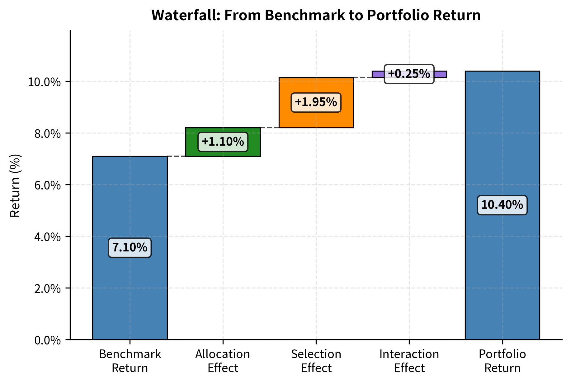
Worked Example
Let's implement Brinson attribution for a simple three-sector portfolio.
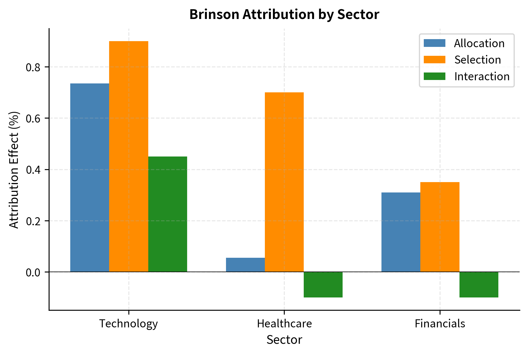
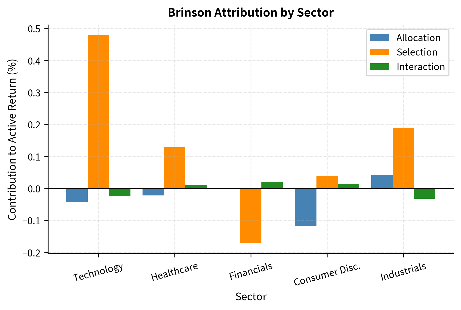
The attribution reveals that most of the portfolio's {python} f"{active_return:.2%}" outperformance came from selection effect ({python} f"{total_selection:.2%}"), indicating strong security selection across sectors. The positive allocation effect ({python} f"{total_allocation:.2%}") shows that overweighting technology (which outperformed) added value. The interaction effect ({python} f"{total_interaction:.2%}") reflects the benefit of combining good allocation with good selection, particularly in the technology sector where the portfolio both overweighted the sector and outperformed within it.
Visualization of Attribution Effects
Factor-Based Attribution
While Brinson attribution uses holdings data to decompose returns by sector, factor-based attribution uses returns data to decompose performance by exposure to systematic risk factors. This approach, rooted in the factor models we explored in Part IV Chapter 3, separates returns into two components: the portion explained by factor exposures (beta) and the residual unexplained by factors (alpha).
From CAPM to Multi-Factor Attribution
Building on our understanding of the CAPM from Part IV Chapter 2, recall that expected returns are determined by exposure to market risk. The CAPM posits a linear relationship between expected excess returns and market beta, establishing the foundational insight that investors are compensated for bearing systematic risk:
where:
- : expected return of asset
- : risk-free rate
- : sensitivity of asset to market movements
- : expected market return
This equation tells us that in equilibrium, the only source of expected excess returns should be exposure to market risk. Any return above or below this expectation represents either luck or skill. In an attribution context, we transition from this expectation to analyzing realized returns, which allows us to decompose actual performance into its constituent sources.
The realized return version of the CAPM transforms the equilibrium relationship into a regression framework:
where:
- : realized return of asset
- : risk-free rate
- : alpha (excess return unexplained by beta)
- : realized market beta
- : realized market return
- : idiosyncratic error term
This regression equation provides the foundation for factor-based attribution. The term represents the return attributable to market exposure, capturing the portion of returns that any investor could have earned simply by taking on market risk. The intercept represents the average return unexplained by market exposure, the "alpha" that active managers seek to generate. If is statistically significant and positive, it suggests the manager added value beyond simply taking market risk.
The residual term captures the period-by-period deviation from the linear relationship, representing idiosyncratic returns that are neither systematic nor persistent. This component averages to zero over time (by construction of OLS) and represents noise rather than skill.
Multi-factor models extend this decomposition to multiple sources of systematic risk, recognizing that the market factor alone does not capture all priced risks. Using the Fama-French three-factor model as an example, we add size and value factors to provide a richer characterization of systematic return drivers:
where:
- : realized asset return and risk-free rate
- : alpha (excess return unexplained by factor exposures)
- : exposure to market risk
- : realized market return
- : exposure to size premium (Small Minus Big)
- : exposure to value premium (High Minus Low)
- : returns of the size and value factors
- : idiosyncratic error term
Each beta coefficient measures the portfolio's sensitivity to a particular factor. A positive SMB beta indicates a tilt toward smaller companies, while a negative HML beta suggests a growth orientation. These exposures determine how much of the portfolio's return can be attributed to each systematic factor.
Factor-based attribution then decomposes total return into:
- Market contribution: \beta^{\text{MKT}}(R_m - R_f)
- Size contribution: \beta^{\text{SMB}} \cdot \text{SMB}
- Value contribution: \beta^{\text{HML}} \cdot \text{HML}
- Alpha: \alpha (residual skill)
This decomposition answers a critical question: how much of the portfolio's return came from passive exposure to known risk factors versus genuine security selection or market timing skill? A portfolio with high factor contributions and low alpha is essentially providing factor exposure, which can be replicated cheaply through index funds or smart beta products. A portfolio with significant alpha after controlling for factors demonstrates skill that may justify higher fees.
Estimating Factor Exposures
Factor exposures are estimated using time-series regression, as covered in Part III Chapter 19. The regression framework treats factor returns as explanatory variables and portfolio excess returns as the dependent variable, allowing us to estimate the sensitivity of the portfolio to each factor.
Given periods of return data, we regress portfolio excess returns on factor returns:
where:
- : portfolio excess return at time
- : intercept (estimated alpha)
- : factor loadings
- : factor returns at time
- : residual return at time
The OLS estimates provide both the factor loadings and an estimate of alpha with associated standard errors for statistical inference. The standard errors enable hypothesis testing, allowing us to assess whether each coefficient, including alpha, is statistically distinguishable from zero.
The regression framework offers several advantages for attribution. First, it requires only return data rather than detailed holdings information, making it applicable to hedge funds and other vehicles that do not disclose positions. Second, it automatically accounts for correlations between factors through the multivariate regression framework. Third, it provides statistical inference capabilities that allow us to quantify uncertainty around our estimates.
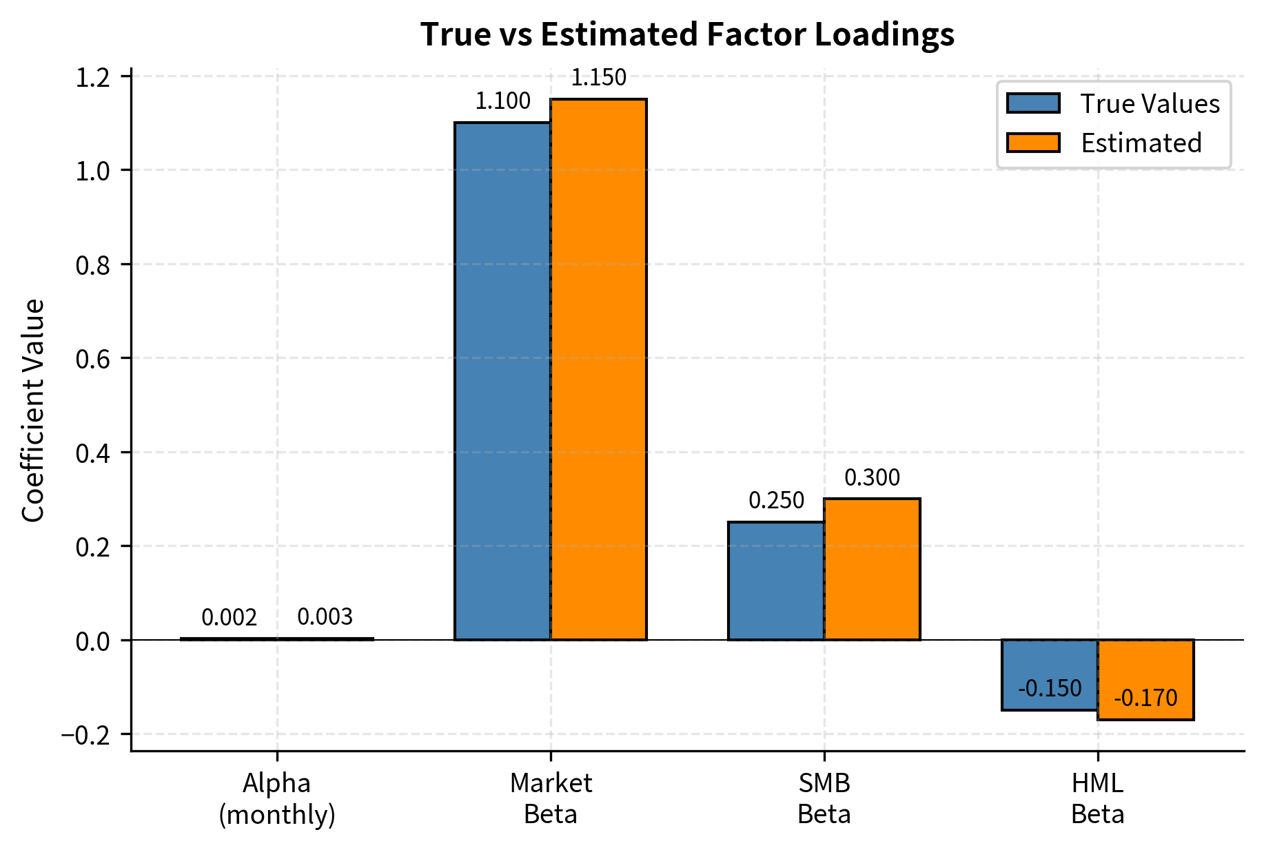
Implementation with Simulated Data
Let's implement factor-based attribution using a realistic simulation of portfolio returns.
The regression recovers factor exposures close to the true values (given estimation noise). The R-squared of around 70-80% indicates that the three factors explain most of the portfolio's return variation, with the remainder being idiosyncratic. The alpha estimate and its t-statistic allow us to assess whether the manager added value beyond factor exposures.
Return Attribution by Factor
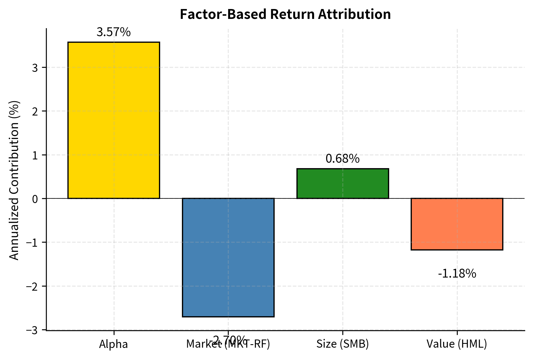
With the factor loadings estimated, we can decompose realized returns into contributions from each factor.
The annualized attribution reveals that the Market factor is the largest contributor to returns, driven by the portfolio's beta. The positive Alpha component indicates value added beyond these systematic drivers, while the Size and Value contributions reflect the specific factor tilts in the portfolio strategy.
Visualization of Factor Contributions
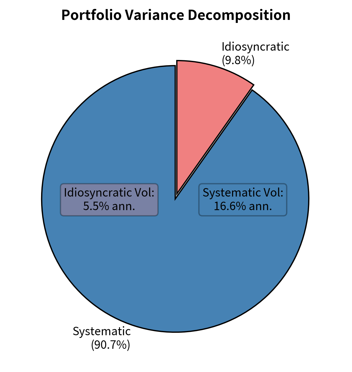
Risk Attribution
Beyond return attribution, factor models also allow us to attribute portfolio risk (variance) to factor sources. This analysis answers a complementary question: where does portfolio volatility come from?
The mathematical foundation for risk attribution relies on a key property of OLS regression. Because the regression residuals are uncorrelated with the factors by construction of ordinary least squares, the variance of the sum equals the sum of the variances. This orthogonality allows us to cleanly separate systematic from idiosyncratic risk.
Thus, the total variance decomposes into systematic and idiosyncratic components:
where:
- : total variance of portfolio excess returns
- : vector of factor loadings
- : factor covariance matrix
- : idiosyncratic variance
The first term, , captures systematic variance arising from factor exposures. This quadratic form accounts not only for each factor's individual variance but also for the correlations between factors. When factors are positively correlated, systematic risk may be amplified; when negatively correlated, they may partially offset. The second term, , represents idiosyncratic variance that cannot be attributed to any factor, reflecting security-specific risks that diversify away in large portfolios.
Key Parameters
The key parameters for factor-based attribution are:
- Alpha (): The intercept of the regression, representing returns unexplained by factor exposures.
- Betas (): Factor loadings measuring the sensitivity of the portfolio to each factor.
- Factors (): Systematic risk drivers (Market, Size, Value).
- Residuals (): Idiosyncratic returns specific to the portfolio.
Risk attribution reveals what percentage of portfolio volatility comes from factor exposures versus stock-specific risk. A portfolio with high systematic variance is primarily driven by factor movements, while high idiosyncratic variance suggests more active, stock-specific bets.
Separating Alpha from Beta
The central question in performance attribution is whether a manager's returns come from genuine skill (alpha) or simply from taking on compensated risk exposures (beta). This distinction has profound implications for evaluating investment managers and setting fee expectations.
The Alpha Illusion
A manager who consistently outperforms a simple benchmark like the S&P 500 might appear skilled, but factor analysis often reveals that the outperformance comes from systematic tilts rather than security selection skill. Consider a fund that overweights small-cap value stocks. When measured against a large-cap benchmark, this fund might show positive alpha. However, when measured against a model that includes size and value factors, the alpha may disappear entirely.
This phenomenon occurs because the fund's returns are explained by exposure to the size premium (the historical tendency of small stocks to outperform large stocks) and the value premium (the historical tendency of cheap stocks to outperform expensive stocks). Once we account for these factor tilts, there may be no residual alpha left, indicating that the manager was essentially providing factor exposure rather than demonstrating security selection skill.
The measured alpha depends critically on which factors are included in the benchmark model. Alpha relative to CAPM may become beta relative to a richer factor model. This is sometimes called the "alpha-beta boundary problem." The boundary between alpha and beta shifts as we expand our factor universe.
This observation doesn't mean the manager lacks skill; it means the skill lies in factor timing or factor selection rather than pure security selection. The key question becomes: are the factor tilts intentional and persistent, or are they incidental to an underlying stock-picking process?
Statistical Significance of Alpha
Even when alpha is present in a regression, we must assess whether it is statistically distinguishable from zero. Financial returns are noisy, and a positive alpha estimate might simply reflect sampling variation rather than true skill. The t-statistic for alpha provides a formal test of the null hypothesis that true alpha equals zero:
where:
- : t-statistic for the alpha estimate
- : estimated alpha
- : standard error of the alpha estimate
The t-statistic measures how many standard errors the estimated alpha lies from zero. Under the null hypothesis of zero alpha, the t-statistic follows a t-distribution, allowing us to calculate the probability of observing such an extreme estimate by chance alone.
A common threshold is , corresponding roughly to 95% confidence. However, given the multiple testing problem when evaluating many managers, more stringent thresholds (e.g., ) are often appropriate. When investors evaluate hundreds or thousands of fund managers, some will appear to have significant alpha purely by chance. Adjusting for multiple testing requires higher significance thresholds to maintain confidence in our conclusions.
These results indicate whether the manager's excess return is statistically distinguishable from zero. A p-value above 0.05 suggests that we cannot rule out luck as the source of outperformance, which is common in short datasets.
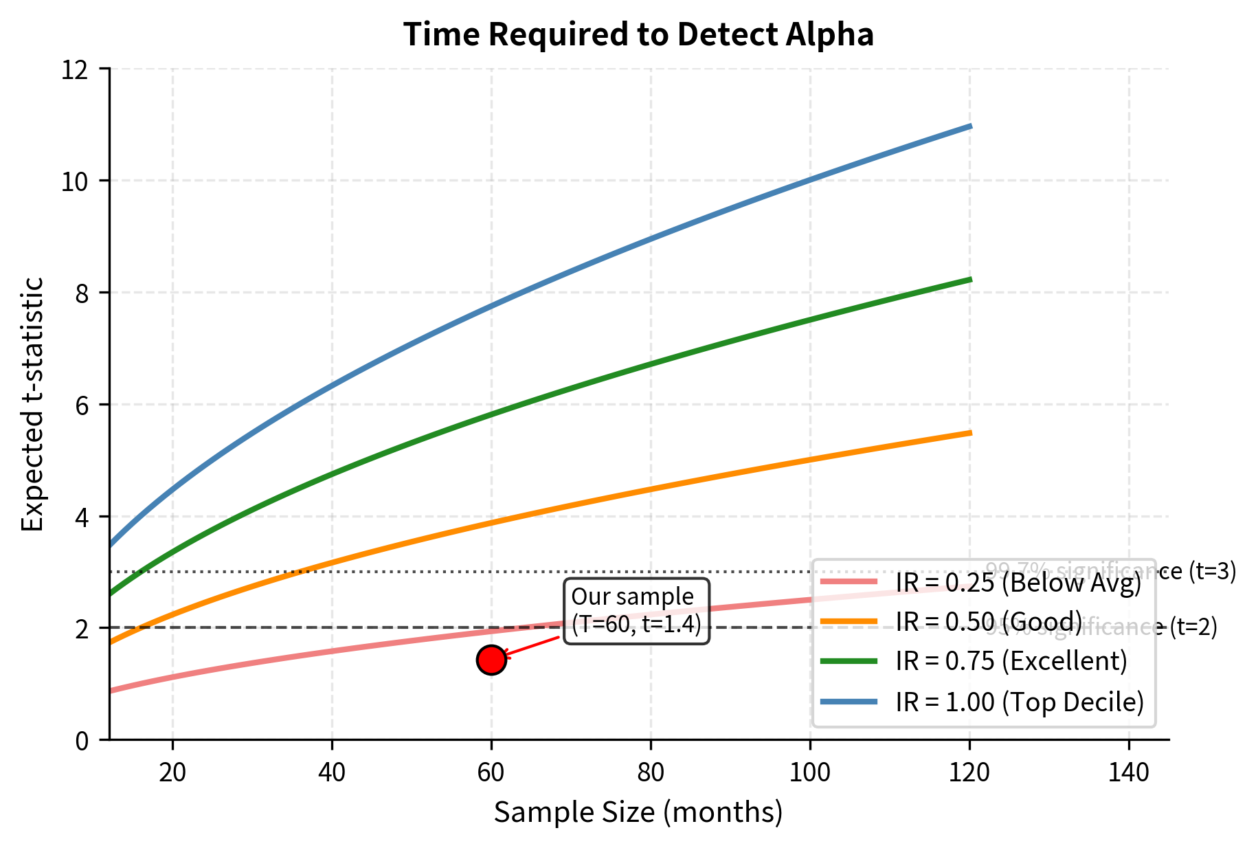
The Information Ratio Revisited
As we discussed in Portfolio Performance Measurement, the information ratio measures risk-adjusted active returns. This metric combines the magnitude of alpha with the consistency of that alpha, providing a more complete picture of manager skill than alpha alone:
where:
- : information ratio
- : active return or alpha
- : tracking error (residual volatility)
The numerator captures the average excess return generated, while the denominator measures the volatility of that excess return. A high information ratio indicates that the manager generates consistent alpha with relatively little noise, while a low information ratio suggests that any alpha comes with substantial uncertainty.
The information ratio can be estimated directly from the factor regression, and its t-statistic is related to the alpha t-statistic through a simple relationship:
where:
- : t-statistic of alpha
- : information ratio
- : number of time periods in the sample
This relationship reveals why detecting alpha requires sufficient data. The t-statistic grows with the square root of sample size, meaning that even a truly skilled manager needs many observations before their alpha becomes statistically significant. A manager with a true IR of 0.5 (considered excellent in the industry) needs roughly 16 observations to achieve a t-statistic of 2. With monthly data, this translates to over a year of track record just to reach marginal significance.
The Information Ratio puts the active return in the context of risk taken. The consistency between the expected and actual t-statistics demonstrates the mathematical link between risk-adjusted returns (IR) and statistical significance.
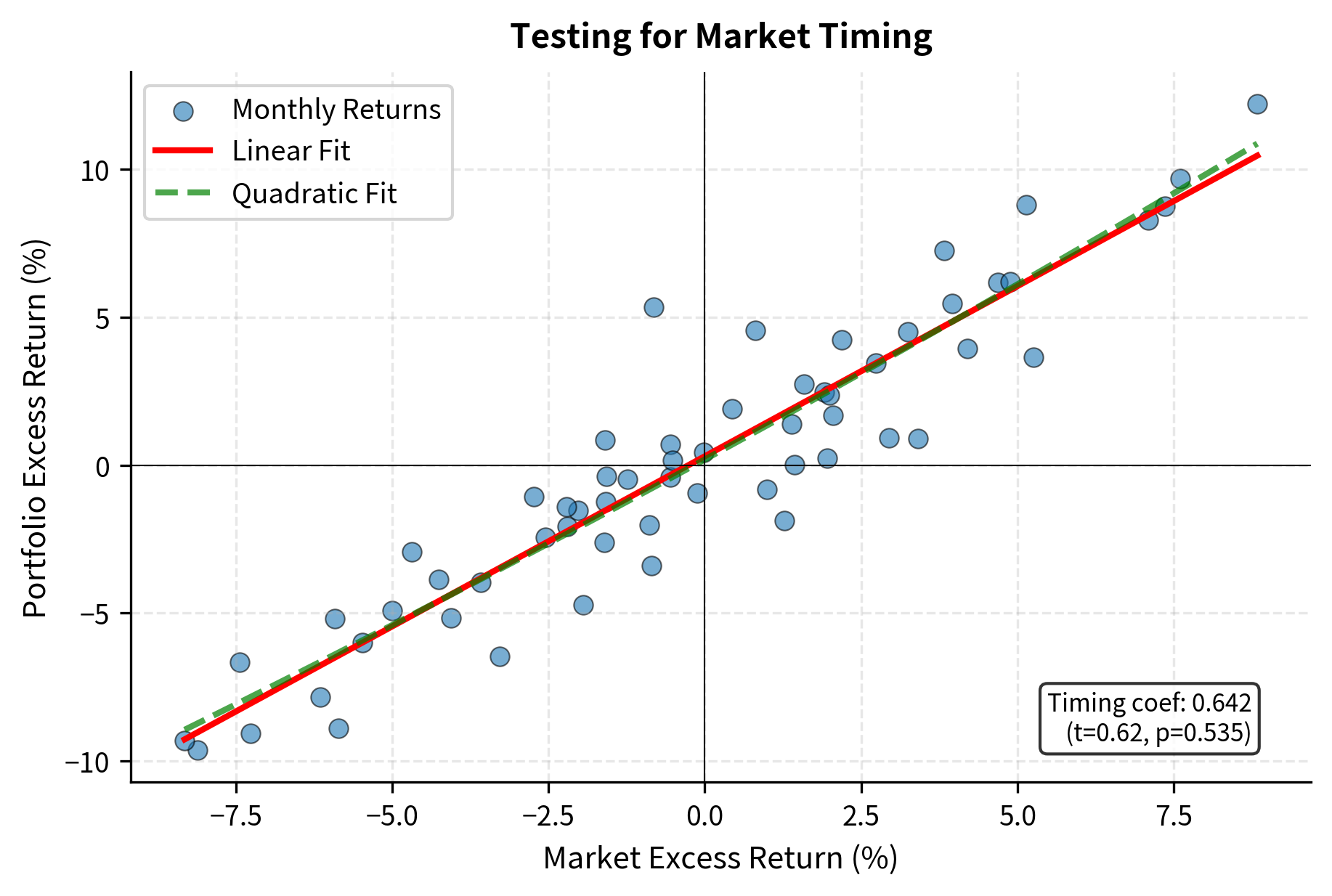
Alpha Decomposition: Timing vs. Selection
For equity portfolios, alpha can be further decomposed into components attributable to different skill types. This decomposition helps us understand not just whether a manager generates alpha, but how they generate it.
Security selection alpha measures the value added from choosing securities that outperform their factor-predicted returns. This is the alpha captured in our standard factor regression, representing the manager's ability to identify mispriced securities relative to their factor exposures.
Factor timing alpha measures value added from varying factor exposures over time. A manager who increases market beta before market rallies and decreases it before downturns exhibits market timing ability. Unlike selection alpha, timing alpha comes from adjusting exposures rather than from individual security choices.
We can test for timing ability by extending the factor model to include nonlinear terms. The key insight is that a successful market timer has a convex payoff profile: they participate more in up markets and less in down markets. This convexity can be captured by adding a squared market return term:
where:
- : portfolio excess return
- : alpha (selection skill)
- : market beta
- : market timing coefficient (curvature)
- : market excess return
- : squared market excess return
- : residual term
A positive and significant indicates positive market timing (convex payoff structure). When the market rises, the squared term is large and positive, contributing positively to returns if gamma is positive. When the market falls, the squared term is also positive (since squares are always positive), but the magnitude is smaller for mild declines. The net effect is a convex, option-like payoff that benefits from correctly anticipating market direction.
This approach, proposed by Treynor and Mazuy, extends naturally to multiple factors. We can add squared terms for each factor to test for timing ability with respect to size, value, or any other factor exposure.
Since we simulated returns without timing ability, we expect the timing coefficient to be statistically insignificant, which confirms our model correctly detects the absence of timing skill.
Comprehensive Attribution Example
Let's bring together Brinson and factor-based attribution in a comprehensive analysis that demonstrates how both frameworks complement each other.
Interpreting Attribution Results
The Brinson analysis reveals that the portfolio's {python} f"{total_active:.2%}" outperformance came primarily from two sources. First, the strong allocation effect in Technology ({python} f"{alloc[0]:+.2%}") resulted from overweighting a sector that outperformed the overall benchmark. Second, the selection effect reflects stock picks that beat sector benchmarks, with Technology ({python} f"{selec[0]:+.2%}") and Industrials ({python} f"{selec[4]:+.2%}") contributing most positively, though this was partially offset by underperformance in Financials ({python} f"{selec[2]:+.2%}").
From a factor perspective, a manager might further analyze whether the Technology outperformance came from factor tilts within tech (e.g., overweighting growth-oriented tech stocks) or from genuine stock selection orthogonal to known factors. This level of analysis requires combining holdings data with factor exposure data, a technique used by sophisticated institutional investors.
Practical Applications and Challenges
Performance attribution serves diverse needs across the investment management ecosystem, from evaluating managers to improving investment processes. This section examines common use cases and the practical challenges that arise when implementing attribution frameworks.
Use Cases for Performance Attribution
Performance attribution serves multiple constituencies in the investment management ecosystem:
Asset owners (pension funds, endowments) use attribution to evaluate whether managers are delivering on their stated investment approach. A value manager who generates returns primarily through market timing rather than value stock selection may not be providing the exposure the investor intended.
Investment managers use attribution internally to improve their investment process. Attribution can reveal whether a team's research is translating into profitable stock selection or whether returns are coming from unintended factor bets.
Risk managers use factor attribution to understand the sources of portfolio volatility and ensure that risk is being taken intentionally and in line with mandates.
Consultants use attribution to compare managers on a risk-adjusted, factor-adjusted basis, enabling more meaningful peer comparisons.
Challenges in Practice
Several practical challenges complicate real-world attribution analysis.
Data quality and timing present significant hurdles. Brinson attribution requires accurate holdings data at consistent timestamps. Portfolio holdings may be reported monthly or quarterly, while prices move continuously, creating potential timing mismatches.
Benchmark selection critically affects results. The choice of benchmark determines what counts as active management. An inappropriate benchmark can make passive factor exposure appear as alpha or mask genuine skill.
Factor model specification affects factor-based attribution similarly. As noted earlier, alpha is model-dependent. The proliferation of factors (some research identifies hundreds of "anomalies") raises questions about which factors to include. Including too many factors may attribute true alpha to spurious factors; including too few may miss systematic exposures.
Statistical reliability remains a persistent challenge. Short track records make it difficult to distinguish skill from luck. Even five years of monthly data provides only 60 observations, often insufficient to confidently estimate alpha, especially given the noise in financial returns.
Time-varying exposures complicate interpretation. Factor loadings and sector weights change over time as managers adjust their portfolios. Static regression may mischaracterize a manager whose style has evolved, requiring rolling-window or time-varying parameter approaches.
Beyond Single-Period Attribution
Real-world attribution often requires analyzing performance over extended periods. Multi-period attribution compounds single-period effects, but compounding creates challenges. The interaction between allocation and selection across time periods generates additional terms. Various linking methods (multiplicative, logarithmic) exist to address this, each with different properties.
For factor-based attribution over time, rolling-window regressions can capture changing factor exposures. However, this introduces a tradeoff between responsiveness (shorter windows) and statistical precision (longer windows).
Limitations and Impact
Performance attribution has fundamentally changed how the investment industry evaluates managers and allocates capital. By enabling precise decomposition of returns, attribution has exposed many previously "skilled" managers as factor investors, driving a massive shift toward lower-cost factor-based strategies. The rise of smart beta and factor investing owes much to attribution analysis revealing that a significant portion of active management returns can be replicated through systematic factor exposure.
However, attribution has notable limitations that practitioners must understand. The backward-looking nature of attribution means it explains past returns but doesn't necessarily predict future performance. A manager who generated alpha historically may have been lucky, or their edge may have been arbitraged away. Attribution also cannot distinguish between skill and uncompensated risk-taking. A manager who concentrates in a few stocks might generate alpha simply by taking on unpriced idiosyncratic risk that happened to pay off.
The factor zoo problem presents another challenge. With hundreds of published factors, there's a risk of overfitting attribution models, finding factors that explain past returns spuriously without reflecting genuine systematic risk premia. This concern has led to greater scrutiny of factor robustness and out-of-sample validity.
Despite these limitations, performance attribution remains an indispensable tool. When combined with qualitative assessment of investment process, appropriate benchmark selection, and statistical rigor, attribution provides essential insights into the sources of investment performance. As we explore advanced portfolio construction techniques in the next chapter, we'll see how attribution insights inform portfolio optimization and factor targeting strategies.
Summary
This chapter developed two complementary frameworks for understanding the sources of portfolio performance:
Brinson attribution decomposes active returns into allocation, selection, and interaction effects based on portfolio holdings and sector weights. Allocation effect measures value added from over- or underweighting sectors, while selection effect captures the contribution from security picks within each sector. The interaction effect accounts for the combined benefit of both overweighting a sector and outperforming within it.
Factor-based attribution uses regression analysis to separate returns into systematic factor exposures (beta) and residual alpha. This approach leverages the factor models developed earlier in Part IV to determine how much return comes from market exposure, size tilts, value tilts, and other systematic factors versus genuine stock selection skill.
The distinction between alpha and beta lies at the heart of investment management. True alpha, returns uncorrelated with known factors, represents genuine investment skill and justifies active management fees. However, alpha is model-dependent, and statistical significance requires long track records. What appears as alpha under simple benchmarks often becomes beta when analyzed against richer factor models.
Practical applications include manager evaluation, investment process improvement, risk attribution, and fee negotiations. Challenges include data quality, benchmark selection, factor model specification, and the fundamental difficulty of distinguishing skill from luck given the noise in financial returns.
Performance attribution has driven significant industry changes, including the growth of factor investing and increased scrutiny of active management fees. While backward-looking and subject to model specification choices, attribution remains essential for understanding investment performance and making informed allocation decisions.
Quiz
Ready to test your understanding? Take this quick quiz to reinforce what you've learned about performance attribution and investment alpha.

Comments