

Master Sharpe ratio, Sortino ratio, information ratio, and maximum drawdown metrics. Learn to evaluate portfolios with Python implementations.
Choose your expertise level to adjust how many terms are explained. Beginners see more tooltips, experts see fewer to maintain reading flow. Hover over underlined terms for instant definitions.
Portfolio Performance Measurement
Constructing a portfolio is only half the challenge in quantitative finance. The other half is answering a deceptively simple question: how well did it actually perform? Raw returns tell an incomplete story. A fund that gained 20% sounds impressive until you learn it took on three times the market's risk to achieve it, or that it suffered a 50% loss along the way before recovering. Portfolio performance measurement provides the analytical framework to evaluate investment results rigorously, accounting for the risk taken, the benchmark against which performance should be judged, and the path returns took to reach their final value.
This chapter develops the core metrics used by portfolio managers, allocators, and risk officers to assess investment performance. Building on the mean-variance framework from our discussion of Modern Portfolio Theory and the factor models introduced with CAPM and APT, we now turn to measuring how well these theoretical constructs translate into realized results. You'll learn to compute risk-adjusted returns using the Sharpe and information ratios, quantify downside risk through maximum drawdown and the Calmar ratio, and properly benchmark active strategies against their relevant indices. These tools are essential not only for evaluating past performance but also for making informed allocation decisions going forward.
Risk-Adjusted Return Metrics
Raw returns are seductive in their simplicity but misleading in isolation. A hedge fund returning 15% annually might seem superior to one returning 10%, but if the first fund achieves this with twice the volatility, the risk-return tradeoff may actually favor the second. This observation reveals a fundamental truth about investment evaluation: returns cannot be judged in a vacuum. Every return comes attached to a risk profile, and meaningful comparison requires understanding both dimensions simultaneously.
Risk-adjusted return metrics address this by normalizing returns against some measure of risk, enabling meaningful comparisons across strategies with different risk profiles. The central insight driving these metrics is that investors should be rewarded for taking risk, so we need to measure how efficiently each unit of risk translates into return. A strategy that generates high returns through high risk may actually be less attractive than a moderate-return strategy with low risk, depending on how the risk and return scale together.
The Sharpe Ratio
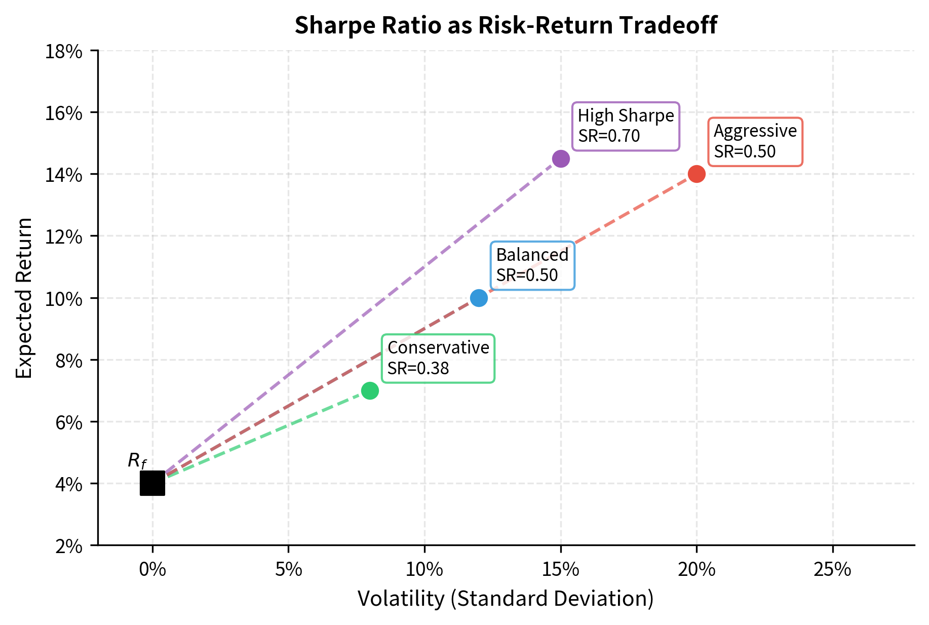
The Sharpe ratio, introduced by William Sharpe in 1966, remains the most widely used risk-adjusted performance measure in finance. Its enduring popularity stems from both its intuitive appeal and its theoretical foundation in mean-variance portfolio theory. The ratio quantifies the excess return earned per unit of total risk, where total risk is measured by the standard deviation of returns. In essence, it answers a simple but powerful question: how much additional compensation does an investor receive for accepting the uncertainty inherent in the investment?
The Sharpe ratio measures the average excess return per unit of volatility. It answers the question: how much additional return does the portfolio generate for each unit of total risk taken?
To understand why the Sharpe ratio takes its particular form, consider the investment decision from a rational investor's perspective. Any investor has the option to earn the risk-free rate with certainty by holding Treasury bills or similar instruments. When an investor chooses a risky portfolio instead, they demand compensation for accepting uncertainty. This compensation takes the form of expected returns above the risk-free rate. The Sharpe ratio measures how efficiently the portfolio converts risk into this risk premium.
The mathematical formulation is straightforward. For a portfolio with returns and a risk-free rate , the Sharpe ratio is:
where:
- : expected portfolio return
- : risk-free rate
- : standard deviation of portfolio returns
The numerator represents the risk premium: the expected return in excess of what could be earned risk-free. This quantity captures the reward component of the risk-reward tradeoff. The denominator measures total volatility, encompassing all sources of return variation regardless of whether they stem from market movements, idiosyncratic factors, or any other source of uncertainty. By dividing reward by risk, the Sharpe ratio produces a standardized measure that allows direct comparison between portfolios with vastly different risk levels.
When working with historical data, we estimate these quantities from realized returns rather than theoretical expectations. The transition from population parameters to sample statistics introduces estimation uncertainty, but the basic structure remains the same. Given return observations , the sample Sharpe ratio becomes:
where:
- : sample mean return
- : risk-free rate
- : sample standard deviation
- : number of return observations
- : portfolio return in period
The sample mean replaces the expected value, and the sample standard deviation replaces the population volatility. Notice that we use in the denominator of the sample standard deviation to correct for bias when estimating variance from a sample. This Bessel's correction ensures that our volatility estimate is unbiased, which becomes particularly important when working with shorter time series.
Annualization is critical when comparing Sharpe ratios computed from different return frequencies. Investment returns are observed at various frequencies, from high-frequency intraday data to annual reports, and comparing Sharpe ratios across these frequencies requires careful scaling. The key insight is that returns and volatilities scale differently with time: expected returns scale linearly with the number of periods, while standard deviations scale with the square root of time (assuming returns are independent).
If you have monthly returns with mean excess return and standard deviation , the annualized Sharpe ratio is:
where:
- : mean monthly excess return
- : standard deviation of monthly returns
- : number of months in a year
The derivation proceeds by recognizing that annualizing the monthly mean requires multiplying by 12 (twelve months of returns accumulate), while annualizing the monthly standard deviation requires multiplying by (volatility grows with the square root of time under the assumption of independent returns). When we take the ratio, the annualization factors partially cancel, leaving only as the multiplicative adjustment.
The general formula for annualizing from any frequency is:
where:
- : Sharpe ratio calculated using periodic returns
- : number of periods per year (e.g., 12 for monthly, 252 for daily)
This scaling relationship has an important implication: the annualization factor amplifies the periodic Sharpe ratio. A daily Sharpe ratio of 0.05 becomes an annualized Sharpe ratio of approximately 0.79 when multiplied by . This amplification effect means that small daily edges, when compounded over many trading days, can produce attractive annualized risk-adjusted returns.
Interpretation of Sharpe ratio values varies by context, but general benchmarks exist that help practitioners calibrate their expectations:
- SR < 0: The portfolio underperforms the risk-free rate
- 0 < SR < 0.5: Poor risk-adjusted returns
- 0.5 < SR < 1.0: Acceptable risk-adjusted returns
- 1.0 < SR < 2.0: Good risk-adjusted returns
- SR > 2.0: Excellent, though often unsustainable or based on limited data
These benchmarks should be applied with appropriate skepticism. A Sharpe ratio above 2.0, while theoretically possible, should prompt careful investigation. Such high ratios are difficult to sustain over long periods and may indicate data errors, survivorship bias, or strategies that work in backtests but fail in live trading. Similarly, a negative Sharpe ratio signals that the investor would have been better off in risk-free assets, suggesting the strategy provides inadequate compensation for the risks involved.
The Sortino Ratio
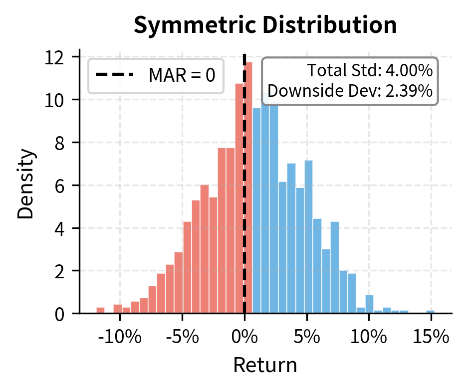
The Sharpe ratio treats upside and downside volatility identically, which may not align with investor preferences. Most investors are not troubled by positive surprises; they care about downside risk. When a portfolio unexpectedly gains 10%, investors celebrate rather than complain about volatility. The asymmetry in how investors experience gains versus losses motivates an alternative risk measure that focuses specifically on the volatility that investors actually want to avoid.
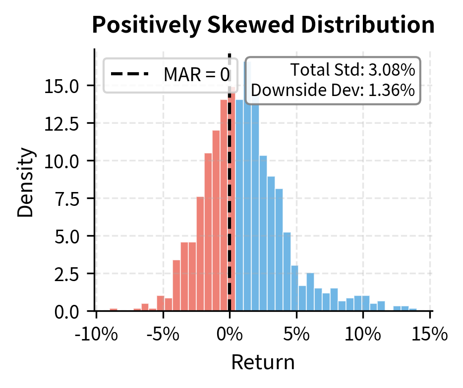
The Sortino ratio addresses this asymmetry by replacing total volatility with downside deviation. Rather than penalizing a strategy for all return variation, the Sortino ratio penalizes only negative deviations from a target return. This distinction becomes particularly important for strategies with asymmetric return distributions, where the standard deviation may poorly represent the actual downside risk investors face.
Downside deviation measures the volatility of returns that fall below a specified minimum acceptable return (MAR), typically zero or the risk-free rate. It captures only the "bad" volatility that investors want to avoid.
The concept of a minimum acceptable return provides flexibility in defining what constitutes unacceptable performance. For some investors, any negative return is unacceptable, leading to a MAR of zero. For others, failing to beat the risk-free rate represents underperformance, suggesting the risk-free rate as the appropriate MAR. Institutional investors may set the MAR equal to their liability growth rate or an actuarial assumption. The choice of MAR reflects the investor's specific circumstances and objectives.
The Sortino ratio is defined as:
where:
- : expected portfolio return
- : minimum acceptable return
- : downside deviation
The numerator measures the expected return above the minimum acceptable threshold, which represents the reward investors seek. The denominator captures only the volatility of returns falling below this threshold, focusing the risk measure on outcomes that investors view as failures. This construction ensures that positive surprises do not inflate the risk measure, which would inappropriately penalize desirable outcomes.
The downside deviation is computed as:
where:
- : total number of observations
- : return in period
- : minimum acceptable return
- : function filtering for negative deviations (returns below MAR)
Note that only returns below the MAR contribute to this calculation. Returns above the threshold contribute zero to the sum. The minimum function ensures that positive deviations (returns exceeding the MAR) are replaced by zero before squaring, effectively filtering out the "good" volatility that investors welcome.
An important computational detail is that we divide by , the total number of observations, rather than just the number of negative observations. This choice ensures that strategies with fewer downside events are appropriately rewarded with lower downside deviation, reflecting the reality that they expose investors to less frequent downside risk.
The Sortino ratio will always be greater than or equal to the Sharpe ratio for portfolios with positive skewness (more upside than downside), but the gap narrows for negatively skewed returns where downside volatility dominates. This property makes the Sortino ratio particularly useful for evaluating strategies that explicitly aim for asymmetric return profiles, such as option-based strategies or trend-following systems. A strategy that buys options, for instance, has limited downside (the premium paid) but unlimited upside. Its Sharpe ratio might look mediocre due to the volatility from occasional large gains, while its Sortino ratio would more accurately reflect its attractive downside characteristics.
Benchmarking and Active Management Metrics
While the Sharpe ratio measures absolute risk-adjusted performance, many investment mandates are defined relative to a benchmark. An equity portfolio manager might be evaluated against the S&P 500, a bond manager against the Bloomberg Aggregate Bond Index. For these mandates, outperforming the benchmark matters more than absolute return, and the relevant metrics shift accordingly. The question transforms from "Did the portfolio generate attractive risk-adjusted returns?" to "Did the portfolio generate better returns than an investor could have achieved by simply holding the benchmark?"
This relative perspective reflects the practical reality of delegated portfolio management. When an investor hires an active manager, they pay fees for the manager's expertise. The relevant counterfactual is not earning the risk-free rate but rather holding a passive benchmark, which is now available at extremely low cost through index funds and ETFs. The value added by active management must therefore be measured relative to this accessible alternative.
Active Return and Tracking Error
Active return is the difference between the portfolio's return and its benchmark's return over the same period:
where:
- : portfolio return
- : benchmark return
This straightforward calculation answers the most basic question about active management: did the portfolio outperform? A positive active return indicates outperformance, while a negative active return indicates underperformance. However, like raw returns, active returns in isolation provide an incomplete picture because they ignore the risk taken to achieve them.
This quantity is also called the excess return relative to the benchmark, though this terminology can cause confusion with the excess return over the risk-free rate used in the Sharpe ratio. To avoid ambiguity, many practitioners use "active return" when discussing benchmark-relative performance and reserve "excess return" for returns above the risk-free rate. Being precise about terminology is particularly important when communicating with clients or colleagues who may use these terms differently.
Tracking error, also known as active risk, measures the volatility of these active returns:
where:
- : standard deviation operator
- : variance operator
- : active return series
Tracking error captures a fundamentally different concept than portfolio volatility. While portfolio volatility measures total risk, tracking error measures the risk of deviating from the benchmark. A portfolio can have low tracking error but high absolute volatility (if it closely mimics a volatile benchmark) or high tracking error but low absolute volatility (if it diverges significantly from a volatile benchmark by holding cash).
Tracking error quantifies how consistently a portfolio tracks its benchmark. A passive index fund targeting zero tracking error will have very low TE (perhaps 0.1% annually), while an aggressive active manager might exhibit tracking error of 5% or more. The magnitude of tracking error reflects the degree of active decision-making: a manager who makes large sector bets, holds concentrated positions, or times the market will generate higher tracking error than a manager who makes modest tilts around benchmark weights.
From the variance properties we covered in the probability fundamentals chapter, we can decompose tracking error step-by-step to understand what drives its magnitude:
where:
- : standard deviations of portfolio and benchmark returns
- : correlation between portfolio and benchmark returns
- : portfolio and benchmark returns
This decomposition reveals the drivers of tracking error. The first two terms, , represent the combined volatility of the portfolio and benchmark. The third term, , reduces tracking error to the extent that portfolio and benchmark returns move together. When correlation is perfect () and volatilities are equal (), tracking error becomes zero because the portfolio and benchmark move in lockstep.
This analysis shows that tracking error increases when the portfolio diverges from the benchmark either through different volatility or lower correlation. A manager who holds very different securities from the benchmark will have low correlation and hence high tracking error. Similarly, a manager who uses leverage to amplify returns will have higher portfolio volatility and consequently higher tracking error even if the underlying positions correlate perfectly with the benchmark.
The Information Ratio
The Information ratio (IR) is the benchmark-relative analog of the Sharpe ratio. Just as the Sharpe ratio measures absolute returns per unit of absolute risk, the information ratio measures active returns per unit of active risk. It provides a standardized measure of whether a manager's deviation from the benchmark is rewarded with proportionate outperformance.
The information ratio is defined as:
where:
- : expected active return
- : average active return
- : tracking error (volatility of active returns)
The information ratio measures a manager's skill at generating returns above the benchmark relative to the risk taken in deviating from that benchmark. A higher IR indicates more consistent alpha generation.
The numerator, often denoted (alpha), represents the average outperformance relative to the benchmark. This is the value added by active management. The denominator, tracking error, represents the active risk taken to achieve this outperformance. By normalizing alpha by tracking error, the information ratio answers the crucial question: is the manager's outperformance large enough to justify the risk of deviating from the benchmark?
The information ratio answers a different question than the Sharpe ratio. The Sharpe ratio asks: "Is this portfolio's risk-reward profile attractive on an absolute basis?" The information ratio asks: "Is this manager adding value relative to simply holding the benchmark?" These questions have different implications depending on the investor's situation. An investor choosing between a hedge fund and Treasury bills cares about the Sharpe ratio. An investor choosing between an active manager and an index fund cares about the information ratio.
Interpretation benchmarks for the information ratio are:
- IR < 0: The manager destroys value relative to the benchmark
- 0 < IR < 0.5: Mediocre active management
- 0.5 < IR < 1.0: Good active management
- IR > 1.0: Exceptional active management (rare and difficult to sustain)
Research suggests that an information ratio above 0.5 sustained over a long period places a manager in the top quartile of active managers. This benchmark reflects the difficulty of consistently outperforming after fees and transaction costs. IRs above 1.0 are extremely rare and should be viewed with skepticism unless based on extensive track records. The few managers who achieve such high information ratios typically have some structural advantage, such as access to unique information, superior technology, or the ability to exploit market segments where competition is limited.
The Fundamental Law of Active Management
The information ratio connects directly to the skill and breadth of active investment decisions through the Fundamental Law of Active Management, developed by Richard Grinold. This elegant relationship decomposes the information ratio into two components: the quality of individual forecasts and the number of opportunities to apply those forecasts.
where:
- : Information Coefficient (correlation between forecasted and realized returns)
- : Breadth (number of independent investment decisions per year)
The Information Coefficient measures forecasting skill. It represents the correlation between a manager's predictions and subsequent realized returns. An IC of zero indicates no forecasting ability (predictions are uncorrelated with outcomes), while an IC of 1.0 would indicate perfect foresight. In practice, even skilled managers have ICs in the range of 0.02 to 0.10, reflecting the inherent difficulty of forecasting financial returns.
Breadth captures the number of independent opportunities to apply forecasting skill. A manager who makes one large bet per year has breadth of 1, while a manager who makes 100 independent security selection decisions has breadth of 100. The key word is "independent": if decisions are correlated, effective breadth is lower than the raw count.
This relationship has profound implications for investment strategy design. A manager with modest forecasting skill (IC = 0.05) making 100 independent bets per year achieves approximately the same IR as a manager with higher skill (IC = 0.10) making only 25 bets. Specifically, equals . The law suggests that diversifying across many independent opportunities can compensate for imperfect forecasting ability.
This insight explains why quantitative strategies that make many small bets across hundreds or thousands of securities can compete with concentrated stock pickers despite having lower conviction in any individual position. Your advantage comes from breadth, while the stock picker's advantage comes from depth of insight (higher IC on fewer positions). Both paths can lead to attractive information ratios, but they require different organizational structures and skill sets.

We'll explore this relationship further in the upcoming chapter on Performance Attribution and Investment Alpha, where we decompose manager skill into its component sources.
Drawdown Analysis
The metrics discussed so far focus on the distribution of returns without considering their sequence. Two portfolios with identical Sharpe ratios might have very different investor experiences if one suffered a catastrophic 60% drawdown mid-period while the other had a smooth path. Standard deviation treats a 10% gain followed by a 10% loss identically to a 10% loss followed by a 10% gain, but these sequences feel very different to an investor watching their account balance.
Drawdown analysis captures this path-dependent aspect of portfolio risk. It examines not just the volatility of returns but the specific patterns of losses, focusing on the magnitude and duration of peak-to-trough declines. For many investors, maximum drawdown is more psychologically salient than volatility because it represents the worst paper loss they would have experienced, a number that determines whether they would have had the discipline to stick with the strategy.
Maximum Drawdown
The drawdown at any point in time measures the percentage decline from the most recent peak. Conceptually, it answers the question: "If you had invested at the best possible time before now, how much would you have lost?" This perspective captures the regret an investor might feel having bought at a local maximum.
The drawdown at time is calculated relative to the high-water mark established up to that point:
where:
- : portfolio value at time
- : running maximum value (high-water mark) up to time
The numerator represents the difference between the highest value achieved so far and the current value. Dividing by the high-water mark expresses this difference as a percentage of the peak value. A drawdown of 0 means the portfolio is at a new high, while a drawdown of 0.20 means the portfolio has declined 20% from its peak.
The Maximum Drawdown (MDD) represents the largest drawdown observed over the entire evaluation period:
where:
- : drawdown at time
- : running maximum value (high-water mark) up to time
- : portfolio value at time
- : operator finding the maximum value over the entire time period
Maximum drawdown represents the largest peak-to-trough decline in portfolio value before a new peak is established. It measures the worst-case loss an investor would have experienced if they invested at the peak and sold at the trough.
Maximum drawdown captures tail risk that volatility-based measures may miss. The distinction becomes clear when considering strategies with different return distributions. A strategy with low volatility but occasional catastrophic losses (like selling deep out-of-the-money options) might have an attractive Sharpe ratio but terrifying maximum drawdown. The option seller collects small premiums regularly, generating consistent returns with low measured volatility. But when the rare catastrophic event occurs, losses can exceed all previous gains. The Sharpe ratio might show a respectable 0.8, while the maximum drawdown reveals a 40% or larger loss, exposing a risk that volatility alone cannot capture.
Drawdown Duration
Beyond the magnitude of drawdowns, their duration matters significantly for investor welfare. A quick 15% drawdown that recovers within a month is psychologically easier to endure than a 15% drawdown that takes two years to recover. The drawdown duration measures how long it takes to recover from a drawdown and establish a new high-water mark.
Key duration metrics include:
- Time to trough: The period from peak to the lowest point
- Recovery time: The period from trough back to a new peak
- Total drawdown duration: The sum of time to trough and recovery time
Each component provides distinct information about the nature of losses. Time to trough indicates how quickly losses accumulated, with faster declines often associated with market stress or forced liquidations. Recovery time indicates how long the strategy takes to regain lost ground, reflecting the magnitude of the required recovery (a 50% loss requires a 100% gain to recover) and the strategy's return characteristics during the recovery period.
Lengthy drawdowns can be psychologically devastating for investors, even if the eventual recovery is complete. A fund that takes three years to recover from a 20% drawdown may lose clients long before it reaches new highs. Investor patience is finite, and redemptions during drawdowns can force a manager to sell at unfavorable prices, potentially extending the drawdown further. Understanding both drawdown magnitude and duration helps investors set realistic expectations and managers design strategies compatible with their clients' time horizons.
The Calmar Ratio
The Calmar ratio combines return analysis with drawdown analysis by relating annualized return to maximum drawdown:
where:
- : compound annual growth rate of the portfolio
- : maximum peak-to-trough decline over the period
The Calmar ratio measures annualized return per unit of maximum drawdown risk. It rewards consistent performance and penalizes strategies that achieve returns through occasional catastrophic losses.
The Calmar ratio provides a fundamentally different perspective on risk-adjusted returns than the Sharpe ratio. While the Sharpe ratio uses volatility as the risk measure, which reflects the typical variability of returns, the Calmar ratio focuses on the worst historical loss. This distinction matters because volatility and maximum drawdown can tell very different stories about a strategy's risk profile.
A Calmar ratio of 1.0 means the annualized return equals the maximum drawdown. In this case, an investor can expect to earn returns roughly equal to the worst loss they might experience. A Calmar ratio of 2.0 means returns are twice the worst drawdown, suggesting more attractive compensation for drawdown risk. Conversely, a Calmar ratio of 0.5 means the worst drawdown is twice the annualized return, indicating that recovery from the worst loss could take two or more years even if future returns match historical averages.
The Calmar ratio is particularly favored by practitioners in managed futures and hedge fund evaluation, where maximum drawdown often defines client risk tolerance more directly than volatility. Many investors have specific drawdown limits: they will redeem from any manager who experiences a 20% drawdown, regardless of Sharpe ratio. For these investors, the Calmar ratio directly measures whether a strategy's return potential justifies its drawdown risk.
Interpretive benchmarks vary by strategy:
- Calmar < 0.5: Poor risk-adjusted returns relative to drawdown
- 0.5 < Calmar < 1.0: Acceptable
- 1.0 < Calmar < 2.0: Good
- Calmar > 2.0: Excellent
These benchmarks should be interpreted in context. Strategies that experience smaller maximum drawdowns will naturally tend to have higher Calmar ratios for a given level of returns. Comparing Calmar ratios across strategies with dramatically different drawdown characteristics requires careful judgment about whether the comparison is meaningful.
Computing Performance Metrics in Python
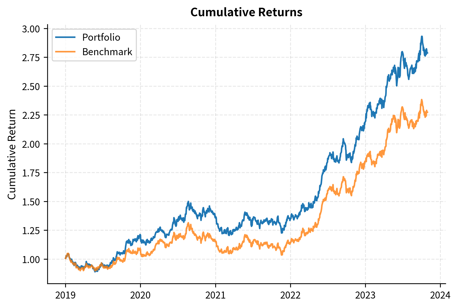
Let's implement these metrics and apply them to realistic portfolio data. We'll work with simulated returns that exhibit properties common in equity portfolios: modest positive drift, time-varying volatility, and occasional drawdowns.
First, we'll generate synthetic return series for a portfolio and its benchmark, simulating approximately five years of daily data.
Implementing the Sharpe Ratio
The portfolio's higher Sharpe ratio reflects both the embedded alpha and the independent tracking noise. A Sharpe ratio near 0.6-0.7 is realistic for a well-managed equity portfolio over a multi-year period.
Implementing the Sortino Ratio
The Sortino ratio exceeds the Sharpe ratio because our simulated returns are approximately symmetric. In practice, the relationship between these ratios reveals information about the skewness of the return distribution.
Implementing the Information Ratio
The information ratio of approximately 0.4-0.5 is consistent with a skilled active manager. The alpha is close to our simulated 2%, and tracking error matches the noise we introduced.
Implementing Drawdown Analysis
The maximum drawdown figures highlight the worst historical loss experienced by each strategy. The portfolio's maximum drawdown represents the deepest peak-to-trough decline, while the duration metric indicates the number of days required to recover from that loss. These metrics quantify the tail risk and psychological endurance required to stick with the strategy.
Implementing the Calmar Ratio
A Calmar ratio above 0.5 indicates that annualized returns exceed half the maximum drawdown, suggesting reasonable compensation for the drawdown risk experienced.
Visualizing Performance
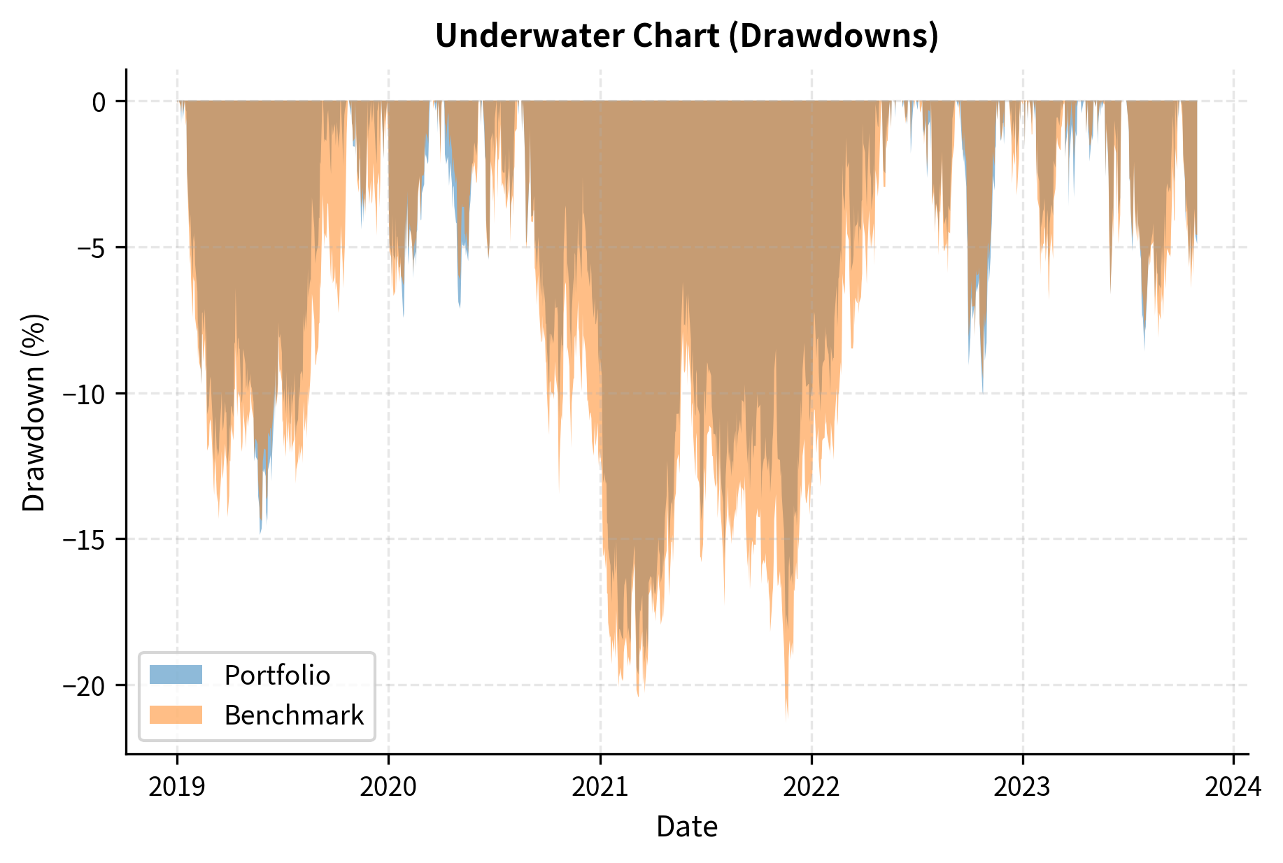
The underwater chart (below) provides an intuitive visualization of drawdowns. The depth shows magnitude while the width indicates duration. This view helps investors understand the path their capital took, not just the endpoint.
Performance Summary Dashboard
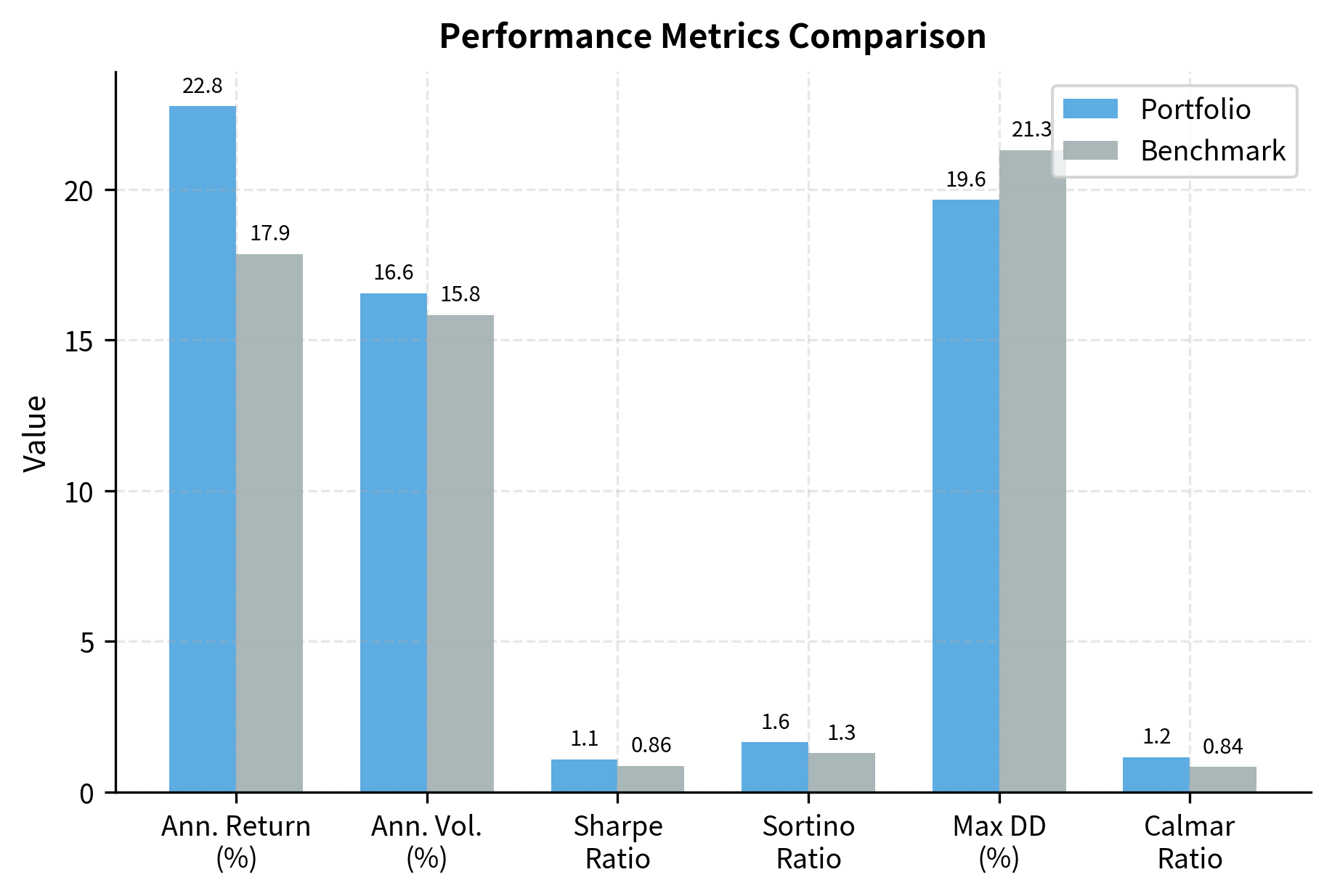
Let's consolidate all metrics into a comprehensive performance summary, which is standard practice for portfolio reporting.
This summary provides a comprehensive view of both absolute and relative performance. The portfolio demonstrates modest alpha generation with controlled tracking error, resulting in a positive information ratio.
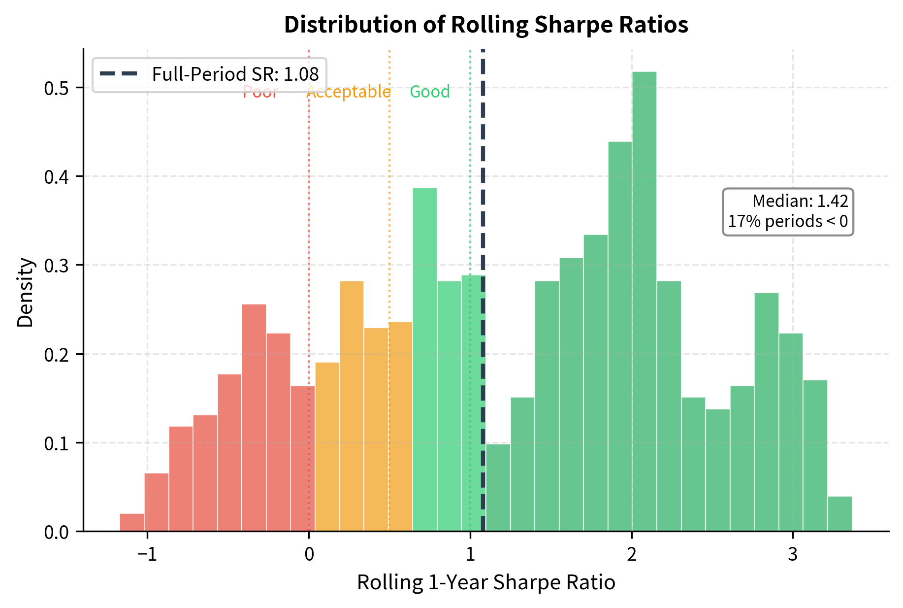
Rolling Performance Analysis
Static performance metrics over the full period can mask time-varying behavior. A manager might have excellent performance in one regime but poor performance in another. Rolling analysis captures this dynamic by computing metrics over moving windows.
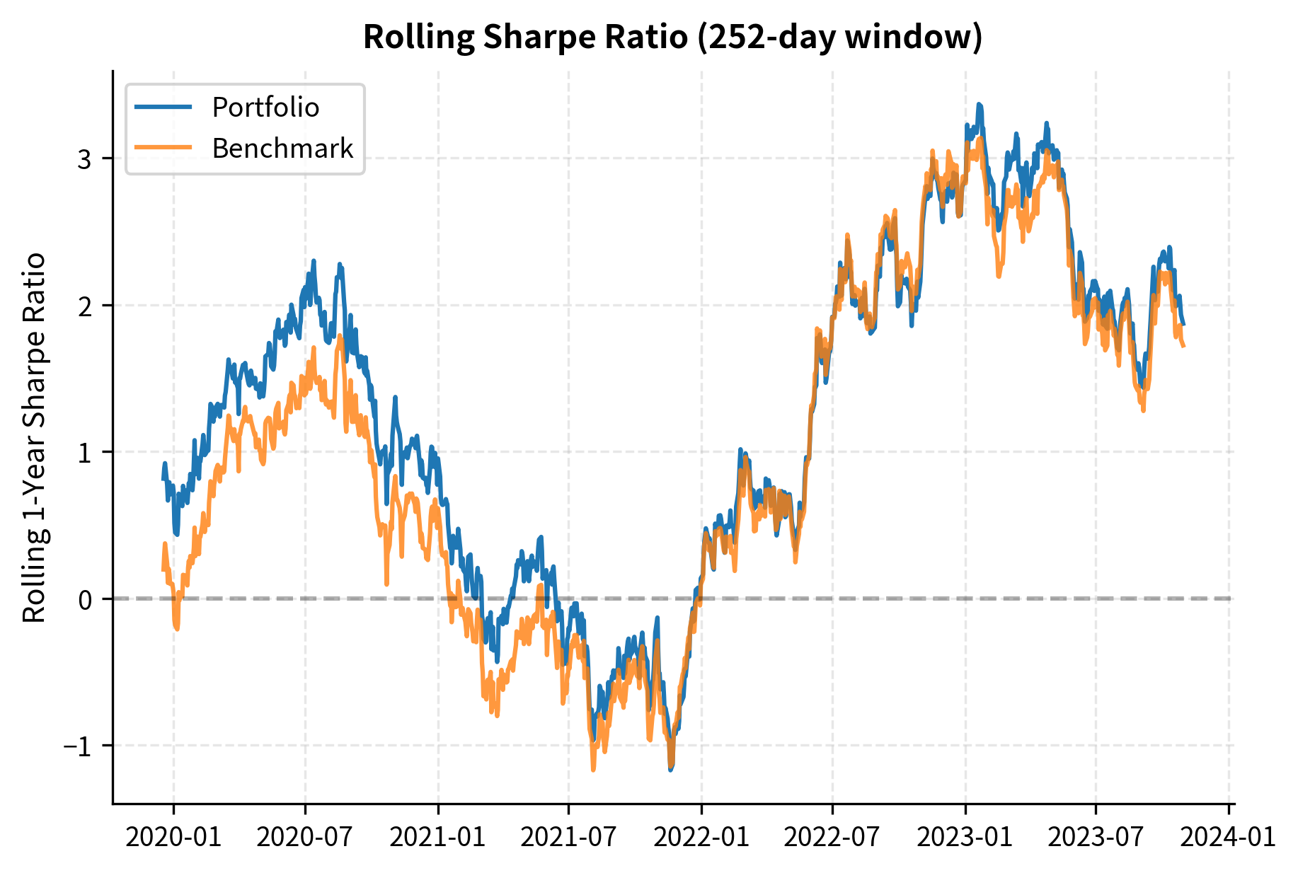
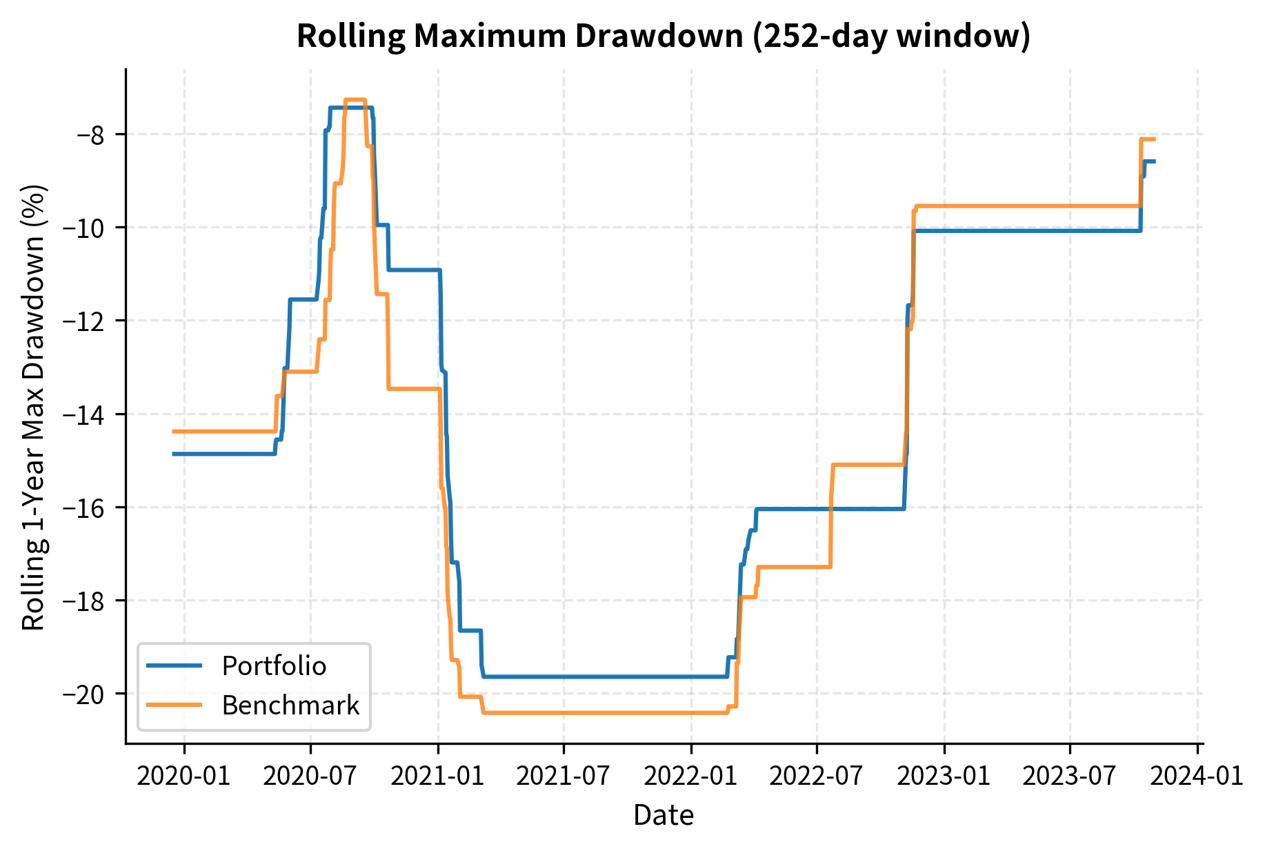
Rolling analysis reveals that performance metrics are not constants; they fluctuate with market conditions. A manager with an impressive full-period Sharpe ratio might have experienced extended periods of negative Sharpe, which rolling analysis would reveal.
Key Parameters
The key parameters used in the performance measurement code are:
- returns: Array or Series of periodic asset returns.
- benchmark_returns: Returns of the benchmark index for relative performance comparison.
- risk_free_rate: The return on a risk-free asset (e.g., T-bills) used to calculate excess returns.
- mar: Minimum Acceptable Return, the threshold used in the Sortino ratio calculation.
- periods_per_year: Annualization factor (), typically 252 for daily data or 12 for monthly data.
- window: The lookback period (number of observations) for rolling window analysis.
Limitations and Practical Considerations
Understanding the limitations of performance metrics is as important as computing them correctly. Each metric makes implicit assumptions that may not hold in practice.
Sharpe Ratio Limitations
The Sharpe ratio assumes returns are normally distributed, which conflicts with the stylized facts we discussed earlier in the book. Financial returns exhibit fat tails, skewness, and time-varying volatility, all of which the Sharpe ratio ignores. A strategy that earns steady small gains but occasionally suffers catastrophic losses (like selling volatility) can have an attractive Sharpe ratio despite its unappealing risk profile.
Furthermore, the Sharpe ratio is sensitive to the measurement period and frequency. The same strategy can have different Sharpe ratios when measured daily versus monthly, not just because of annualization differences, but because autocorrelation in returns affects how returns aggregate. Strategies with positive autocorrelation (momentum) will have higher Sharpe ratios at longer frequencies, while mean-reverting strategies show the opposite pattern.
The choice of risk-free rate also matters more than practitioners often acknowledge. During periods of near-zero interest rates, this seems trivial, but historically and in certain currencies, the risk-free rate significantly affects computed Sharpe ratios.
Information Ratio Limitations
The information ratio inherits the Sharpe ratio's assumption issues and adds benchmark selection risk. Choosing an inappropriate benchmark can make a mediocre manager look skilled or a skilled manager look mediocre. A small-cap value manager benchmarked against the S&P 500 will generate tracking error simply from style differences, not from active decisions.
The information ratio also assumes that alpha and tracking error are stable over time, which is rarely true. Managers may take more active risk in certain market conditions or when they have higher conviction. Averaging across these varying regimes can produce misleading summary statistics.
Maximum Drawdown Limitations
Maximum drawdown is inherently sample-dependent. It measures the worst observed outcome, but future drawdowns could be worse. The longer the track record, the larger the expected maximum drawdown, simply because more opportunities for drawdowns have occurred. Comparing maximum drawdowns across managers with different track record lengths is problematic.
Maximum drawdown is also highly path-dependent and sensitive to the specific sequence of returns. Two managers with identical return distributions but different timing will have different maximum drawdowns. This can make the metric feel arbitrary when a manager's maximum drawdown occurred due to a one-time market event rather than systemic strategy weaknesses.
Survivorship and Look-Ahead Bias
When evaluating historical performance, survivorship bias can inflate apparent results. Failed funds are not included in historical databases, making the average surviving fund look better than a randomly selected fund at inception would have been. Similarly, look-ahead bias occurs when performance measurement uses information that was not available at the time decisions were made. Using in-sample optimized weights to compute backtested Sharpe ratios produces overly optimistic results.
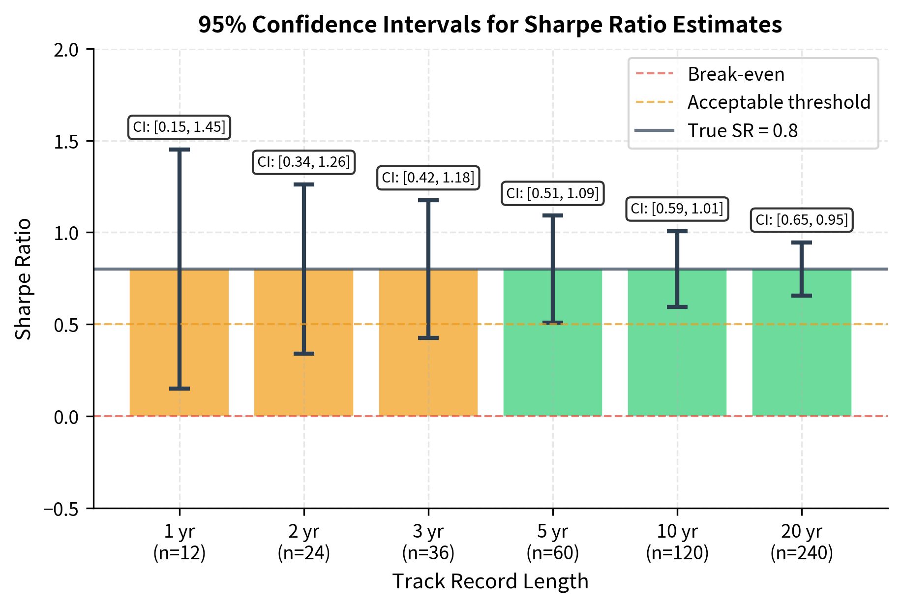
Statistical Significance
All computed metrics are estimates subject to sampling error. A Sharpe ratio of 0.8 based on three years of monthly data has substantial uncertainty around it. The standard error of the Sharpe ratio estimator is approximately:
where:
- : estimated Sharpe ratio
- : true Sharpe ratio
- : number of observations
The term inside the square root accounts for uncertainty in estimating both the mean (the ) and the variance (the ). For monthly data over three years () with a true Sharpe ratio of 0.8, the standard error is roughly 0.18, meaning a 95% confidence interval spans from about 0.44 to 1.16. This wide range highlights how difficult it is to distinguish skill from luck with limited data.
The same caution applies to the information ratio. A positive IR based on limited data may simply reflect sampling variation rather than genuine skill. Statistical tests for the significance of alpha, which we'll cover in the Performance Attribution chapter, help address this uncertainty.
Summary
This chapter developed the essential toolkit for evaluating portfolio performance beyond raw returns. The key metrics and their applications include:
Absolute risk-adjusted measures:
- The Sharpe ratio normalizes excess returns by volatility, enabling comparison across portfolios with different risk levels
- The Sortino ratio focuses on downside risk, making it appropriate for asymmetric return distributions
Relative performance measures:
- Active return and tracking error quantify how a portfolio differs from its benchmark
- The information ratio measures the efficiency of active management by relating alpha to active risk
Path-dependent risk measures:
- Maximum Drawdown captures the worst peak-to-trough decline, revealing tail risks that volatility misses
- The Calmar ratio relates returns to this worst-case scenario, penalizing strategies with catastrophic losses
Each metric illuminates a different aspect of performance, and no single number tells the complete story. Skilled performance evaluation requires examining multiple metrics together, understanding their limitations, and considering the statistical uncertainty inherent in finite samples.
In the next chapter on Performance Attribution, we'll decompose portfolio returns into their sources: how much came from market exposure, sector allocation, security selection, and timing. This analysis connects the performance metrics developed here to the underlying investment decisions that generated them.
Quiz
Ready to test your understanding? Take this quick quiz to reinforce what you've learned about portfolio performance measurement.

Comments