

Learn Arbitrage Pricing Theory and multi-factor models. Master Fama-French factors, estimate factor loadings via regression, and decompose portfolio risk.
Choose your expertise level to adjust how many terms are explained. Beginners see more tooltips, experts see fewer to maintain reading flow. Hover over underlined terms for instant definitions.
Arbitrage Pricing Theory and Multi-Factor Models
In the previous chapter, we explored the Capital Asset Pricing Model, which elegantly explains expected returns through a single factor: the market portfolio. While CAPM provides powerful insights, it relies on strong assumptions and reduces all systematic risk to one dimension. Real markets, however, are influenced by multiple sources of risk: interest rate changes, inflation surprises, oil price shocks, and shifts in investor sentiment toward different types of stocks.
Arbitrage Pricing Theory (APT), developed by Stephen Ross in 1976, offers a more flexible framework. Rather than prescribing a single source of systematic risk, APT allows for multiple factors to drive returns. The theory rests on a simple but powerful idea: in well-functioning markets, arbitrage opportunities cannot persist. This no-arbitrage condition, combined with a factor structure for returns, yields pricing relationships similar to CAPM but with greater generality.
This chapter develops the APT framework from first principles, then explores its practical implementation through multi-factor models. We'll examine the famous Fama-French factors that have transformed empirical finance, learn to estimate factor exposures through regression, and build working factor models. By the end, you'll understand both the theoretical foundations and practical applications of factor-based investing.
The Limitations of Single-Factor Models
Before diving into APT, let's understand why we need something beyond CAPM. The single-factor model assumes that the market portfolio captures all systematic risk. Under this view, two stocks with the same beta should have identical expected returns, regardless of their other characteristics.
Empirical evidence tells a different story. Decades of research have documented persistent patterns that CAPM cannot explain:
- Size effect: Small-capitalization stocks have historically outperformed large-cap stocks, even after adjusting for their higher market betas
- Value premium: Stocks with high book-to-market ratios (value stocks) have earned higher returns than growth stocks with similar betas
- Momentum: Stocks that performed well over the past year tend to continue outperforming in the near term
- Profitability: More profitable firms earn higher returns than predicted by their market exposure alone
These anomalies suggest multiple sources of risk affect returns. A multi-factor framework better describes reality and provides more accurate risk assessment.
The APT Framework
This section develops the theoretical foundations of APT, starting with its factor structure assumptions and building toward the pricing equation that emerges from no-arbitrage conditions.
Assumptions and Factor Structure
APT begins with a fundamental assumption about how asset returns are generated. The core insight is that returns do not arise in isolation. Instead, they emerge from a combination of economy-wide forces that affect many assets simultaneously, plus company-specific events that affect only individual securities. This leads naturally to a linear factor model structure.
Each asset's return follows a linear factor model:
where:
- : The realized return on asset
- : The expected return on asset
- : The -th factor, representing a common source of risk. These are zero-mean surprise terms:
- : The sensitivity of asset to factor , often called the factor loading or factor beta
- : The idiosyncratic return component, specific to asset . By assumption, and for
To understand this equation intuitively, think of it as a decomposition of returns into three distinct components. First, there is the expected return, which represents the baseline compensation investors anticipate for holding the asset. Second, there are the factor-related components, which capture how the asset responds to various systematic shocks in the economy. Third, there is the idiosyncratic term, which reflects news and events specific to that particular company.
The factors capture systematic risks that affect many assets simultaneously. When the Federal Reserve unexpectedly raises interest rates, this represents a realization of an interest rate factor that simultaneously affects bank stocks, utility stocks, and bond prices. When oil prices spike unexpectedly, energy companies and airlines experience common shocks through an oil price factor. The key insight is that these systematic factors create correlations across assets, linking the fortunes of securities that might otherwise seem unrelated.
The idiosyncratic term represents asset-specific news: earnings surprises, management changes, or product announcements that affect only that particular asset. A pharmaceutical company receiving FDA approval for a new drug experiences an idiosyncratic shock. This news affects that company's stock but has no direct impact on an unrelated technology firm. The assumption that idiosyncratic terms are uncorrelated across assets is crucial because it means that holding many assets allows investors to diversify away this company-specific risk.
A subtle but important distinction: the factors in the return equation are surprise components (deviations from expected values), not the factor values themselves. If inflation was expected to be 3% but realized at 4%, the inflation factor equals 1%, not 4%.
APT requires relatively mild assumptions compared to CAPM:
- Returns follow the factor structure described above
- There are enough assets to diversify away idiosyncratic risk
- Markets are competitive, and investors prefer more wealth to less
- No arbitrage opportunities exist
Notice what's absent: APT does not require investors to have identical expectations, does not assume all investors hold the market portfolio, and does not require returns to be normally distributed. This generality comes at a cost: APT does not tell us what the factors are or how many exist.
The No-Arbitrage Argument
The pricing relationship in APT emerges from the absence of arbitrage. This is a powerful approach because it requires only that markets function well enough to prevent riskless profit opportunities, rather than requiring that all investors behave optimally or hold identical beliefs.
Consider a well-diversified portfolio where idiosyncratic risk has been eliminated. When a portfolio contains many securities with independent idiosyncratic components, the law of large numbers ensures that these random shocks largely cancel out. The positive surprises from some holdings offset the negative surprises from others. In the limit, as the number of holdings grows large, idiosyncratic risk effectively vanishes.
Such a portfolio's return depends only on its factor exposures:
where:
- : return on the portfolio
- : expected return on the portfolio
- : sensitivity of the portfolio to factor
- : factor
This equation reveals something profound. Once idiosyncratic risk is diversified away, the portfolio's realized return differs from its expected return only because of factor surprises. If you could somehow construct a portfolio with zero exposure to all factors, you would know its return with certainty before it occurred.
Now consider constructing a portfolio with zero exposure to all factors, achieved by appropriate weighting of assets. This zero-factor portfolio bears no systematic risk. In the absence of arbitrage, it must earn the risk-free rate:
where:
- : expected return on the portfolio
- : risk-free rate
- : sensitivity of the portfolio to factor
The logic here is compelling. If such a portfolio earned more than the risk-free rate, investors could borrow at the risk-free rate, invest in the portfolio, and earn a guaranteed profit with no risk. This would be a pure arbitrage opportunity. Conversely, if the portfolio earned less than the risk-free rate, investors could short the portfolio, invest the proceeds at the risk-free rate, and again earn a guaranteed profit. Competition among arbitrageurs ensures that neither situation can persist, forcing the zero-factor portfolio to earn exactly the risk-free rate.
Similarly, two portfolios with identical factor exposures must have identical expected returns. Otherwise, you could go long the higher-return portfolio, short the lower-return portfolio, and earn a risk-free profit.
The APT Pricing Equation
These no-arbitrage conditions imply a linear relationship between expected returns and factor exposures:
where:
- : expected return on asset
- : risk-free rate
- : sensitivity of asset to factor
- : risk premium for factor , representing the additional expected return earned per unit of exposure to that factor
This is the central result of APT. The equation states that expected returns are determined entirely by factor exposures. An asset's expected return equals the risk-free rate plus compensation for each unit of systematic risk borne. The lambda terms represent the market price of each type of risk. If factor carries a risk premium of 4%, then an asset with a factor loading of 1.5 on that factor earns an additional 6% (1.5 times 4%) in expected return.
To derive this more formally, consider portfolios: one with zero exposure to all factors, and portfolios each with unit exposure to exactly one factor. The zero-exposure portfolio earns . A portfolio with unit exposure to factor and zero exposure to all other factors earns .
For any asset or portfolio with arbitrary factor exposures , you can replicate its factor risk using combinations of these basis portfolios. Think of it as building a synthetic version of the asset using building blocks of pure factor exposure. The no-arbitrage condition requires the asset's expected return to equal the replicating portfolio's return, giving us the APT pricing equation.
The derivation is simple and requires no assumptions about investor preferences, wealth distributions, or equilibrium conditions. The mere requirement that arbitrage opportunities be absent, combined with the factor structure of returns, delivers a complete pricing relationship.
Comparing APT and CAPM
The APT pricing equation resembles CAPM but with crucial differences:
| Aspect | CAPM | APT |
|---|---|---|
| Number of factors | Single (market) | Multiple (unspecified) |
| Factor identification | Prescribed (market portfolio) | Not specified |
| Theoretical basis | Equilibrium with utility maximization | No-arbitrage |
| Assumptions | Strong (normal returns, homogeneous expectations) | Weak (factor structure, no arbitrage) |
| Testability | Requires identifying the true market portfolio | Requires identifying the relevant factors |
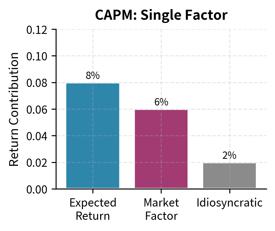
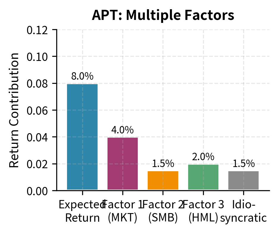
CAPM is actually a special case of APT when there is only one factor and that factor is the market return. In this case, (the market risk premium), and we recover the familiar CAPM equation.
These models illustrate a broader principle in financial economics: APT gains generality through weaker assumptions but offers less specific predictions. CAPM tells us exactly which factor matters, namely the market portfolio, but requires strong assumptions that may not hold in practice. APT allows for multiple factors and requires only no-arbitrage, but it does not tell us which factors are relevant or how many to include. This trade-off between generality and specificity recurs throughout finance theory.
Multi-Factor Models in Practice
APT provides a theoretical foundation but leaves the factors unspecified. In practice, researchers and practitioners have developed two main approaches to identifying factors: macroeconomic factor models and fundamental factor models.
Macroeconomic Factor Models
Macroeconomic models use observable economic variables as factors. This approach is intuitive: since factors represent systematic risks that affect many assets, they should correspond to economy-wide variables that influence corporate profits, discount rates, and investor behavior.
Chen, Roll, and Ross (1986) proposed a five-factor model using:
- Industrial production growth: Captures the state of the real economy
- Changes in expected inflation: Affects discount rates and corporate profits differently
- Unexpected inflation: Transfers wealth between borrowers and lenders
- Credit spread changes: The difference between corporate and government bond yields, capturing default risk perceptions
- Term structure changes: Shifts in the yield curve slope, affecting the relative pricing of different maturities
Each of these variables has clear economic content. Industrial production growth measures the real output of the economy, and stocks of companies with greater exposure to economic cycles should be more sensitive to this factor. Unexpected inflation redistributes wealth between debtors and creditors, benefiting firms with fixed-rate debt while harming those with fixed-rate assets. Credit spread changes signal shifts in the perceived riskiness of corporate debt, which naturally affects equity values as well.
Macroeconomic factors offer clear economic interpretations, but data lags and revisions make real-time implementation challenging.
Fundamental Factor Models
Fundamental factor models use characteristics of securities themselves to explain returns. Rather than specifying macroeconomic variables, these models identify factors based on firm attributes that have historically explained return differences.
This approach differs from macroeconomic models by asking which characteristics have predicted returns historically rather than specifying which economic variables should affect returns. This empirical focus reveals patterns not obvious from economic reasoning.
The most influential fundamental factor model is the Fama-French framework, which we examine in detail next.
The Fama-French Factor Models
Eugene Fama and Kenneth French revolutionized empirical asset pricing with their 1993 three-factor model, later extended to five factors in 2015. These models have become the standard benchmark for evaluating investment performance and understanding return patterns.
The Three-Factor Model
The Fama-French three-factor model augments CAPM with two additional factors:
where:
- : return on asset
- : risk-free rate
- : intercept (abnormal return)
- : sensitivities to the respective factors
- : market factor ()
- : size factor (Small Minus Big)
- : value factor (High Minus Low)
- : idiosyncratic error term
The model's structure reveals its purpose. The left-hand side measures the asset's excess return over the risk-free rate, which represents the premium investors earn for bearing risk. The right-hand side decomposes this premium into components: compensation for market risk, for size-related risk, for value-related risk, and any residual alpha that the factors cannot explain.
The factors are defined as follows:
-
MKT (Market): The excess return on a broad market portfolio, identical to the CAPM market factor.
-
SMB (Small Minus Big): The return on a portfolio of small-cap stocks minus the return on a portfolio of large-cap stocks. SMB captures the size premium: small stocks' tendency to outperform large stocks
-
HML (High Minus Low): The return on a portfolio of high book-to-market (value) stocks minus the return on a portfolio of low book-to-market (growth) stocks. HML captures the value premium
The construction of SMB and HML as long-short portfolios is deliberate. By going long small stocks and short large stocks, SMB isolates the pure effect of size, controlling for other characteristics. Similarly, by going long value stocks and short growth stocks, HML isolates the pure effect of valuation. This long-short construction ensures that the factors are approximately uncorrelated with the market factor, making them useful for explaining return variation beyond what CAPM captures.
SMB and HML are not tradeable assets but portfolios constructed specifically to isolate size and value exposures. Fama and French construct these by sorting stocks into groups based on size and book-to-market, then taking appropriate long-short combinations.
Constructing the SMB and HML Factors
The construction methodology matters for understanding what these factors capture. Each year at the end of June, Fama and French sort stocks as follows:
Size sort: Stocks are ranked by market capitalization and divided at the median into Small and Big groups.
Book-to-market sort: Stocks are independently ranked by book-to-market ratio and divided into three groups: Low (bottom 30%), Medium (middle 40%), and High (top 30%).
This creates six portfolios from the intersection of two size groups and three book-to-market groups. The factors are then computed as:
where:
- : portfolio of small-cap, high book-to-market stocks
- : portfolio of large-cap, high book-to-market stocks
- : portfolio of small-cap, medium book-to-market stocks
- : portfolio of large-cap, medium book-to-market stocks
- : portfolio of small-cap, low book-to-market stocks
- : portfolio of large-cap, low book-to-market stocks
The averaging process in these formulas serves an important purpose. The SMB factor averages across book-to-market groups, isolating the size effect. By including small value, small medium, and small growth stocks on the long side, and big value, big medium, and big growth stocks on the short side, the factor captures the pure size effect without being contaminated by any particular book-to-market exposure.
The HML factor averages across size groups, isolating the value effect. By including both small and big value stocks on the long side, and both small and big growth stocks on the short side, the factor captures the pure value effect without being contaminated by size effects.
The Five-Factor Model
In 2015, Fama and French extended their model with two additional factors based on profitability and investment:
where:
- : defined as in the three-factor model
- : sensitivity to factor
- : market, size, and value factors
- : profitability factor (Robust Minus Weak)
- : investment factor (Conservative Minus Aggressive)
Empirical observation and theoretical reasoning motivated adding these factors. Empirically, researchers found that profitability and investment patterns explained return variation not captured by the original three factors. Theoretically, these factors connect to fundamental valuation principles.
The new factors are:
-
RMW (Robust Minus Weak): The return on stocks with robust (high) operating profitability minus stocks with weak (low) profitability. Companies with higher profit margins tend to earn higher returns
-
CMA (Conservative Minus Aggressive): The return on stocks of companies with conservative (low) investment minus aggressive (high) investment. Firms that invest less tend to earn higher returns
The profitability factor has intuitive appeal. All else equal, a more profitable company should be worth more. If two companies have similar market prices but different profitabilities, the more profitable one offers better value and should earn higher subsequent returns. The investment factor relates to the rate at which companies are expanding their asset base. Firms investing heavily may be pursuing growth at the expense of current profitability, or they may be making poor capital allocation decisions. Either interpretation suggests that conservative investors, those who invest less aggressively, may earn higher returns.
The Momentum Factor
While not part of the original Fama-French framework, momentum has become a standard factor in many models. The momentum factor (often called UMD for "Up Minus Down" or WML for "Winners Minus Losers") captures the tendency of recent winners to continue outperforming:
where:
- : return on the portfolio of recent top-performing stocks
- : return on the portfolio of recent bottom-performing stocks
Stocks are sorted based on their past 12-month returns (excluding the most recent month to avoid microstructure effects), and the factor is the return difference between the top and bottom deciles.
The exclusion of the most recent month is a subtle but important detail. Stock prices exhibit short-term reversal at very short horizons due to microstructure effects like bid-ask bounce. By skipping the most recent month, the momentum factor captures medium-term continuation rather than short-term noise.
Mark Carhart's 1997 four-factor model combined the Fama-French three factors with momentum:
where:
- : return on asset
- : risk-free rate
- : intercept (abnormal return)
- : idiosyncratic error term
- : Fama-French three factors
- : Momentum factor
- : sensitivity to factor
This model has become particularly popular for evaluating mutual fund performance. By including momentum, the model can distinguish between managers who generate alpha through stock selection and those who simply ride momentum trends.
Estimating Factor Exposures
With the factor model framework established, we now turn to the practical task of estimating an asset's factor exposures. As we discussed in Part III's chapter on Regression Analysis, time-series regression provides a natural estimation approach.
Time-Series Regression
For an individual stock or portfolio, we regress excess returns on the factor returns:
where:
- : excess return on asset at time
- : estimated alpha
- : estimated factor loadings
- : factor return at time
- : residual at time
This regression has a natural interpretation. The dependent variable, excess return, is what we seek to explain. The independent variables, the factor returns, represent the systematic risk sources. The regression coefficients tell us how much the asset's return moves, on average, in response to each factor.
The regression coefficients , , and are the estimated factor loadings. The intercept represents the average return not explained by the factors: positive alpha suggests outperformance, negative alpha suggests underperformance.
The interpretation of factor loadings is straightforward:
- : The asset behaves like a small-cap stock
- : The asset behaves like a large-cap stock
- : The asset behaves like a value stock
- : The asset behaves like a growth stock
These interpretations connect statistical estimates to economic meaning. A stock with a large positive SMB loading tends to rise when small stocks outperform large stocks, regardless of the company's actual market capitalization. The factor loading captures behavioral similarity rather than category membership.
Cross-Sectional Regression
An alternative approach estimates factor risk premia rather than individual factor loadings. In cross-sectional regression, we use known or estimated betas as explanatory variables and current returns as the dependent variable:
where:
- : return on asset at time
- : intercept (zero-beta rate) at time
- : estimated risk premium for the factor at time
- : estimated factor loading for asset (from first pass)
- : pricing error
This regression is run across all assets at each point in time, yielding time series of estimated risk premia . The average of these estimates gives the historical factor risk premium.
The logic of cross-sectional regression differs fundamentally from time-series regression. In time-series regression, we ask: "Given that we know what the factors did, how sensitive was this particular asset?" In cross-sectional regression, we ask: "Given that we know each asset's sensitivities, what premium did the market pay for each type of risk?"
The Fama-MacBeth procedure (1973) formalizes this two-step approach:
- First pass: Time-series regressions to estimate each asset's factor betas
- Second pass: Cross-sectional regressions at each date to estimate factor premia
This methodology remains the standard for testing factor pricing models. It provides not only point estimates of factor premia but also standard errors that account for the time-series variation in estimated premia.
Working with Factor Data
Let's implement a factor model using real data. The Fama-French factors are publicly available from Kenneth French's data library. We'll use the pandas-datareader library to access this data directly.
The data contains monthly returns for each factor plus the risk-free rate. Let's examine the historical factor premia.
The Sharpe ratios indicate risk-adjusted performance. A higher Sharpe ratio suggests better compensation for each unit of risk taken.
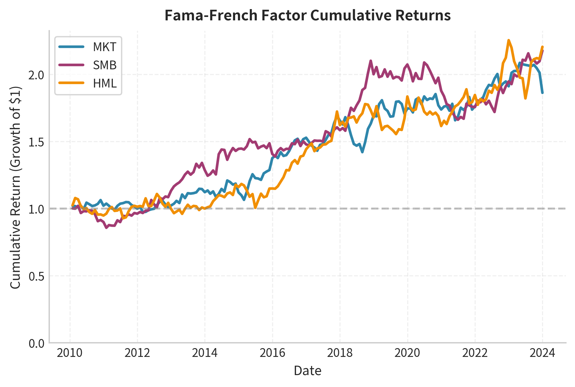
Visualizing Factor Returns
Let's visualize the cumulative performance of each factor.
The chart reveals important patterns in factor performance. The market factor (MKT) showed strong positive returns over this period, reflecting the bull market in U.S. equities. The SMB factor exhibited weaker performance, as large-cap stocks dominated returns in many years. The HML factor actually produced negative returns over much of this period, as growth stocks significantly outperformed value stocks.
These patterns highlight an important caveat: factor premia are not guaranteed. While historical data shows positive average returns to size and value over long periods, individual decades can show very different patterns.
Factor Correlations
Understanding factor correlations helps with portfolio construction and risk management.
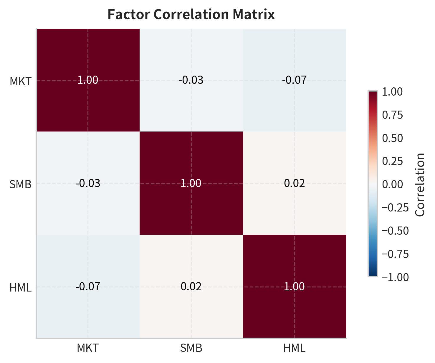
The relatively low correlations between factors confirm that they capture distinct sources of systematic risk. This makes multi-factor models valuable for both explaining returns and constructing diversified portfolios.
Estimating Factor Loadings for a Stock
Now let's estimate factor loadings for a specific stock. We'll create synthetic return data that mimics a real stock's behavior, then estimate its factor exposures using regression.
The regression successfully recovers the true factor loadings. The R-squared indicates what fraction of return variance is explained by the factors. The remaining variance represents idiosyncratic risk that could be diversified away in a portfolio.
Interpreting the Results
Let's compare our estimates to the true values and interpret the stock's factor profile.
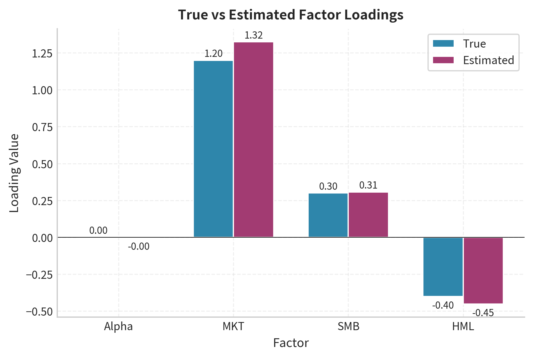
The estimated loadings closely match the true values. The small differences arise from estimation error due to finite sample size and idiosyncratic noise. This stock has:
- High market beta (1.2): More volatile than the market, amplifying gains in bull markets and losses in bear markets
- Positive SMB loading (0.3): Behaves somewhat like a small-cap stock, gaining when small stocks outperform
- Negative HML loading (-0.4): Behaves like a growth stock, gaining when growth outperforms value
This profile is typical of a technology growth stock: high market sensitivity, modest small-cap characteristics, and strong growth orientation.
Building a Multi-Factor Risk Model
Factor models serve two purposes: explaining expected returns and decomposing risk. Let's build a complete factor risk model for a portfolio.
Portfolio Factor Exposures
For a portfolio with weights across assets, the portfolio's factor exposure is the weighted average of individual exposures:
where:
- : portfolio sensitivity to factor
- : weight of asset in the portfolio
- : sensitivity of asset to factor
- : number of assets
This linearity makes factor models computationally tractable for large portfolios. Rather than tracking the correlations among thousands of individual securities, we need only track each security's exposure to a handful of factors. The portfolio's risk characteristics are then determined by its aggregate factor exposures, a dramatic simplification that enables practical risk management for institutional portfolios.
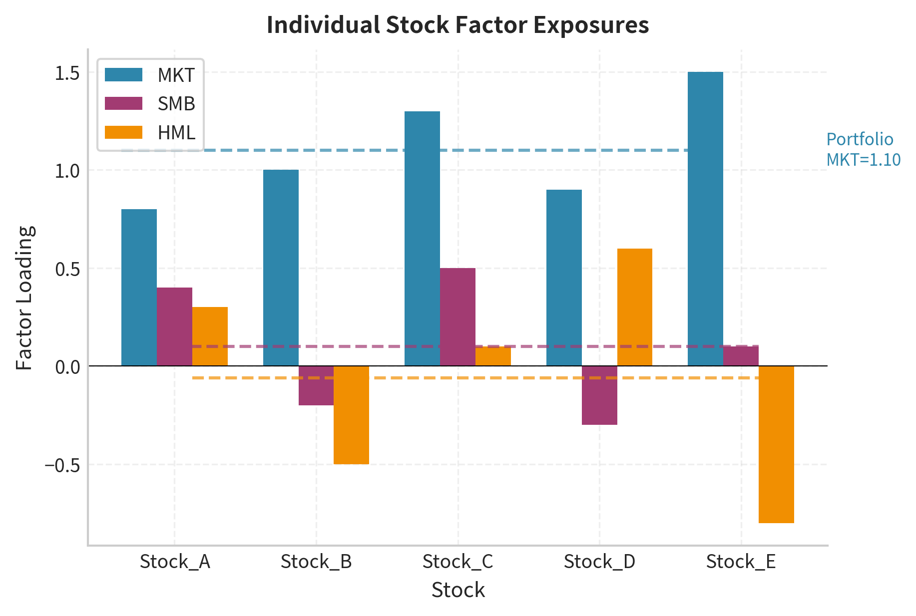
The portfolio maintains a market beta near 1.0 but has specific net exposures to size and value factors based on the underlying holdings.
Factor Risk Decomposition
The total variance of a portfolio in a factor model decomposes into factor risk and idiosyncratic risk. This decomposition is one of the most powerful applications of factor models because it separates diversifiable risk from non-diversifiable risk.
Using the factor covariance matrix and idiosyncratic variances :
where:
- : portfolio variance
- : vector of portfolio factor exposures
- : covariance matrix of factor returns
- : weight of asset
- : idiosyncratic variance of asset
The first term is systematic risk from factor exposures. This term depends on how the factors co-move with each other and how much exposure the portfolio has to each factor. Even with perfect diversification across many securities, this systematic risk cannot be eliminated because it arises from economy-wide forces.
The second term is idiosyncratic risk, which decreases as the portfolio becomes more diversified. Notice that individual idiosyncratic variances are multiplied by squared weights. When weights are small (as in a well-diversified portfolio), squared weights become very small, causing the idiosyncratic component to shrink rapidly.
The diagonal elements represent the variance of each factor, while off-diagonal elements show co-movements. Low off-diagonal values confirm the factors provide diversification benefits.
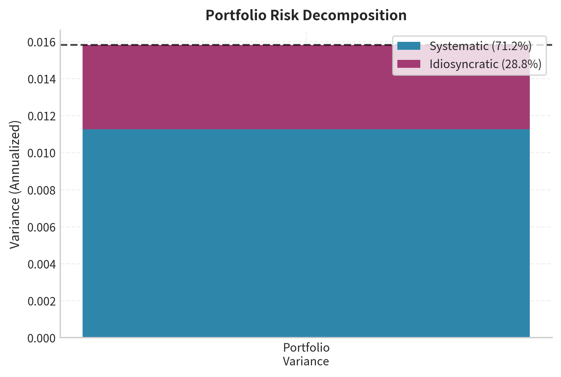
The decomposition shows that systematic factor risk dominates, accounting for most of the portfolio variance. The idiosyncratic component is small because diversification across five stocks reduces stock-specific risk. With more holdings, idiosyncratic risk would decrease further.
Marginal Contribution to Risk
Understanding which positions contribute most to portfolio risk helps with risk management. The marginal contribution to risk (MCTR) measures how much total volatility would change with a small increase in each position's weight:
where:
- : marginal contribution to risk of asset
- : portfolio volatility
- : weight of asset
- : return on asset
- : return on the portfolio
Intuitively, the MCTR shows that an asset's contribution to risk depends not on its standalone volatility, but on its covariance with the portfolio. Assets that move in sync with the portfolio increase risk, while those that move inversely can reduce it.
This insight has profound implications for portfolio construction. A highly volatile stock that is negatively correlated with the rest of the portfolio might actually reduce total portfolio risk when added. Conversely, a low-volatility stock that is highly correlated with existing holdings might substantially increase risk. The MCTR captures these portfolio-level effects that are invisible when examining securities in isolation.
Stock E, with its high market beta and growth tilt, contributes disproportionately to risk despite having equal weight. This analysis helps identify risk concentrations and informs rebalancing decisions.
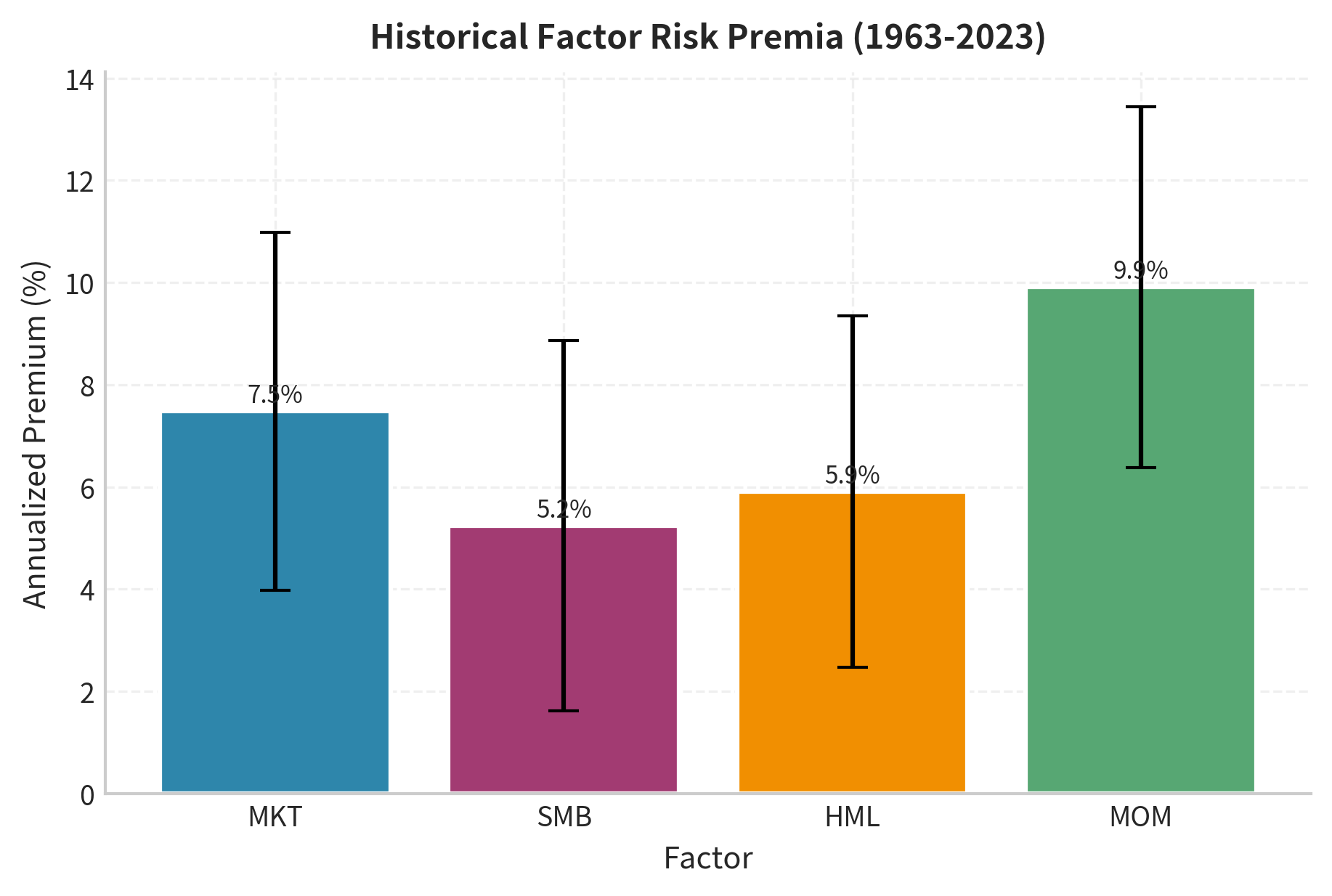
Factor Risk Premia: Evidence and Interpretation
A central question in factor investing is whether factor exposures are compensated with higher expected returns. Let's examine the historical evidence for factor risk premia.
All four factors show positive average returns over the full sample. The t-statistics help assess statistical significance: values above 2.0 suggest the premium is unlikely due to chance. The market premium is highly significant, as expected. SMB and HML show meaningful premia, though with lower significance than the market. Momentum displays a strong premium with high statistical significance.
Rolling Factor Performance
Factor premia are not constant over time. Let's examine how factor performance has varied across different periods.
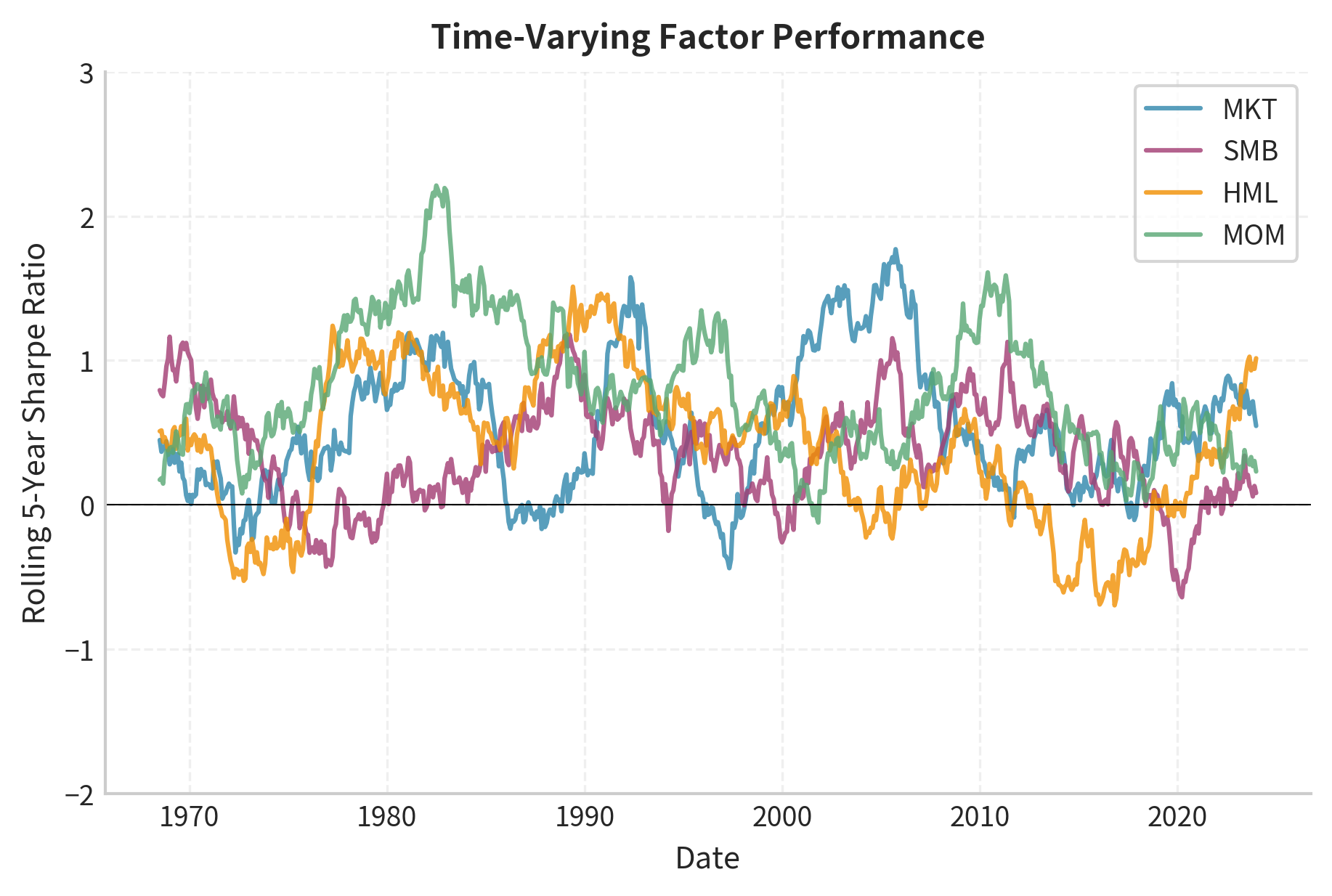
The rolling analysis reveals substantial time variation in factor performance. Some observations:
- The market factor shows persistent positive Sharpe ratios but with significant variation
- SMB performance was strong in the 1970s-1980s but weakened substantially after 2000
- HML showed strong performance through the 1990s but turned negative in the 2010s
- Momentum displays high volatility, with occasional sharp negative drawdowns (notably 2009)
This time variation raises important questions: Do factor premia persist because they compensate for risk, or were historical patterns data-mined anomalies that have since been arbitraged away?
Economic Interpretations of Factor Premia
Several theories attempt to explain why factor premia exist. Understanding these theories helps practitioners form views about whether premia will persist in the future.
Risk-based explanations argue that factors proxy for systematic risks. Small stocks may earn higher returns because they are more vulnerable to economic downturns. When the economy contracts, small firms often lack the financial resources, customer diversification, and market power to weather the storm. Investors who hold small stocks bear this recession risk and demand higher expected returns as compensation. Value stocks may be riskier because they often represent distressed firms or those facing structural challenges. A company with a high book-to-market ratio may be cheap because investors doubt its future prospects. Holding such companies exposes investors to the risk that these doubts prove justified.
Behavioral explanations suggest factors arise from investor biases. Investors may overpay for glamorous growth stocks, creating the value premium. The allure of companies with exciting products and rapid growth may cause investors to extrapolate past success too far into the future, bidding prices above fundamental value. Momentum may reflect slow information diffusion or herding behavior. When good news emerges, it may take time for all investors to learn and process the information, causing prices to adjust gradually rather than instantaneously.
Limits to arbitrage explanations note that even if mispricings exist, arbitraging them is costly and risky. Short-selling constraints, career risk for fund managers, and factor crash risk may prevent full correction of factor-related mispricings. A fund manager who shorts overvalued growth stocks might be correct in the long run but could face client redemptions if the strategy underperforms in the short run. This career risk limits the capital that flows to correct mispricings.
The debate continues, but the practical implication is clear: factor exposures matter for understanding portfolio risk, regardless of whether the premia persist.
Multi-Factor Model Applications
Factor models serve multiple purposes in quantitative finance. Let's explore some key applications.
Performance Attribution
When evaluating a portfolio manager's performance, factor models separate skill (alpha) from systematic risk exposures (factor returns). A manager who outperformed the market may have done so simply by taking more factor risk rather than through superior stock selection.
This distinction matters enormously for investors deciding whether to pay active management fees. If a manager's outperformance comes entirely from factor tilts, investors could achieve similar results at lower cost by using passive factor-based strategies. True alpha, the return that cannot be explained by factor exposures, represents genuine skill or information advantage that may justify higher fees.
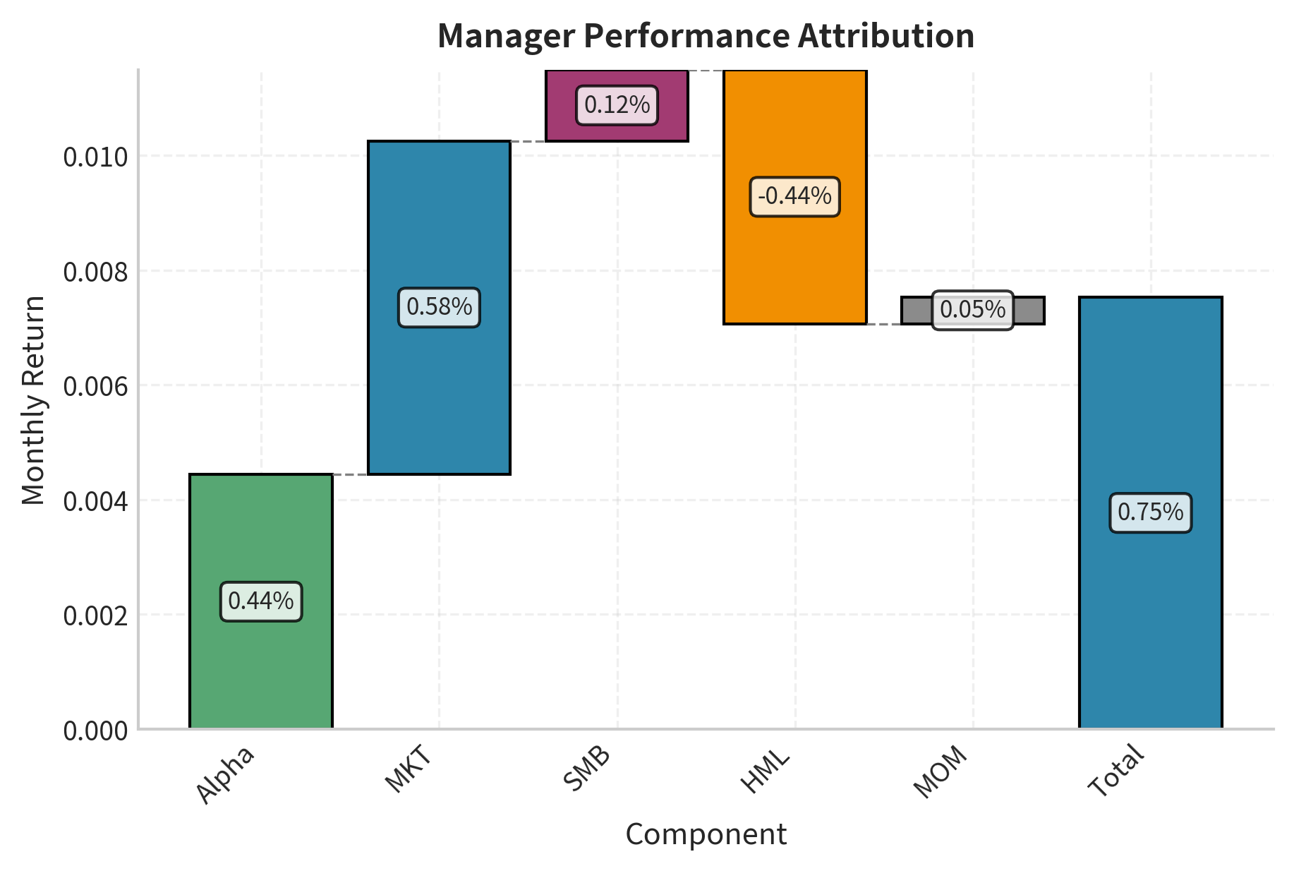
This decomposition shows how much of the manager's return came from factor tilts versus true stock selection skill. In this example, the market exposure contributes most to returns, followed by alpha.
Risk Budgeting
Factor models enable risk budgeting: allocating a portfolio's total risk across factors according to a target risk profile. This approach is increasingly used in institutional portfolio management.
The concept of risk budgeting treats risk as a scarce resource to be allocated deliberately. Just as a household budgets its income across different spending categories, an institutional investor budgets its risk tolerance across different risk sources. Factor models provide the framework for measuring and managing these risk allocations.
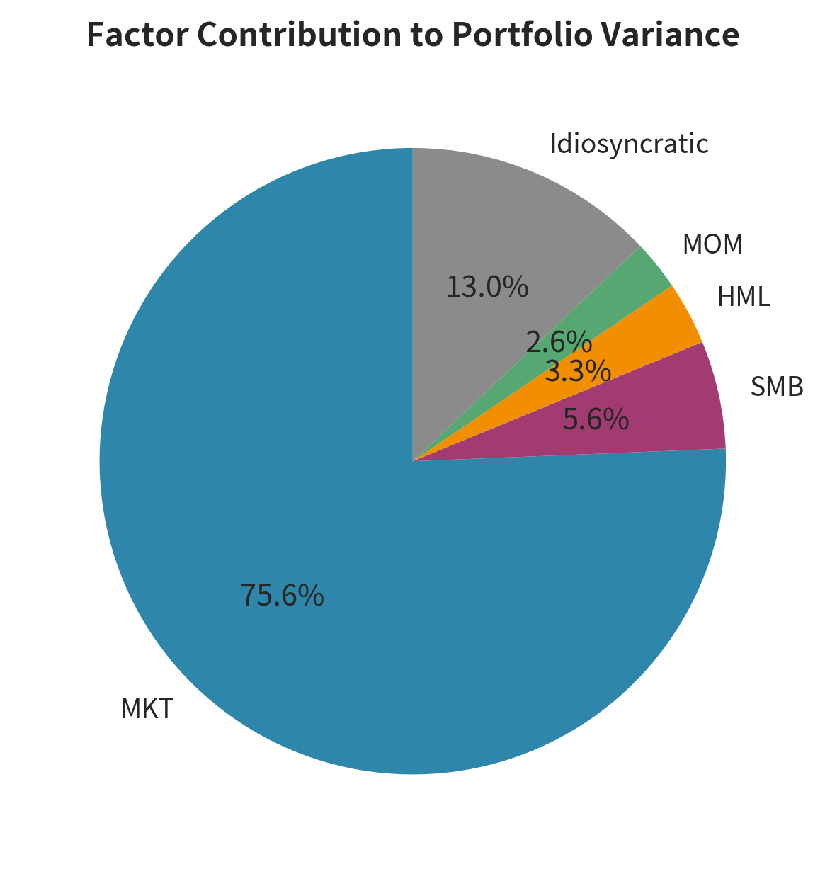
The chart illustrates the dominance of market risk in the portfolio. Despite holding five stocks with various factor tilts, the general market movement still accounts for the majority of the portfolio's volatility.
Factor-Based Portfolio Construction
Factor models also guide portfolio construction. A manager might target specific factor exposures while minimizing idiosyncratic risk:
This portfolio would match market risk (beta = 1.0), be size-neutral, tilt toward value stocks (positive HML), and be momentum-neutral.
Building such a portfolio requires optimizing stock weights subject to factor exposure constraints. We'll explore this further in the upcoming chapter on Advanced Portfolio Construction Techniques.
Key Parameters
The key parameters for the Multi-Factor Models discussed in this chapter are:
- MKT: Market factor return (). A proxy for broad equity market risk.
- SMB: Size factor return (Small Minus Big). The return difference between small-cap and large-cap stocks.
- HML: Value factor return (High Minus Low). The return difference between value (high B/M) and growth (low B/M) stocks.
- MOM: Momentum factor return (Up Minus Down). The return difference between recent winners and losers.
- : Factor loading. The sensitivity of asset to factor , estimated via time-series regression.
- : Factor risk premium. The expected excess return earned per unit of exposure to factor .
- : Alpha. The abnormal return of asset not explained by the factor exposures.
Limitations and Practical Considerations
The Factor Zoo Problem
Academic research has documented hundreds of factors that allegedly predict returns. Harvey, Liu, and Zhu (2016) found that researchers had tested over 300 factors, many of which are likely false positives. This "factor zoo" creates challenges:
- Data mining: With enough testing, random patterns appear significant
- Publication bias: Journals prefer significant results, so null findings go unreported
- Overfitting: Models with many factors may fit historical data but fail out-of-sample
Practitioners typically focus on factors with strong theoretical justification, robust evidence across time periods and markets, and economic magnitude sufficient to survive transaction costs.
Estimation Challenges
Factor loadings are estimated with error, and these errors can compound in portfolio optimization. Several issues arise:
- Time-varying betas: Factor exposures change as firms evolve, making historical estimates unreliable
- Multicollinearity: When factors are correlated, individual beta estimates become unstable
- Survivorship bias: Databases often exclude failed companies, biasing factor premium estimates
Robust estimation techniques, Bayesian shrinkage methods, and ensemble approaches help address these challenges.
Transaction Costs and Implementation
Factor strategies require periodic rebalancing as firm characteristics change. This creates turnover and transaction costs that can erode gross returns. The momentum factor is particularly affected because it requires frequent trading to maintain exposure to recent winners.
Factor timing, attempting to increase exposure to factors expected to perform well, adds another layer of complexity. While factor premia are somewhat predictable using valuation spreads and other signals, reliable timing remains elusive.
Model Risk
Factor models, like all models, are simplifications of reality. Using them requires acknowledging their limitations:
- Factors may not capture all sources of systematic risk
- The relationship between factors and returns may change over time
- Extreme events may not be well-described by normal factor distributions
As we'll explore in Part V on Risk Management, model risk is a form of operational risk that must be managed through model validation, stress testing, and skepticism about model outputs.
Summary
This chapter developed the Arbitrage Pricing Theory framework and its practical implementation through multi-factor models. The key concepts covered include:
APT provides a general equilibrium-free framework for asset pricing. By assuming a factor structure for returns and imposing no-arbitrage conditions, APT derives a linear relationship between expected returns and factor exposures without requiring CAPM's restrictive assumptions.
Multi-factor models explain returns through multiple systematic risk sources. The Fama-French factors (market, size, value, profitability, investment) and momentum have become standard tools for understanding return variation and evaluating performance.
Factor loadings are estimated through time-series regression. Regressing asset excess returns on factor returns yields estimates of systematic risk exposures and alpha. Cross-sectional regression provides estimates of factor risk premia.
Factor models enable risk decomposition and attribution. Total portfolio risk splits into systematic (factor) and idiosyncratic components. This decomposition supports risk budgeting, performance attribution, and portfolio construction.
Factor premia vary over time and may not persist. Historical evidence shows meaningful factor premia, but individual periods can differ dramatically from long-term averages. Whether premia reflect risk compensation, behavioral biases, or data mining remains debated.
The next chapter on Portfolio Performance Measurement will build on these concepts, showing how to evaluate investment returns after accounting for factor exposures and risk taken.
Quiz
Ready to test your understanding? Take this quick quiz to reinforce what you've learned about Arbitrage Pricing Theory and multi-factor models.

Comments