Capital Asset Pricing Model: Beta, Alpha & Systematic Risk

Michael Brenndoerfer

Quantitative Finance Data, Analytics & AI

Master the Capital Asset Pricing Model: systematic risk, beta estimation, Security Market Line, and alpha. Essential foundations for asset pricing.

Reading Level

Choose your expertise level to adjust how many terms are explained. Beginners see more tooltips, experts see fewer to maintain reading flow. Hover over underlined terms for instant definitions.

Capital Market Theory: CAPM and the Efficient FrontierLink Copied

In the previous chapter, we developed Modern Portfolio Theory and the mean-variance optimization framework. We learned how investors can construct efficient portfolios that maximize expected return for a given level of risk, and how diversification reduces portfolio volatility. However, that analysis left several questions unanswered: How should assets be priced in equilibrium if all investors follow mean-variance optimization? What determines the appropriate expected return for bearing risk?

The Capital Asset Pricing Model (CAPM), developed independently by William Sharpe, John Lintner, and Jan Mossin in the 1960s, provides elegant answers to these questions. CAPM transforms portfolio theory from a normative framework (what investors should do) into a positive model (what asset prices will be in equilibrium). The model's central insight is that only systematic risk, the risk that cannot be diversified away, should command a risk premium in the market.

CAPM introduces several concepts that have become foundational in finance: the market portfolio as the optimal risky portfolio, Beta as the measure of systematic risk, and Alpha as a measure of risk-adjusted performance. While subsequent research has revealed important limitations and anomalies, CAPM remains the starting point for understanding asset pricing and provides the benchmark against which we evaluate investment performance. The framework you learn in this chapter will serve as the foundation for multi-factor models covered in the next chapter on Arbitrage Pricing Theory.

Assumptions of CAPMLink Copied

CAPM builds on the mean-variance framework but requires additional assumptions to derive equilibrium pricing relationships. Understanding these assumptions is crucial because violations help explain why the model's predictions sometimes differ from empirical observations.

The key assumptions underlying CAPM are:

Investors are mean-variance optimizers: All investors make decisions based solely on expected return and variance of portfolio returns. This follows directly from our work in the previous chapter on Modern Portfolio Theory.
Single-period investment horizon: All investors plan for the same single holding period. There are no intermediate consumption decisions or multi-period dynamics.
Homogeneous expectations: All investors share identical beliefs about expected returns, variances, and covariances of all assets. Given the same information, everyone forms the same forecasts.
Perfect capital markets: No transaction costs, no taxes, and all assets are perfectly divisible. Investors can buy or sell any quantity of any asset without market impact.
Unlimited borrowing and lending at the risk-free rate: Investors can borrow or lend any amount at a single risk-free interest rate $R_f$ .
No short-selling restrictions: Investors can take unlimited short positions in any asset.
Price-taking behavior: Individual investors are small relative to the market and cannot influence prices through their trades.

These assumptions are clearly unrealistic, but they allow us to derive clean theoretical results. The model's value lies not in perfectly describing reality but in providing a framework for understanding risk and return relationships. We'll discuss how violations of these assumptions affect the model's empirical performance later in this chapter.

The Risk-Free Asset and Portfolio CombinationsLink Copied

The introduction of a risk-free asset fundamentally changes the efficient frontier we developed in the previous chapter. Recall that without a risk-free asset, the efficient frontier is a curved hyperbola in mean-standard deviation space. When investors can borrow or lend at the risk-free rate, new portfolio possibilities emerge that dramatically simplify your decision problem.

Risk-Free Asset

A risk-free asset provides a guaranteed return with zero variance. In practice, short-term government securities (like U.S. Treasury bills) approximate the risk-free asset, though even these carry some inflation risk and reinvestment risk.

To understand why the risk-free asset matters so much, consider the fundamental question facing every investor: how should you allocate between safe and risky investments? Before CAPM, this question seemed hopelessly complex because different risky portfolios offered different risk-return tradeoffs. The risk-free asset provides a universal anchor point from which all investors can navigate.

Consider combining a risk-free asset with return $R_f$ and a risky portfolio $P$ with expected return $E[R_P]$ and standard deviation $\sigma_P$ . If we invest a fraction $w$ in the risky portfolio and $(1-w)$ in the risk-free asset, we can derive the portfolio's characteristics by applying the basic rules of portfolio mathematics. The expected return calculation follows from the linearity of expectations. Since we earn $R_f$ on the safe portion and $E[R_P]$ on the risky portion, the combined expected return is simply the weighted average:

\begin{aligned} E[R_c] &= (1-w)R_f + wE[R_P] && \text{(weighted average)} \\ &= R_f + w(E[R_P] - R_f) && \text{(rearrange terms)} \end{aligned}

where:

$E[R_c]$ : expected return of the combined portfolio
$w$ : weight invested in the risky portfolio
$R_f$ : return on the risk-free asset
$E[R_P]$ : expected return of the risky portfolio

The rearranged form reveals an important insight: the expected return equals the risk-free rate plus a premium that scales with your allocation to the risky portfolio. This premium, $E[R_P] - R_f$ , represents the reward for taking on risk, and you earn more of it as you increase your risky allocation.

The variance calculation is where the magic happens. Normally, portfolio variance depends on the variances of both components plus their covariance. But the risk-free asset, by definition, has zero variance and zero covariance with any other asset. This special property leads to a remarkable simplification:

\begin{aligned} \sigma_c^2 &= w^2\sigma_P^2 + (1-w)^2\sigma_{Rf}^2 + 2w(1-w)Cov(R_P, R_f) && \text{(portfolio variance)} \\ &= w^2\sigma_P^2 + 0 + 0 && \text{(risk-free implies zero variance/covariance)} \\ \sigma_c &= \sqrt{w^2\sigma_P^2} = w\sigma_P && \text{(take square root)} \end{aligned}

where:

$\sigma_c$ : standard deviation of the combined portfolio
$w$ : weight invested in the risky portfolio
$\sigma_P$ : standard deviation of the risky portfolio
$\sigma_{Rf}$ : standard deviation of the risk-free asset (zero)

This result has important implications. The standard deviation of the combined portfolio is simply the weight in the risky portfolio times the risky portfolio's standard deviation. There are no squared terms or covariance adjustments to worry about. Risk scales linearly with your allocation to risky assets.

Notice that both expected return and standard deviation are linear in $w$ . This means combinations of the risk-free asset and any risky portfolio trace out a straight line in mean-standard deviation space. This linearity is the key geometric insight that underlies all of CAPM. In contrast, combinations of two risky assets typically trace out curved paths because their covariance introduces nonlinearity into the portfolio variance formula.

When $w = 0$ , we hold only the risk-free asset and earn $R_f$ with zero risk. When $w = 1$ , we hold only the risky portfolio. When $w > 1$ , we borrow at the risk-free rate to leverage our position in the risky portfolio. Leveraging amplifies both expected returns and risk proportionally, which is why the straight line extends beyond the risky portfolio's position.

To express the risk-return relationship directly, we substitute $w = \sigma_c / \sigma_P$ from the risk equation into the return equation. This substitution eliminates $w$ and gives us expected return as a function of risk:

\begin{aligned} E[R_c] &= R_f + w(E[R_P] - R_f) \\ &= R_f + \left(\frac{\sigma_c}{\sigma_P}\right)(E[R_P] - R_f) && \text{(substitute } w \text{)} \end{aligned}

Rearranging terms gives the Capital Allocation Line (CAL):

E[R_c] = R_f + \frac{E[R_P] - R_f}{\sigma_P} \sigma_c

where:

$E[R_c]$ : expected return of the combined portfolio
$R_f$ : risk-free rate (intercept)
$\frac{E[R_P] - R_f}{\sigma_P}$ : Sharpe ratio (slope)
$\sigma_c$ : standard deviation of the combined portfolio

This is the equation of a line with intercept $R_f$ and slope $(E[R_P] - R_f)/\sigma_P$ . The slope represents the risk premium per unit of risk, a concept we'll formalize shortly. This slope measures how much additional expected return you receive for each additional unit of risk you accept. A higher slope means a better risk-return tradeoff, which is exactly what you seek.

In[2]:

Code

import numpy as np

# Define risk-free rate and a risky portfolio
rf = 0.03  # 3% risk-free rate
portfolio_return = 0.10  # 10% expected return
portfolio_std = 0.15  # 15% standard deviation

# Generate combinations with different weights
weights = np.linspace(0.0, 2.0, 100)  # From 100% risk-free to 2x leverage
combined_returns = rf + weights * (portfolio_return - rf)
combined_stds = weights * portfolio_std

import numpy as np

# Define risk-free rate and a risky portfolio
rf = 0.03  # 3% risk-free rate
portfolio_return = 0.10  # 10% expected return
portfolio_std = 0.15  # 15% standard deviation

# Generate combinations with different weights
weights = np.linspace(0.0, 2.0, 100)  # From 100% risk-free to 2x leverage
combined_returns = rf + weights * (portfolio_return - rf)
combined_stds = weights * portfolio_std

We can visualize the risk-return trade-off by plotting the Capital Allocation Line.

Out[3]:

Visualization

Line chart showing linear relationship between portfolio risk and return when combining risk-free asset with risky portfolio. — The Capital Allocation Line shows all possible combinations of the risk-free asset and a risky portfolio. Weights between zero and one represent mixed portfolios (lending), and weights greater than one represent leveraged positions (borrowing).

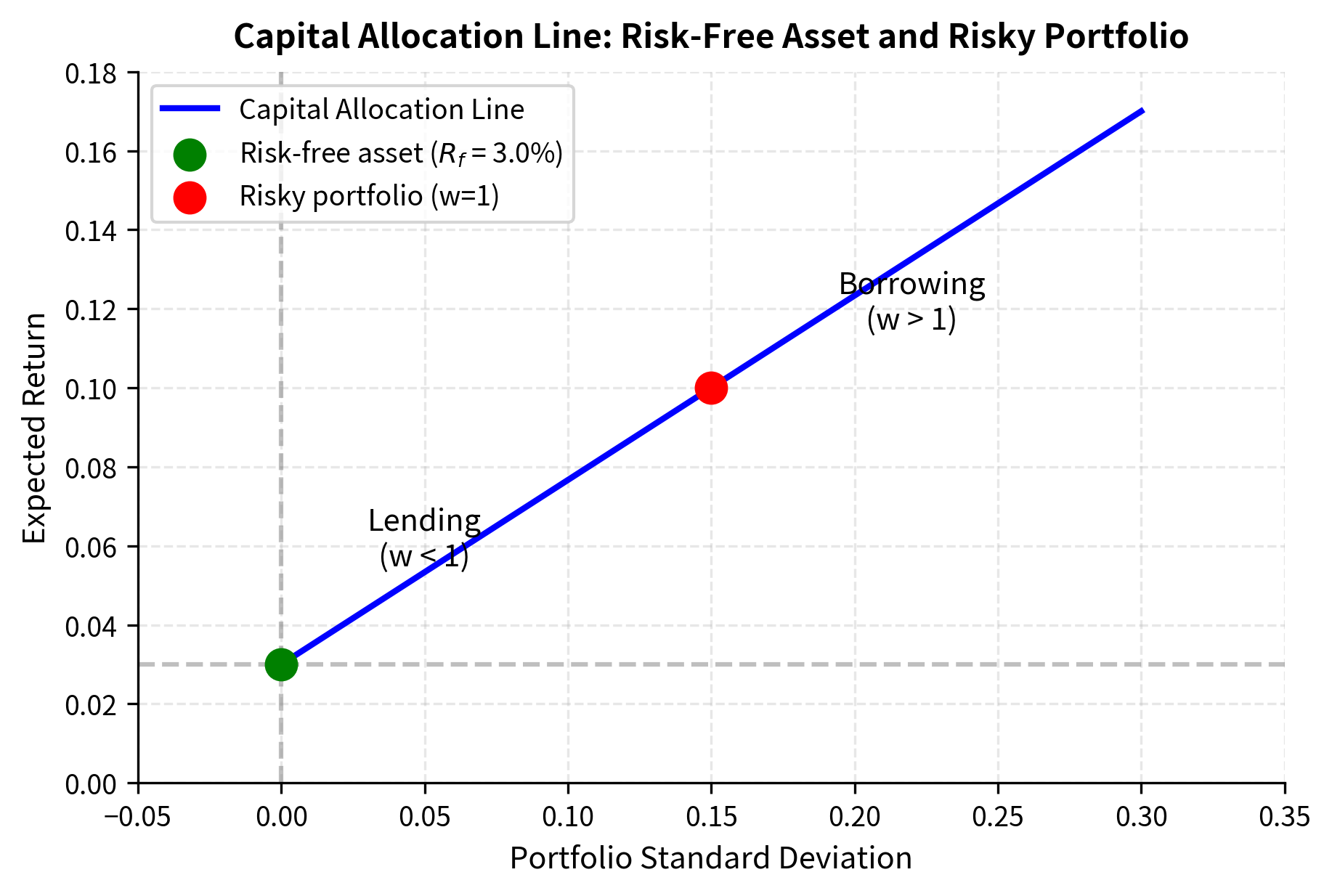
The figure illustrates how the Capital Allocation Line (CAL) extends from the risk-free rate through the risky portfolio and beyond. Investors with low risk tolerance choose portfolios close to the risk-free asset (lending portfolios), while aggressive investors leverage their positions by borrowing at the risk-free rate. The key insight is that the CAL represents all achievable combinations using a particular risky portfolio. Your optimal point on this line depends on your personal risk preferences, but everyone faces the same menu of options defined by this straight line.

The Capital Market Line and Market PortfolioLink Copied

Given that combinations with the risk-free asset create straight lines, which risky portfolio should you choose? The answer is the portfolio that creates the steepest possible line, since this provides the highest expected return per unit of risk. This observation leads us to one of CAPM's most important conclusions: you should hold the same risky portfolio.

Capital Market Line

The Capital Market Line (CML) is the straight line extending from the risk-free rate through the tangency portfolio on the efficient frontier. It represents the highest achievable Sharpe ratio and dominates all other capital allocation lines.

To understand why the tangency portfolio is optimal, imagine drawing multiple straight lines from the risk-free rate, each passing through a different risky portfolio on the efficient frontier. Each line represents a Capital Allocation Line for that particular risky portfolio. The line with the steepest slope offers the best risk-return tradeoff because you get more expected return for each unit of risk you bear. Geometrically, the steepest line is the one that is tangent to the efficient frontier, touching it at exactly one point without crossing it.

Graphically, the optimal risky portfolio is found by drawing a line from the risk-free rate tangent to the efficient frontier of risky assets. This tangency portfolio, combined with the risk-free asset, dominates all other portfolio combinations. Any other risky portfolio would create a capital allocation line with a lower slope, meaning inferior risk-adjusted returns. Choosing any other risky portfolio would leave money on the table, accepting less expected return for the same amount of risk.

In equilibrium under CAPM assumptions, all investors hold the same tangency portfolio because they all have homogeneous expectations and face the same risk-free rate. Since markets must clear (all assets must be held by someone), this tangency portfolio must be the market portfolio, the value-weighted portfolio of all risky assets in the economy. This is the aggregation insight of CAPM: when we combine our portfolios, we must get the total market. If all investors hold the same risky portfolio, that portfolio must contain all risky assets in proportion to their market values.

Market Portfolio

The market portfolio contains all risky assets in the economy, with each asset weighted by its market capitalization relative to total market capitalization. In theory, this includes stocks, bonds, real estate, human capital, and all other investable assets. In practice, broad market indices like the S&P 500 or MSCI World serve as proxies.

The Capital Market Line equation describes the risk-return relationship for efficient portfolios, which are portfolios that lie on the CML:

E[R_P] = R_f + \frac{E[R_M] - R_f}{\sigma_M} \sigma_P

where:

$E[R_P]$ : expected return of an efficient portfolio
$R_f$ : risk-free rate
$E[R_M]$ : expected return of the market portfolio
$\sigma_M$ : standard deviation of the market portfolio
$\sigma_P$ : standard deviation of the efficient portfolio

This equation tells us that for portfolios along the CML, expected return increases linearly with total risk (standard deviation). The rate of exchange between risk and return is determined by the market's risk-return characteristics.

The slope of the CML is:

\text{Sharpe\_Ratio} = \frac{E[R_M] - R_f}{\sigma_M}

where:

$E[R_M]$ : expected return of the market
$R_f$ : risk-free rate
$\sigma_M$ : market volatility

This is the market's reward-to-variability ratio, or Sharpe ratio. It represents the equilibrium price of risk in the market and indicates how much additional expected return you receive for taking on one additional unit of total risk. Named after William Sharpe, one of CAPM's developers, this ratio has become the standard measure for evaluating risk-adjusted performance. When the Sharpe ratio is 0.5, for example, investors earn 0.5% additional expected return for each 1% of additional volatility they accept.

In[4]:

Code

import numpy as np
from scipy.optimize import minimize

# Generate random assets and efficient frontier
np.random.seed(42)
n_assets = 30
expected_returns = np.random.uniform(0.04, 0.14, n_assets)
volatilities = np.random.uniform(0.10, 0.35, n_assets)

# Generate correlation matrix and covariance matrix
correlations = np.random.uniform(0.2, 0.6, (n_assets, n_assets))
correlations = (correlations + correlations.T) / 2
np.fill_diagonal(correlations, 1.0)
cov_matrix = np.outer(volatilities, volatilities) * correlations


# Find efficient frontier through optimization
def portfolio_return(weights, returns):
    return np.dot(weights, returns)


def portfolio_volatility(weights, cov_matrix):
    return np.sqrt(weights @ cov_matrix @ weights)


def neg_sharpe_ratio(weights, returns, cov_matrix, rf):
    ret = portfolio_return(weights, returns)
    vol = portfolio_volatility(weights, cov_matrix)
    return -(ret - rf) / vol


# Find tangency portfolio (maximum Sharpe ratio)
rf = 0.03
constraints = {"type": "eq", "fun": lambda w: np.sum(w) - 1}
bounds = tuple((0, 1) for _ in range(n_assets))
initial_weights = np.ones(n_assets) / n_assets

result = minimize(
    neg_sharpe_ratio,
    initial_weights,
    args=(expected_returns, cov_matrix, rf),
    method="SLSQP",
    bounds=bounds,
    constraints=constraints,
)
tangency_weights = result.x
tangency_return = portfolio_return(tangency_weights, expected_returns)
tangency_vol = portfolio_volatility(tangency_weights, cov_matrix)

# Generate efficient frontier
target_returns = np.linspace(0.04, 0.13, 50)
frontier_vols = []

for target in target_returns:
    constraints = [
        {"type": "eq", "fun": lambda w: np.sum(w) - 1},
        {
            "type": "eq",
            "fun": lambda w, t=target: portfolio_return(w, expected_returns)
            - t,
        },
    ]
    result = minimize(
        portfolio_volatility,
        initial_weights,
        args=(cov_matrix,),
        method="SLSQP",
        bounds=bounds,
        constraints=constraints,
    )
    frontier_vols.append(result.fun)

frontier_vols = np.array(frontier_vols)

import numpy as np
from scipy.optimize import minimize

# Generate random assets and efficient frontier
np.random.seed(42)
n_assets = 30
expected_returns = np.random.uniform(0.04, 0.14, n_assets)
volatilities = np.random.uniform(0.10, 0.35, n_assets)

# Generate correlation matrix and covariance matrix
correlations = np.random.uniform(0.2, 0.6, (n_assets, n_assets))
correlations = (correlations + correlations.T) / 2
np.fill_diagonal(correlations, 1.0)
cov_matrix = np.outer(volatilities, volatilities) * correlations


# Find efficient frontier through optimization
def portfolio_return(weights, returns):
    return np.dot(weights, returns)


def portfolio_volatility(weights, cov_matrix):
    return np.sqrt(weights @ cov_matrix @ weights)


def neg_sharpe_ratio(weights, returns, cov_matrix, rf):
    ret = portfolio_return(weights, returns)
    vol = portfolio_volatility(weights, cov_matrix)
    return -(ret - rf) / vol


# Find tangency portfolio (maximum Sharpe ratio)
rf = 0.03
constraints = {"type": "eq", "fun": lambda w: np.sum(w) - 1}
bounds = tuple((0, 1) for _ in range(n_assets))
initial_weights = np.ones(n_assets) / n_assets

result = minimize(
    neg_sharpe_ratio,
    initial_weights,
    args=(expected_returns, cov_matrix, rf),
    method="SLSQP",
    bounds=bounds,
    constraints=constraints,
)
tangency_weights = result.x
tangency_return = portfolio_return(tangency_weights, expected_returns)
tangency_vol = portfolio_volatility(tangency_weights, cov_matrix)

# Generate efficient frontier
target_returns = np.linspace(0.04, 0.13, 50)
frontier_vols = []

for target in target_returns:
    constraints = [
        {"type": "eq", "fun": lambda w: np.sum(w) - 1},
        {
            "type": "eq",
            "fun": lambda w, t=target: portfolio_return(w, expected_returns)
            - t,
        },
    ]
    result = minimize(
        portfolio_volatility,
        initial_weights,
        args=(cov_matrix,),
        method="SLSQP",
        bounds=bounds,
        constraints=constraints,
    )
    frontier_vols.append(result.fun)

frontier_vols = np.array(frontier_vols)

The following plot displays the efficient frontier and the Capital Market Line, highlighting the tangency portfolio.

Out[5]:

Visualization

Chart showing efficient frontier curve with tangent Capital Market Line from risk-free rate through market portfolio. — The Capital Market Line (CML) and efficient frontier. The CML (red line) originates at the risk-free rate and falls tangent to the efficient frontier at the Market Portfolio, representing the optimal risk-return tradeoff. Rational investors choose portfolios along this line by combining the risk-free asset with the market portfolio.

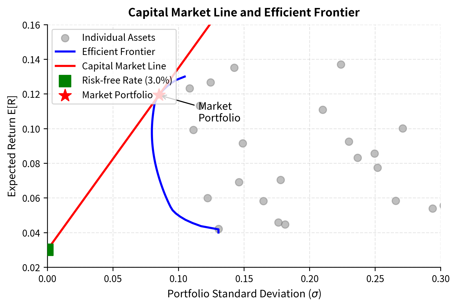
The figure shows how the CML dominates the efficient frontier of risky assets alone. Any point on the CML (except the tangency point itself) offers either higher return for the same risk or lower risk for the same return compared to the efficient frontier. This dominance is the geometric representation of the benefit from adding a risk-free asset to the investment opportunity set. The CML essentially "lifts" investors above the constraints imposed by the curved efficient frontier, offering superior combinations at every risk level except at the tangency point itself.

Systematic and Unsystematic RiskLink Copied

A crucial insight of CAPM is the decomposition of total risk into two components: systematic risk and unsystematic risk. This decomposition explains why diversification reduces portfolio risk and why the market only rewards one type of risk. Understanding this distinction is essential because it determines which risks you should care about and which risks you can safely ignore.

Systematic Risk

Systematic risk (also called market risk or non-diversifiable risk) affects all assets in the economy. It arises from macroeconomic factors like interest rate changes, recessions, inflation, and geopolitical events. Because all assets are exposed to these factors, systematic risk cannot be eliminated through diversification.

Unsystematic Risk

Unsystematic risk (also called idiosyncratic risk, specific risk, or diversifiable risk) affects only individual assets or small groups of assets. Examples include management decisions, product failures, lawsuits, and labor disputes. Unsystematic risk can be eliminated through diversification.

The intuition behind this decomposition is straightforward. When a recession hits, nearly all companies suffer to some degree, so holding more stocks doesn't protect you from recessions. That is systematic risk. But when a single company's CEO resigns unexpectedly, other companies are largely unaffected. If you hold many stocks, the bad surprises at some companies tend to be offset by good surprises at others. That is unsystematic risk, and it averages out in a diversified portfolio.

Consider a simple model where each asset's return depends on a market factor plus an asset-specific component. This single-factor structure captures the idea that all assets respond to common market conditions while also having their own unique sources of variation:

R_i = \alpha_i + \beta_i R_M + \epsilon_i

where:

$R_i$ : return on asset $i$
$\alpha_i$ : asset's return component independent of the market
$\beta_i$ : sensitivity to market movements
$R_M$ : market return
$\epsilon_i$ : idiosyncratic component (with $E[\epsilon_i] = 0$ and $Cov(\epsilon_i, R_M) = 0$ )

This model states that an asset's return can be decomposed into three parts: a constant component $\alpha_i$ that represents the asset's baseline expected return unrelated to the market, a systematic component $\beta_i R_M$ that moves with the market, and an idiosyncratic component $\epsilon_i$ that captures firm-specific events. The key assumption is that the idiosyncratic component is uncorrelated with market returns, meaning firm-specific shocks are independent of broader economic conditions.

Using the properties of variance and the assumption that $Cov(\epsilon_i, R_M) = 0$ , we decompose the total variance. This derivation applies the standard variance formula for a sum of random variables, recognizing that the constant term $\alpha_i$ contributes nothing to variance and that the cross-term vanishes due to the independence assumption:

\begin{aligned} \sigma_i^2 &= Var(R_i) \\ &= Var(\alpha_i + \beta_i R_M + \epsilon_i) && \text{(substitute return model)} \\ &= \beta_i^2 Var(R_M) + Var(\epsilon_i) + 2\beta_i Cov(R_M, \epsilon_i) && \text{(variance properties)} \\ &= \beta_i^2 \sigma_M^2 + \sigma_{\epsilon_i}^2 && \text{(uncorrelated residuals)} \end{aligned}

where:

$\sigma_i^2$ : total variance of asset $i$
$\beta_i^2 \sigma_M^2$ : systematic variance (market risk)
$\sigma_{\epsilon_i}^2$ : unsystematic variance (idiosyncratic risk)

The first term represents systematic variance (exposure to market risk), while the second term represents unsystematic variance. The decomposition shows that total variance splits cleanly into two additive components. The systematic component depends on the square of beta (measuring how strongly the asset responds to market movements) times the market variance. The unsystematic component is simply the variance of the firm-specific shocks.

We can visualize this decomposition for a set of hypothetical assets to see how the proportions of systematic and unsystematic risk vary across different types of securities.

Out[7]:

Visualization

Stacked bar chart showing systematic and unsystematic variance for different asset types. — Decomposition of total variance into systematic and unsystematic components for different asset types. The market index has only systematic risk, while individual stocks carry substantial idiosyncratic risk. Diversified portfolios reduce the unsystematic component.

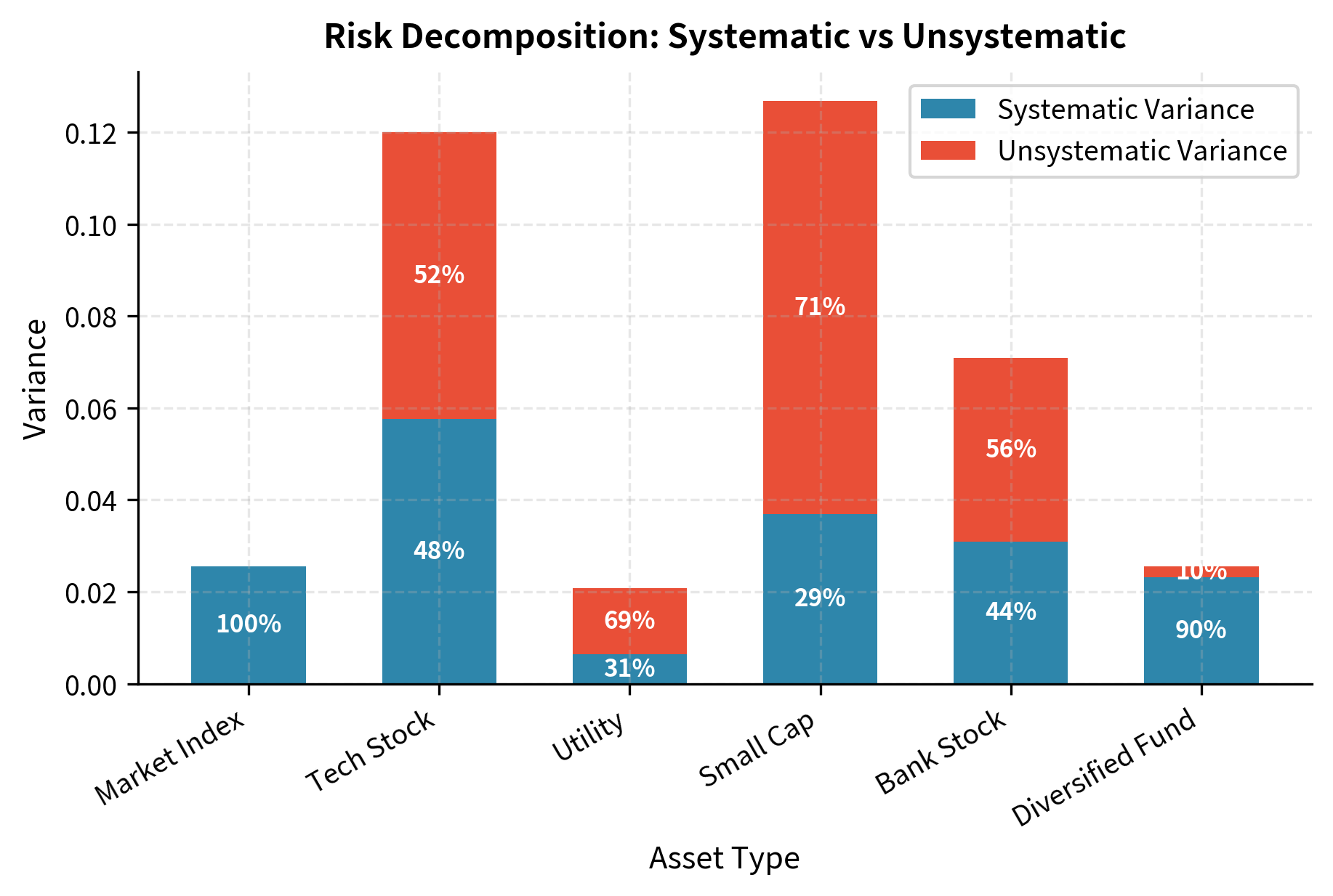
In a well-diversified portfolio, the unsystematic risks of individual assets cancel out through diversification, leaving only systematic risk. To see why, consider an equally-weighted portfolio of $n$ stocks. The portfolio's idiosyncratic variance equals the average of the individual idiosyncratic variances divided by $n$ . As $n$ grows large, this term approaches zero. However, the systematic component does not diversify away because all stocks share exposure to the same market factor.

In[8]:

Code

import numpy as np

# Demonstrate diversification effect
np.random.seed(123)

# Simulate returns for many assets
n_assets_sim = 500
n_periods = 252  # One year of daily returns

# Market returns
market_returns = np.random.normal(
    0.0004, 0.01, n_periods
)  # ~10% annual, 16% vol

# Asset-specific parameters
betas = np.random.uniform(0.5, 1.5, n_assets_sim)
idio_vols = np.random.uniform(
    0.005, 0.02, n_assets_sim
)  # Daily idiosyncratic vol

# Generate asset returns
asset_returns = np.zeros((n_periods, n_assets_sim))
for i in range(n_assets_sim):
    idio_returns = np.random.normal(0, idio_vols[i], n_periods)
    asset_returns[:, i] = betas[i] * market_returns + idio_returns

# Calculate portfolio volatility for different portfolio sizes
portfolio_sizes = list(range(1, 101))
avg_volatilities = []

for n in portfolio_sizes:
    # Average over many random portfolios of size n
    vols = []
    for _ in range(100):
        selected = np.random.choice(n_assets_sim, n, replace=False)
        port_returns = asset_returns[:, selected].mean(axis=1)
        vols.append(port_returns.std() * np.sqrt(252))  # Annualized
    avg_volatilities.append(np.mean(vols))

# Theoretical systematic risk of equal-weighted portfolio
market_vol = market_returns.std() * np.sqrt(252)
systematic_risk = market_vol * betas.mean()  # Average beta times market vol

import numpy as np

# Demonstrate diversification effect
np.random.seed(123)

# Simulate returns for many assets
n_assets_sim = 500
n_periods = 252  # One year of daily returns

# Market returns
market_returns = np.random.normal(
    0.0004, 0.01, n_periods
)  # ~10% annual, 16% vol

# Asset-specific parameters
betas = np.random.uniform(0.5, 1.5, n_assets_sim)
idio_vols = np.random.uniform(
    0.005, 0.02, n_assets_sim
)  # Daily idiosyncratic vol

# Generate asset returns
asset_returns = np.zeros((n_periods, n_assets_sim))
for i in range(n_assets_sim):
    idio_returns = np.random.normal(0, idio_vols[i], n_periods)
    asset_returns[:, i] = betas[i] * market_returns + idio_returns

# Calculate portfolio volatility for different portfolio sizes
portfolio_sizes = list(range(1, 101))
avg_volatilities = []

for n in portfolio_sizes:
    # Average over many random portfolios of size n
    vols = []
    for _ in range(100):
        selected = np.random.choice(n_assets_sim, n, replace=False)
        port_returns = asset_returns[:, selected].mean(axis=1)
        vols.append(port_returns.std() * np.sqrt(252))  # Annualized
    avg_volatilities.append(np.mean(vols))

# Theoretical systematic risk of equal-weighted portfolio
market_vol = market_returns.std() * np.sqrt(252)
systematic_risk = market_vol * betas.mean()  # Average beta times market vol

We plot the average portfolio volatility against the number of holdings to visualize the diversification benefit.

Out[9]:

Visualization

Line chart showing portfolio volatility decreasing and leveling off as number of holdings increases. — Portfolio volatility decreases as the number of holdings increases, but converges to the systematic risk level. Beyond approximately 30-40 stocks, additional diversification provides minimal risk reduction.

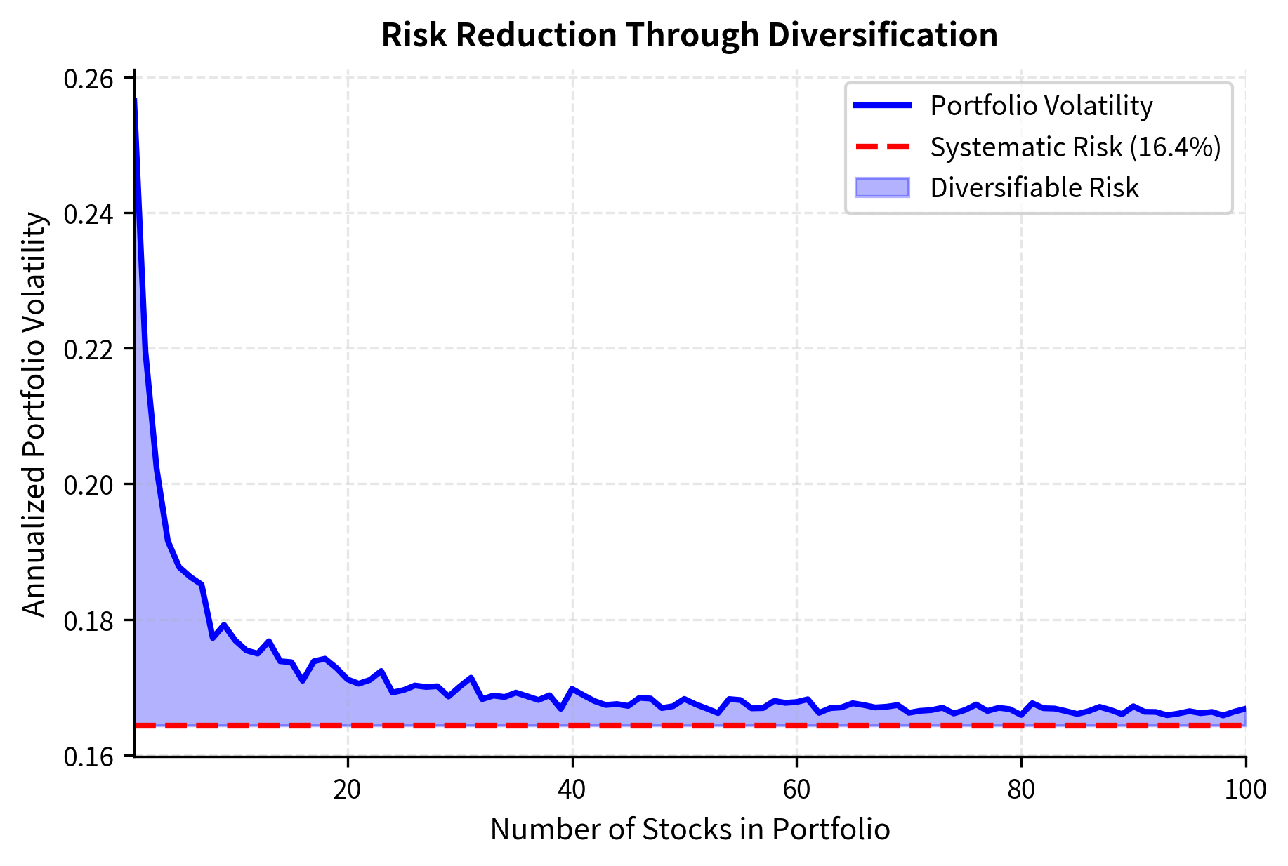
The figure demonstrates a fundamental principle: while adding more securities to a portfolio reduces total volatility, there's a floor below which risk cannot be reduced. This floor is the systematic risk component. The shaded area represents diversifiable risk, the portion of total volatility that disappears as you add more securities. Notice how quickly the curve drops initially; the first few securities you add provide substantial risk reduction. But the curve flattens out around 30 to 40 stocks, indicating diminishing returns to further diversification.

Since investors can eliminate unsystematic risk at no cost through diversification, the market provides no compensation for bearing it. Only systematic risk commands a risk premium. This insight is the economic foundation of CAPM. If you could earn extra return by bearing idiosyncratic risk, every investor would pile into high-idiosyncratic-risk stocks until prices rose and expected returns fell to the level justified by systematic risk alone.

Beta: The Measure of Systematic RiskLink Copied

Beta ( $\beta$ ) quantifies an asset's systematic risk by measuring its sensitivity to market movements. It is the central risk measure in CAPM and the key input for determining an asset's required return. While standard deviation measures total risk, beta isolates the portion of risk that matters for pricing.

Beta

Beta measures the expected change in an asset's return for a 1% change in the market return. Mathematically, it equals the covariance of the asset's return with the market return, divided by the variance of the market return:

\beta_i = \frac{Cov(R_i, R_M)}{Var(R_M)} = \frac{\sigma_{i,M}}{\sigma_M^2}

where:

$\beta_i$ : beta of asset $i$
$Cov(R_i, R_M)$ or $\sigma_{i,M}$ : covariance between asset and market returns
$Var(R_M)$ or $\sigma_M^2$ : variance of market returns

The formula for beta can be understood through regression analysis. If you regress an asset's returns on market returns, the slope coefficient is exactly beta. The covariance in the numerator measures how strongly the asset moves with the market, while the variance in the denominator normalizes by the market's own variability. This normalization ensures that beta measures relative sensitivity rather than absolute comovement.

The beta of the market portfolio itself is exactly 1 by definition. To verify this, note that when calculating the market's beta, the numerator becomes $Cov(R_M, R_M) = Var(R_M)$ , which exactly cancels the denominator. Assets with different betas exhibit distinct behaviors:

$\beta > 1$ (aggressive assets): More volatile than the market. Technology stocks, small caps, and high-growth companies typically have betas above 1. They amplify market movements, rising more than the market in good times but falling more in bad times. If you seek higher expected returns and are willing to accept greater market sensitivity, you would tilt toward high-beta assets.
$\beta = 1$ (neutral assets): Move in line with the market. A diversified market index has beta of exactly 1. These assets provide average market exposure without amplification or dampening.
$0 < \beta < 1$ (defensive assets): Less volatile than the market. Utilities, consumer staples, and healthcare stocks often have betas below 1. They dampen market movements, providing more stable returns that don't swing as dramatically with market conditions. If you seek stability relative to the market, you favor defensive assets.
$\beta = 0$ (zero-beta assets): Uncorrelated with the market. The risk-free asset has zero beta. Some hedge fund strategies aim for zero beta to generate returns independent of market direction. These assets provide diversification benefits but, according to CAPM, should earn only the risk-free rate.
$\beta < 0$ (negative beta): Move opposite to the market. Gold and some defensive assets occasionally exhibit negative beta. These provide natural hedges against market downturns, potentially generating positive returns when the market falls. Negative-beta assets are rare and valuable for portfolio construction.

Beta has an important portfolio property that makes it particularly useful for investment management: the beta of a portfolio equals the weighted average of its component betas:

\beta_P = \sum_{i=1}^{n} w_i \beta_i

where:

$\beta_P$ : beta of the portfolio
$n$ : number of assets in the portfolio
$w_i$ : weight of asset $i$ in the portfolio
$\beta_i$ : beta of asset $i$

This additivity property follows from the linearity of covariance. It allows portfolio managers to easily calculate and target specific beta exposures. If you want a portfolio with beta of 0.8, you can achieve this by appropriately weighting assets with different individual betas. This makes beta a practical tool for controlling systematic risk exposure.

In[10]:

Code

import numpy as np

# Illustrate different beta behaviors
np.random.seed(456)
n_periods_demo = 100

# Market returns
market_demo = np.cumsum(np.random.normal(0.001, 0.015, n_periods_demo))

# Create assets with different betas
betas_demo = [1.5, 1.0, 0.5, 0.0, -0.3]
labels = [
    "β=1.5 (Aggressive)",
    "β=1.0 (Market)",
    "β=0.5 (Defensive)",
    "β=0 (Zero-beta)",
    "β=-0.3 (Negative)",
]
colors = ["red", "black", "blue", "gray", "purple"]

market_changes = np.diff(market_demo)
asset_paths = [market_demo]  # Market is first

for b in [1.5, 0.5, 0.0, -0.3]:
    idio_noise = np.random.normal(0, 0.008, n_periods_demo - 1)
    asset_changes = b * market_changes + idio_noise
    asset_path = np.concatenate([[0], np.cumsum(asset_changes)])
    asset_paths.append(asset_path)

import numpy as np

# Illustrate different beta behaviors
np.random.seed(456)
n_periods_demo = 100

# Market returns
market_demo = np.cumsum(np.random.normal(0.001, 0.015, n_periods_demo))

# Create assets with different betas
betas_demo = [1.5, 1.0, 0.5, 0.0, -0.3]
labels = [
    "β=1.5 (Aggressive)",
    "β=1.0 (Market)",
    "β=0.5 (Defensive)",
    "β=0 (Zero-beta)",
    "β=-0.3 (Negative)",
]
colors = ["red", "black", "blue", "gray", "purple"]

market_changes = np.diff(market_demo)
asset_paths = [market_demo]  # Market is first

for b in [1.5, 0.5, 0.0, -0.3]:
    idio_noise = np.random.normal(0, 0.008, n_periods_demo - 1)
    asset_changes = b * market_changes + idio_noise
    asset_path = np.concatenate([[0], np.cumsum(asset_changes)])
    asset_paths.append(asset_path)

By plotting the cumulative returns, we can see how the different beta values affect asset performance relative to the market.

Out[11]:

Visualization

Line chart showing cumulative returns of assets with different betas responding to market movements. — Cumulative returns for assets with varying betas over a simulated period. The high-beta asset (red, β=1.5) amplifies market movements, exhibiting larger gains and losses than the market (black, β=1.0). In contrast, the negative-beta asset (purple, β=-0.3) moves inversely to the market, providing diversification benefits.

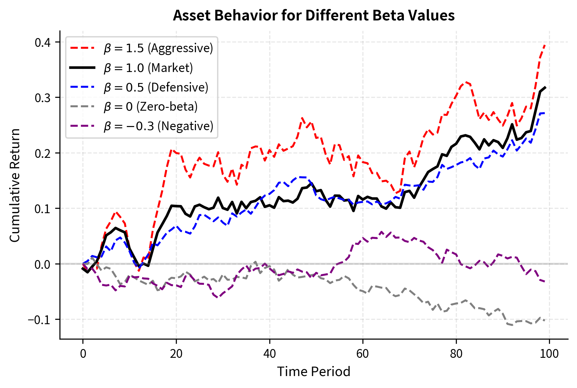
The chart shows how assets with different betas respond to the same market environment. The high-beta asset exaggerates market movements (both gains and losses), while the defensive asset moves more modestly. The negative-beta asset provides diversification by moving against the market trend. Notice that when the market rises, the aggressive asset rises even more, but when the market falls, the aggressive asset falls more steeply. The zero-beta asset wanders independently, driven entirely by its idiosyncratic component.

The Security Market LineLink Copied

While the Capital Market Line describes the risk-return relationship for efficient portfolios, the Security Market Line (SML) describes the relationship for all individual assets and portfolios, efficient or not. This is a crucial distinction. The CML tells us about portfolios that combine the risk-free asset with the market portfolio. The SML tells us about any asset, regardless of whether it is efficiently priced or part of an optimal portfolio.

Security Market Line

The Security Market Line shows the linear relationship between expected return and systematic risk (beta) for all assets in equilibrium. Its equation is the CAPM formula:

E[R_i] = R_f + \beta_i (E[R_M] - R_f)

where:

$E[R_i]$ : required/expected return on asset $i$
$R_f$ : risk-free rate of return
$\beta_i$ : systematic risk of asset $i$
$E[R_M]$ : expected return of the market portfolio
$E[R_M] - R_f$ : market risk premium

The key difference between the CML and SML lies in the risk measure used:

CML uses total risk (standard deviation $\sigma$ ) and applies only to efficient portfolios
SML uses systematic risk (beta $\beta$ ) and applies to all assets and portfolios

This difference reflects a fundamental insight. For efficient portfolios, which have no idiosyncratic risk, total risk and systematic risk are proportional. But for individual assets or inefficient portfolios, total risk includes both systematic and idiosyncratic components. Only the systematic component determines expected return, so beta is the appropriate risk measure for pricing individual securities.

The intuition behind the SML is powerful: since unsystematic risk can be diversified away at no cost, investors should not expect compensation for bearing it. The market only compensates investors for systematic risk exposure. An asset's expected return depends solely on its beta, not on its total volatility. Two assets with identical betas should have identical expected returns, even if one has much higher total volatility due to idiosyncratic risk.

The term $E[R_M] - R_f$ is called the market risk premium or equity risk premium. It represents the extra return investors demand for holding the risky market portfolio instead of the risk-free asset. Historical estimates for the U.S. market range from 4% to 8% annually, though this is subject to considerable debate. The market risk premium reflects our aggregate risk aversion, as a more risk-averse investor population would demand a higher premium for bearing market risk.

The SML equation provides a benchmark for evaluating any investment. If an asset's expected return exceeds the SML prediction given its beta, it offers more return than required for its risk level, making it attractive. If an asset's expected return falls below the SML prediction, it fails to compensate adequately for its systematic risk and should be avoided or sold.

In[12]:

Code

import numpy as np

# Create SML plot with assets
rf_sml = 0.03
market_premium = 0.06  # 6% market risk premium
market_return_sml = rf_sml + market_premium

# Generate hypothetical assets
np.random.seed(789)
n_assets_sml = 25
asset_betas = np.random.uniform(0, 2, n_assets_sml)
# True expected returns from CAPM
capm_expected = rf_sml + asset_betas * market_premium
# Actual returns with some noise (representing estimation error or mispricing)
actual_returns = capm_expected + np.random.normal(0, 0.015, n_assets_sml)

# SML line
sml_betas = np.linspace(0, 2.2, 100)
sml_returns = rf_sml + sml_betas * market_premium

import numpy as np

# Create SML plot with assets
rf_sml = 0.03
market_premium = 0.06  # 6% market risk premium
market_return_sml = rf_sml + market_premium

# Generate hypothetical assets
np.random.seed(789)
n_assets_sml = 25
asset_betas = np.random.uniform(0, 2, n_assets_sml)
# True expected returns from CAPM
capm_expected = rf_sml + asset_betas * market_premium
# Actual returns with some noise (representing estimation error or mispricing)
actual_returns = capm_expected + np.random.normal(0, 0.015, n_assets_sml)

# SML line
sml_betas = np.linspace(0, 2.2, 100)
sml_returns = rf_sml + sml_betas * market_premium

The Security Market Line visualizes this relationship, helping us identify undervalued and overvalued assets.

Out[13]:

Visualization

Scatter plot of assets with different betas and returns, with Security Market Line showing equilibrium relationship. — The Security Market Line (SML) displays the equilibrium relationship between systematic risk (beta) and expected return. Assets plotting above the blue SML indicate positive alpha (undervaluation), offering higher returns than required for their risk level. Conversely, assets below the line indicate negative alpha (overvaluation).

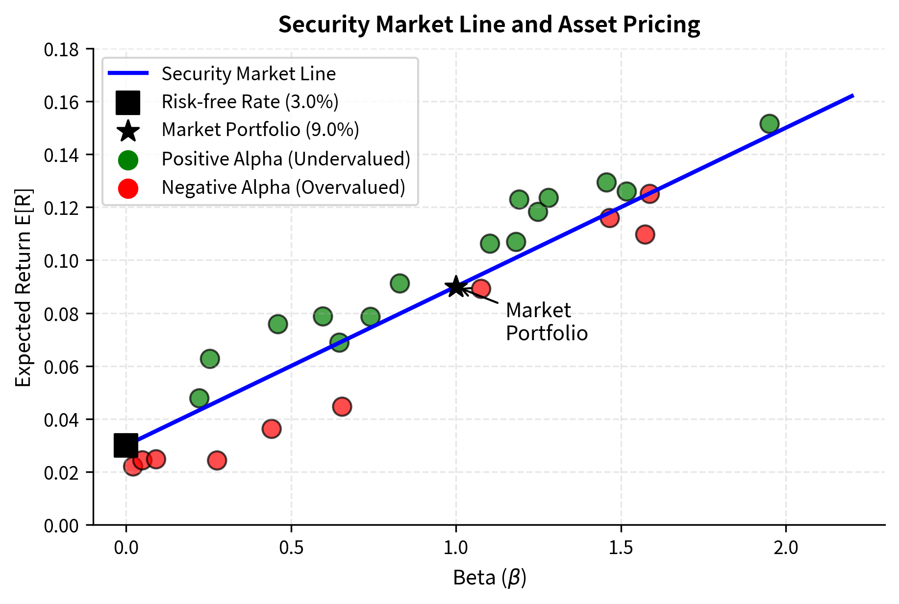
The chart visually distinguishes between properly priced, undervalued, and overvalued assets. Assets lying on the SML are in equilibrium, while those above the line (green) offer returns superior to CAPM predictions (positive alpha), and those below (red) fail to compensate adequately for their systematic risk. The vertical distance from each asset to the line represents the magnitude of its mispricing. You would seek to buy assets above the line and sell or avoid assets below it.

Alpha: Measuring Abnormal ReturnsLink Copied

Alpha represents the return on an asset or portfolio beyond what CAPM predicts given its systematic risk exposure. It measures performance after adjusting for beta risk. While beta tells us about risk exposure, alpha tells us about value creation or destruction relative to that risk exposure.

Alpha

Alpha ( $\alpha$ ) is the difference between an asset's actual return and its CAPM-predicted return:

\alpha_i = R_i - [R_f + \beta_i(R_M - R_f)]

where:

$\alpha_i$ : alpha (abnormal return) of asset $i$
$R_i$ : realized return of asset $i$
$R_f$ : risk-free rate
$\beta_i$ : beta of asset $i$
$R_M$ : realized market return
$R_f + \beta_i(R_M - R_f)$ : CAPM-predicted return given realized market return

Positive alpha indicates outperformance relative to the asset's risk level; negative alpha indicates underperformance.

The formula for alpha captures a simple but profound idea. We first calculate what return the asset should have earned given the market conditions and its systematic risk exposure. Then we compare this benchmark return to what the asset actually earned. The difference, alpha, represents the value added or subtracted beyond what beta exposure alone would explain.

In an efficient market where CAPM holds perfectly, all assets should have zero alpha; assets should be priced fairly given their systematic risk. Alpha represents either:

Market mispricing: Temporary deviations from fair value that you can exploit. If an asset is underpriced, its realized return will exceed the CAPM prediction, generating positive alpha. As prices correct, the alpha opportunity disappears.
Risk not captured by beta: Exposure to factors not included in CAPM's single-factor model. An asset might earn high returns because it loads on additional risk factors (like size or value) that CAPM ignores. This alpha is not necessarily due to mispricing but rather to model misspecification.
Luck or statistical noise: Random variation that appears as skill. Any finite sample will show some assets with positive and negative alpha purely by chance, even if all assets are fairly priced in expectation.

Alpha is central to investment management. Active managers aim to generate positive alpha by identifying mispriced securities or timing market movements. The challenge is distinguishing genuine skill from luck, a topic we'll explore in detail in the chapter on Portfolio Performance Measurement. A manager who consistently generates positive alpha demonstrates investment skill, but alpha estimates are noisy and require long track records to evaluate reliably.

For portfolios, alpha can be generated through:

Security selection: Choosing undervalued securities (positive-alpha assets). This involves fundamental analysis to identify stocks trading below intrinsic value.
Market timing: Adjusting beta exposure based on market forecasts. Increasing beta before market rallies and decreasing it before declines generates alpha if timing is accurate.
Factor tilts: Exposure to rewarded factors beyond the market factor. Tilting toward small-cap, value, or momentum stocks may generate apparent alpha if these factors are not explicitly accounted for in the benchmark.

In[14]:

Code

import pandas as pd

# Calculate alpha for a sample of stocks
# Using simulated data as if we ran regressions

stock_names = [
    "AAPL",
    "MSFT",
    "AMZN",
    "GOOGL",
    "META",
    "NVDA",
    "TSLA",
    "JPM",
    "JNJ",
    "PG",
]
stock_betas = [1.25, 1.15, 1.30, 1.10, 1.35, 1.50, 1.80, 1.20, 0.65, 0.55]
# Actual returns over the period
actual_stock_returns = [
    0.15,
    0.12,
    0.18,
    0.11,
    0.08,
    0.25,
    0.20,
    0.10,
    0.09,
    0.08,
]

rf_period = 0.04  # 4% risk-free over period
market_return_period = 0.10  # 10% market return over period
market_premium_period = market_return_period - rf_period

# Calculate expected returns and alphas
expected_stock_returns = [
    rf_period + b * market_premium_period for b in stock_betas
]
stock_alphas = [
    actual - expected
    for actual, expected in zip(actual_stock_returns, expected_stock_returns)
]

alpha_df = pd.DataFrame(
    {
        "Stock": stock_names,
        "Beta": stock_betas,
        "Actual Return": [f"{r:.2%}" for r in actual_stock_returns],
        "CAPM Expected": [f"{r:.2%}" for r in expected_stock_returns],
        "Alpha": [f"{a:+.2%}" for a in stock_alphas],
    }
)

import pandas as pd

# Calculate alpha for a sample of stocks
# Using simulated data as if we ran regressions

stock_names = [
    "AAPL",
    "MSFT",
    "AMZN",
    "GOOGL",
    "META",
    "NVDA",
    "TSLA",
    "JPM",
    "JNJ",
    "PG",
]
stock_betas = [1.25, 1.15, 1.30, 1.10, 1.35, 1.50, 1.80, 1.20, 0.65, 0.55]
# Actual returns over the period
actual_stock_returns = [
    0.15,
    0.12,
    0.18,
    0.11,
    0.08,
    0.25,
    0.20,
    0.10,
    0.09,
    0.08,
]

rf_period = 0.04  # 4% risk-free over period
market_return_period = 0.10  # 10% market return over period
market_premium_period = market_return_period - rf_period

# Calculate expected returns and alphas
expected_stock_returns = [
    rf_period + b * market_premium_period for b in stock_betas
]
stock_alphas = [
    actual - expected
    for actual, expected in zip(actual_stock_returns, expected_stock_returns)
]

alpha_df = pd.DataFrame(
    {
        "Stock": stock_names,
        "Beta": stock_betas,
        "Actual Return": [f"{r:.2%}" for r in actual_stock_returns],
        "CAPM Expected": [f"{r:.2%}" for r in expected_stock_returns],
        "Alpha": [f"{a:+.2%}" for a in stock_alphas],
    }
)

Out[15]:

Console

Alpha Analysis: Actual vs CAPM Expected Returns
=================================================================
Stock  Beta Actual Return CAPM Expected   Alpha
 AAPL  1.25        15.00%        11.50%  +3.50%
 MSFT  1.15        12.00%        10.90%  +1.10%
 AMZN  1.30        18.00%        11.80%  +6.20%
GOOGL  1.10        11.00%        10.60%  +0.40%
 META  1.35         8.00%        12.10%  -4.10%
 NVDA  1.50        25.00%        13.00% +12.00%
 TSLA  1.80        20.00%        14.80%  +5.20%
  JPM  1.20        10.00%        11.20%  -1.20%
  JNJ  0.65         9.00%         7.90%  +1.10%
   PG  0.55         8.00%         7.30%  +0.70%

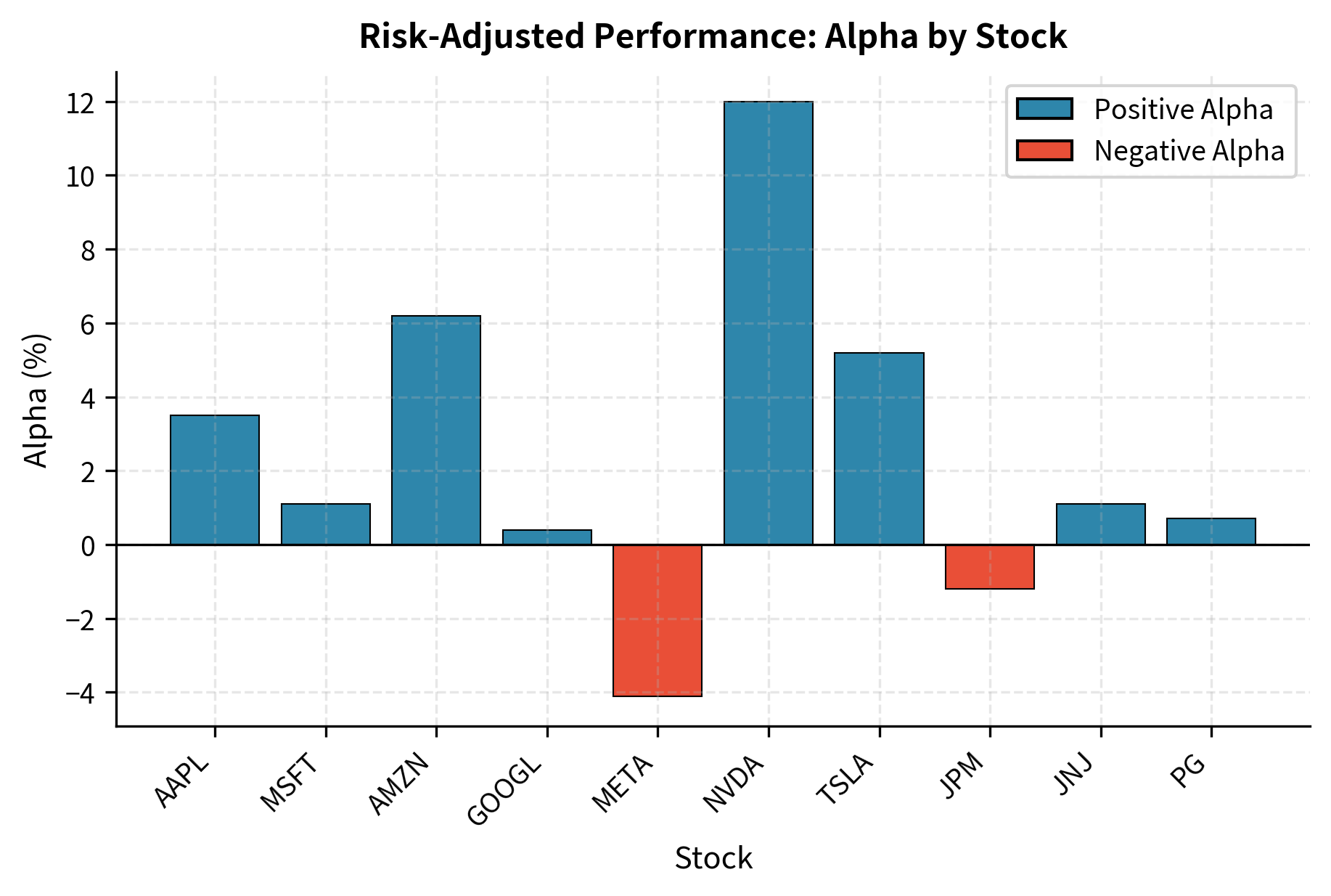
The table shows how alpha captures performance beyond what beta explains. NVDA and TSLA generated substantial positive alpha, delivering returns well above what their high betas would predict. Conversely, META underperformed its CAPM expectation, generating negative alpha despite strong beta exposure to the rising market. These results illustrate that high beta does not guarantee high returns; what matters for evaluating performance is whether returns exceed the risk-adjusted expectation.

We can visualize the distribution of alphas to see the range of risk-adjusted performance across the sample stocks.

Out[16]:

Visualization

Bar chart showing alpha values for individual stocks, with bars colored by sign. — Distribution of alpha values across sample stocks. The spread around zero indicates the variation in risk-adjusted performance, with positive alphas representing outperformance and negative alphas representing underperformance relative to CAPM predictions.

Estimating Beta in PracticeLink Copied

While beta is defined theoretically as a population parameter, you must estimate it from historical data. The standard approach uses regression analysis, as covered in our chapter on Regression Analysis for Financial Relationships. Understanding the practical aspects of beta estimation is essential because the choices made in estimation significantly affect the resulting beta values and their usefulness for forward-looking decisions.

The market model regresses an asset's excess returns on market excess returns:

R_{i,t} - R_f = \alpha_i + \beta_i(R_{M,t} - R_f) + \epsilon_{i,t}

where:

$R_{i,t} - R_f$ : excess return of asset $i$ at time $t$
$\alpha_i$ : intercept (estimated alpha)
$\beta_i$ : slope coefficient (estimated beta)
$R_{M,t} - R_f$ : excess return of the market at time $t$
$\epsilon_{i,t}$ : residual error term at time $t$

This regression directly implements the CAPM relationship. The slope coefficient $\beta_i$ estimates the asset's systematic risk, capturing how the asset's excess return responds to changes in the market's excess return. The intercept $\alpha_i$ estimates the asset's alpha, though interpreting this requires caution since estimation error can make alpha appear nonzero even when the true alpha is zero.

The slope coefficient $\beta_i$ estimates the asset's systematic risk. Several practical considerations affect beta estimation:

Estimation period: Longer periods provide more data but may include structural changes in the company. Common choices range from 2 to 5 years of monthly data or 1 to 2 years of weekly data. A company that undergoes a major acquisition or changes its business model may have a fundamentally different beta after the event than before, making historical estimates misleading.
Return frequency: Daily returns provide more observations but can be noisy due to bid-ask bounce and non-synchronous trading. Monthly returns are smoother but offer fewer observations. The choice involves a tradeoff between statistical precision (favoring more observations) and data quality (favoring less noisy observations).
Market proxy: The true market portfolio is unobservable, so practitioners use broad indices like the S&P 500, Russell 3000, or MSCI World. The choice affects beta estimates because different indices have different compositions and return characteristics. An international company's beta relative to the S&P 500 may differ from its beta relative to a global index.
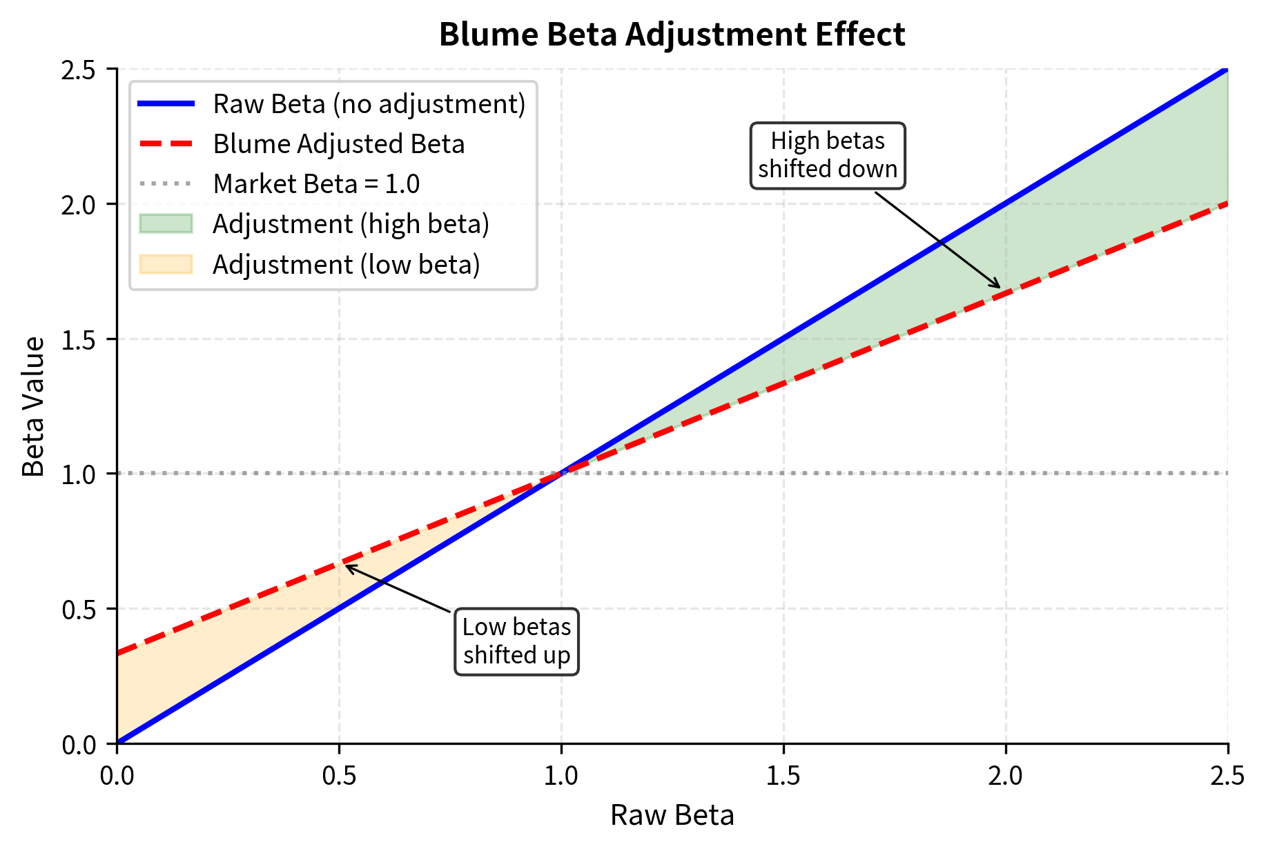
Adjusted beta: Raw betas tend to be noisy and exhibit mean reversion toward 1.0. Companies with extreme betas tend to become more average over time as they mature or as market conditions change. Bloomberg and other providers often report adjusted betas using the Blume adjustment:

\beta_{\text{adjusted}} = \frac{2}{3}\beta_{\text{raw}} + \frac{1}{3}(1.0)

where:

$\beta_{\text{adjusted}}$ : forecasted beta for the next period
$\beta_{\text{raw}}$ : historical regression beta
$1.0$ : beta of the market (mean reversion target)

This adjustment shrinks extreme betas toward the market average, reflecting the empirical observation that betas tend to converge toward 1.0 over time. The specific weights of two-thirds and one-third were determined empirically by Marshall Blume and represent an average rate of mean reversion across stocks.

We can visualize the effect of the Blume adjustment on a range of raw beta values to understand how it dampens extreme estimates.

Out[17]:

Visualization

Line chart comparing raw betas to Blume-adjusted betas across a range of values. — The Blume adjustment shrinks raw beta estimates toward 1.0, reflecting the empirical tendency of betas to mean-revert over time. Extreme betas are adjusted more aggressively than moderate betas.

In[18]:

Code

import numpy as np
from scipy import stats

# Estimate beta using simulated data (mimicking real regression)
np.random.seed(101)

# Simulate 3 years of monthly returns
n_months = 36
market_monthly = np.random.normal(
    0.008, 0.045, n_months
)  # ~10% annual return, ~15% vol
rf_monthly = 0.003  # ~3.6% annual

# Simulate a stock with true beta of 1.3
true_beta = 1.3
true_alpha = 0.0  # 0% alpha (consistent with CAPM)
idio_vol = 0.03
# Generate returns using Jensen's Alpha model: Ri = Rf + alpha + beta*(Rm - Rf) + epsilon
stock_monthly = (
    rf_monthly
    + true_alpha
    + true_beta * (market_monthly - rf_monthly)
    + np.random.normal(0, idio_vol, n_months)
)

# Excess returns
market_excess = market_monthly - rf_monthly
stock_excess = stock_monthly - rf_monthly

# OLS regression
slope, intercept, r_value, p_value, std_err = stats.linregress(
    market_excess, stock_excess
)

estimated_beta = slope
estimated_alpha = intercept
r_squared = r_value**2

# Confidence interval for beta
t_critical = stats.t.ppf(0.975, n_months - 2)  # 95% confidence
beta_ci_lower = estimated_beta - t_critical * std_err
beta_ci_upper = estimated_beta + t_critical * std_err

import numpy as np
from scipy import stats

# Estimate beta using simulated data (mimicking real regression)
np.random.seed(101)

# Simulate 3 years of monthly returns
n_months = 36
market_monthly = np.random.normal(
    0.008, 0.045, n_months
)  # ~10% annual return, ~15% vol
rf_monthly = 0.003  # ~3.6% annual

# Simulate a stock with true beta of 1.3
true_beta = 1.3
true_alpha = 0.0  # 0% alpha (consistent with CAPM)
idio_vol = 0.03
# Generate returns using Jensen's Alpha model: Ri = Rf + alpha + beta*(Rm - Rf) + epsilon
stock_monthly = (
    rf_monthly
    + true_alpha
    + true_beta * (market_monthly - rf_monthly)
    + np.random.normal(0, idio_vol, n_months)
)

# Excess returns
market_excess = market_monthly - rf_monthly
stock_excess = stock_monthly - rf_monthly

# OLS regression
slope, intercept, r_value, p_value, std_err = stats.linregress(
    market_excess, stock_excess
)

estimated_beta = slope
estimated_alpha = intercept
r_squared = r_value**2

# Confidence interval for beta
t_critical = stats.t.ppf(0.975, n_months - 2)  # 95% confidence
beta_ci_lower = estimated_beta - t_critical * std_err
beta_ci_upper = estimated_beta + t_critical * std_err

The following output summarizes the regression results, including the estimated beta and its confidence interval.

Out[19]:

Console

Beta Estimation Results
=============================================
Estimation period: 36 months
True beta: 1.30
Estimated beta: 1.418
Standard error: 0.107
95% Confidence interval: [1.200, 1.636]
Estimated alpha (monthly): 0.0060 (7.16% annualized)
R-squared: 0.837

The regression output compares the estimated parameters to the true values from our simulation. The estimated beta provides a point estimate of systematic risk, while the confidence interval defines the range where the true parameter likely lies. Notice that even with 36 months of data, the confidence interval is fairly wide, reflecting the inherent uncertainty in beta estimation. The near-zero alpha confirms that the asset was priced according to CAPM in our simulation, though in practice alpha estimates often differ from zero due to estimation error or genuine mispricing.

Out[20]:

Visualization

Scatter plot showing stock excess returns versus market excess returns with regression line. — Beta estimation using a regression of stock excess returns on market excess returns. The positive slope of the fitted line demonstrates the asset's sensitivity to market fluctuations, while the scatter of data points reflects the impact of idiosyncratic risk on realized returns.

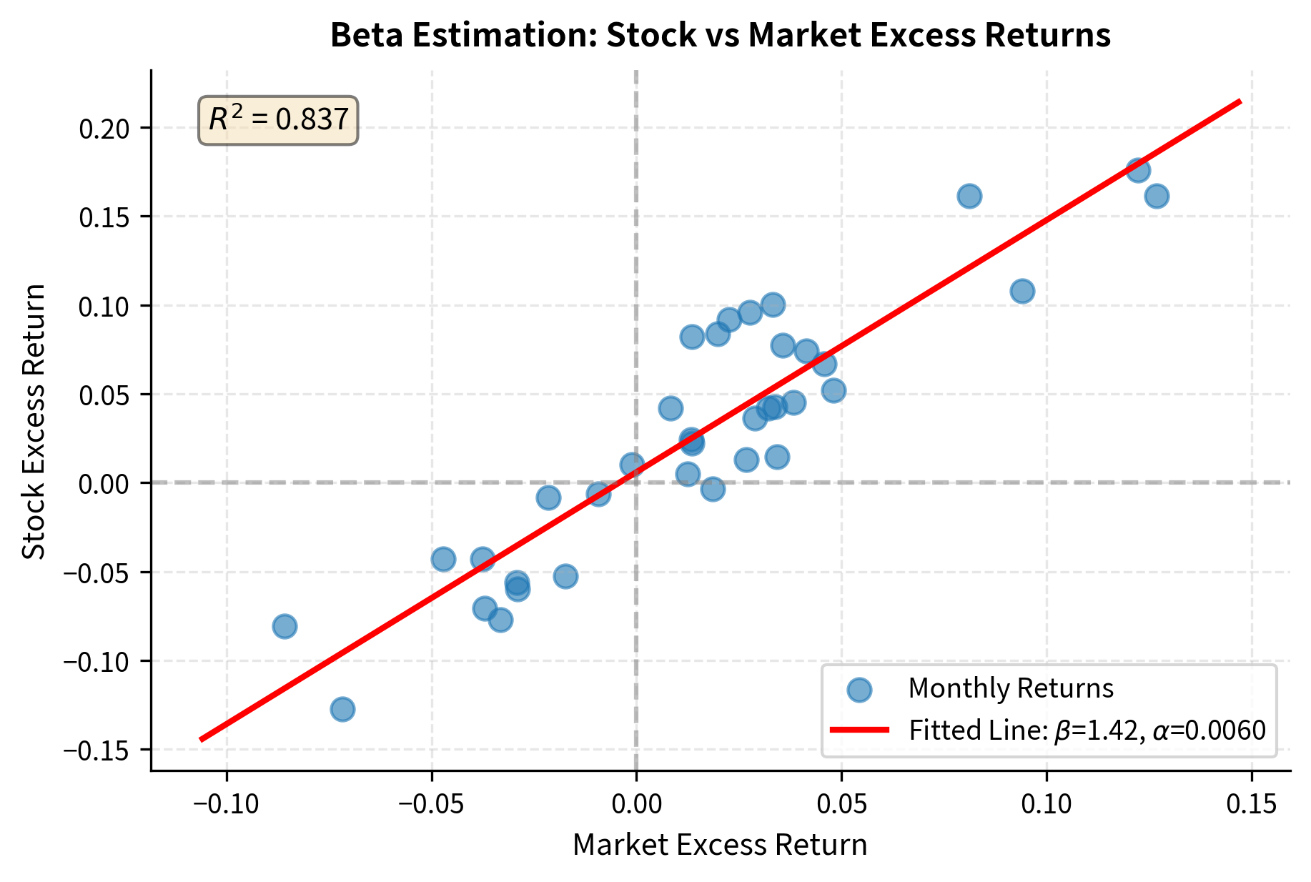
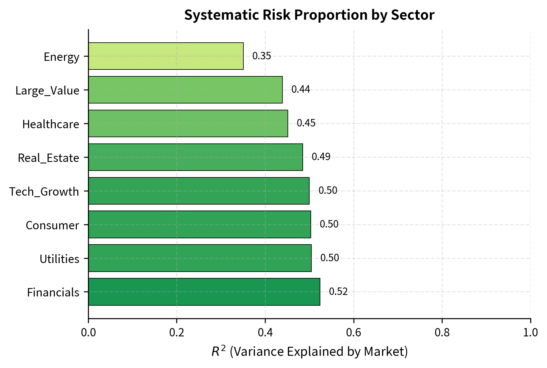
The R-squared value indicates how much of the stock's variance is explained by market movements. A higher R-squared suggests more systematic risk relative to idiosyncratic risk. For well-diversified portfolios, R-squared approaches 1.0 because idiosyncratic risks cancel out. For individual stocks, values typically range from 0.2 to 0.5, indicating that most of a single stock's volatility comes from firm-specific factors rather than market movements. This observation reinforces why diversification matters: individual stocks are driven largely by idiosyncratic factors that can be eliminated through portfolio construction.

Complete CAPM ImplementationLink Copied

Let's bring together the concepts from this chapter in a comprehensive implementation that estimates betas, constructs the Security Market Line, and calculates portfolio alphas. This implementation demonstrates how the theoretical framework translates into practical analysis tools.

In[21]:

Code

import numpy as np
from scipy import stats


class CAPMAnalysis:
    """
    Complete CAPM analysis toolkit for portfolio and security analysis.
    """

    def __init__(self, returns_df, market_returns, rf_rate):
        """
        Initialize with return data.

        Parameters:
        -----------
        returns_df : pd.DataFrame
            Asset returns with assets as columns
        market_returns : pd.Series
            Market index returns
        rf_rate : float
            Risk-free rate (same frequency as returns)
        """
        self.returns = returns_df
        self.market_returns = market_returns
        self.rf = rf_rate
        self.excess_returns = returns_df.subtract(rf_rate, axis=0)
        self.market_excess = market_returns - rf_rate
        self.betas = {}
        self.alphas = {}
        self.r_squared = {}

    def estimate_betas(self):
        """Estimate beta for each asset using OLS regression."""
        for asset in self.returns.columns:
            slope, intercept, r_value, _, _ = stats.linregress(
                self.market_excess, self.excess_returns[asset]
            )
            self.betas[asset] = slope
            self.alphas[asset] = intercept
            self.r_squared[asset] = r_value**2
        return self.betas

    def get_capm_expected_return(self, beta):
        """Calculate CAPM expected return for a given beta."""
        market_premium = self.market_returns.mean() - self.rf
        return self.rf + beta * market_premium

    def security_market_line(self, beta_range=None):
        """Generate Security Market Line data."""
        if beta_range is None:
            beta_range = np.linspace(0, 2, 100)
        market_premium = self.market_returns.mean() - self.rf
        expected_returns = self.rf + beta_range * market_premium
        return beta_range, expected_returns

    def portfolio_beta(self, weights):
        """Calculate portfolio beta as weighted average."""
        if not self.betas:
            self.estimate_betas()
        beta_values = [self.betas[asset] for asset in self.returns.columns]
        return np.dot(weights, beta_values)

    def tracking_error(self, weights, target_beta=1.0):
        """Calculate deviation from target beta."""
        return abs(self.portfolio_beta(weights) - target_beta)

import numpy as np
from scipy import stats


class CAPMAnalysis:
    """
    Complete CAPM analysis toolkit for portfolio and security analysis.
    """

    def __init__(self, returns_df, market_returns, rf_rate):
        """
        Initialize with return data.

        Parameters:
        -----------
        returns_df : pd.DataFrame
            Asset returns with assets as columns
        market_returns : pd.Series
            Market index returns
        rf_rate : float
            Risk-free rate (same frequency as returns)
        """
        self.returns = returns_df
        self.market_returns = market_returns
        self.rf = rf_rate
        self.excess_returns = returns_df.subtract(rf_rate, axis=0)
        self.market_excess = market_returns - rf_rate
        self.betas = {}
        self.alphas = {}
        self.r_squared = {}

    def estimate_betas(self):
        """Estimate beta for each asset using OLS regression."""
        for asset in self.returns.columns:
            slope, intercept, r_value, _, _ = stats.linregress(
                self.market_excess, self.excess_returns[asset]
            )
            self.betas[asset] = slope
            self.alphas[asset] = intercept
            self.r_squared[asset] = r_value**2
        return self.betas

    def get_capm_expected_return(self, beta):
        """Calculate CAPM expected return for a given beta."""
        market_premium = self.market_returns.mean() - self.rf
        return self.rf + beta * market_premium

    def security_market_line(self, beta_range=None):
        """Generate Security Market Line data."""
        if beta_range is None:
            beta_range = np.linspace(0, 2, 100)
        market_premium = self.market_returns.mean() - self.rf
        expected_returns = self.rf + beta_range * market_premium
        return beta_range, expected_returns

    def portfolio_beta(self, weights):
        """Calculate portfolio beta as weighted average."""
        if not self.betas:
            self.estimate_betas()
        beta_values = [self.betas[asset] for asset in self.returns.columns]
        return np.dot(weights, beta_values)

    def tracking_error(self, weights, target_beta=1.0):
        """Calculate deviation from target beta."""
        return abs(self.portfolio_beta(weights) - target_beta)

With the CAPMAnalysis class defined, we generate a synthetic dataset representing different sectors to demonstrate the workflow. The simulation creates returns that follow the CAPM structure, with each sector having a distinct beta and alpha reflecting its risk characteristics and potential mispricing.

In[22]:

Code

# Generate realistic simulated data for demonstration
np.random.seed(2024)
n_periods_full = 60  # 5 years monthly

# Market returns
market_ret = np.random.normal(0.008, 0.04, n_periods_full)

# Asset characteristics
assets = {
    "Tech_Growth": {"beta": 1.4, "alpha": 0.003, "idio_vol": 0.06},
    "Large_Value": {"beta": 0.9, "alpha": 0.001, "idio_vol": 0.03},
    "Utilities": {"beta": 0.5, "alpha": 0.0005, "idio_vol": 0.02},
    "Healthcare": {"beta": 0.7, "alpha": 0.002, "idio_vol": 0.035},
    "Financials": {"beta": 1.2, "alpha": -0.001, "idio_vol": 0.05},
    "Consumer": {"beta": 0.85, "alpha": 0.0015, "idio_vol": 0.03},
    "Energy": {"beta": 1.1, "alpha": -0.002, "idio_vol": 0.055},
    "Real_Estate": {"beta": 0.95, "alpha": 0.001, "idio_vol": 0.04},
}

rf_monthly = 0.003  # ~3.6% annual

# Generate returns
returns_data = {}
for name, params in assets.items():
    idio = np.random.normal(0, params["idio_vol"], n_periods_full)
    returns_data[name] = (
        rf_monthly
        + params["alpha"]
        + params["beta"] * (market_ret - rf_monthly)
        + idio
    )

returns_df = pd.DataFrame(returns_data)
market_series = pd.Series(market_ret, name="Market")

# Generate realistic simulated data for demonstration
np.random.seed(2024)
n_periods_full = 60  # 5 years monthly

# Market returns
market_ret = np.random.normal(0.008, 0.04, n_periods_full)

# Asset characteristics
assets = {
    "Tech_Growth": {"beta": 1.4, "alpha": 0.003, "idio_vol": 0.06},
    "Large_Value": {"beta": 0.9, "alpha": 0.001, "idio_vol": 0.03},
    "Utilities": {"beta": 0.5, "alpha": 0.0005, "idio_vol": 0.02},
    "Healthcare": {"beta": 0.7, "alpha": 0.002, "idio_vol": 0.035},
    "Financials": {"beta": 1.2, "alpha": -0.001, "idio_vol": 0.05},
    "Consumer": {"beta": 0.85, "alpha": 0.0015, "idio_vol": 0.03},
    "Energy": {"beta": 1.1, "alpha": -0.002, "idio_vol": 0.055},
    "Real_Estate": {"beta": 0.95, "alpha": 0.001, "idio_vol": 0.04},
}

rf_monthly = 0.003  # ~3.6% annual

# Generate returns
returns_data = {}
for name, params in assets.items():
    idio = np.random.normal(0, params["idio_vol"], n_periods_full)
    returns_data[name] = (
        rf_monthly
        + params["alpha"]
        + params["beta"] * (market_ret - rf_monthly)
        + idio
    )

returns_df = pd.DataFrame(returns_data)
market_series = pd.Series(market_ret, name="Market")

We initialize the analysis with our returns data and estimate the beta for each asset. The estimation process runs separate regressions for each sector, extracting the slope coefficient as the beta estimate.

In[23]:

Code

# Run CAPM analysis
capm = CAPMAnalysis(returns_df, market_series, rf_monthly)
capm.estimate_betas()

# Create summary DataFrame
summary_data = []
for asset in returns_df.columns:
    actual_ret = returns_df[asset].mean()
    expected_ret = capm.get_capm_expected_return(capm.betas[asset])
    summary_data.append(
        {
            "Asset": asset,
            "Beta": capm.betas[asset],
            "R²": capm.r_squared[asset],
            "Actual Return": actual_ret * 12,  # Annualized
            "CAPM Expected": expected_ret * 12,  # Annualized
            "Alpha (Annual)": capm.alphas[asset] * 12,
        }
    )

summary_df = pd.DataFrame(summary_data)

# Run CAPM analysis
capm = CAPMAnalysis(returns_df, market_series, rf_monthly)
capm.estimate_betas()

# Create summary DataFrame
summary_data = []
for asset in returns_df.columns:
    actual_ret = returns_df[asset].mean()
    expected_ret = capm.get_capm_expected_return(capm.betas[asset])
    summary_data.append(
        {
            "Asset": asset,
            "Beta": capm.betas[asset],
            "R²": capm.r_squared[asset],
            "Actual Return": actual_ret * 12,  # Annualized
            "CAPM Expected": expected_ret * 12,  # Annualized
            "Alpha (Annual)": capm.alphas[asset] * 12,
        }
    )

summary_df = pd.DataFrame(summary_data)

Finally, we display the summary statistics to compare the actual and expected returns.

Out[24]:

Console

CAPM Analysis Summary
=====================================================================================
      Asset  Beta    R²  Actual Return  CAPM Expected  Alpha (Annual)
Tech_Growth 1.516 0.500          0.164          0.170          -0.006
Large_Value 0.755 0.439          0.196          0.103           0.093
  Utilities 0.539 0.504          0.054          0.084          -0.030
 Healthcare 0.843 0.451         -0.008          0.111          -0.119
 Financials 1.351 0.524          0.112          0.156          -0.044
   Consumer 0.870 0.503          0.156          0.113           0.043
     Energy 1.208 0.351          0.062          0.143          -0.081
Real_Estate 1.087 0.485          0.169          0.132           0.037

The summary table displays the key metrics for each asset. 'Tech_Growth' and 'Financials' exhibit betas above 1.0, indicating they carry more systematic risk than the market. Conversely, 'Utilities' has a beta of 0.5, confirming its defensive nature. The alpha values show the divergence between actual and expected returns; positive alphas suggest potential undervaluation or superior performance adjusted for risk. The R-squared values indicate how much of each sector's return variation is explained by market movements, with higher values suggesting greater systematic risk exposure relative to idiosyncratic risk.

We can also visualize these results on the Security Market Line to see the alphas graphically.

Out[25]:

Visualization

Scatter plot of assets showing beta versus expected return with Security Market Line. — Complete CAPM analysis visualizing asset returns against the Security Market Line (SML). High-beta sectors like 'Tech_Growth' and 'Financials' appear on the right, while defensive 'Utilities' appear on the left. Vertical deviations from the SML reveal alpha, with 'Healthcare' showing positive alpha (outperformance) and 'Energy' showing negative alpha (underperformance).

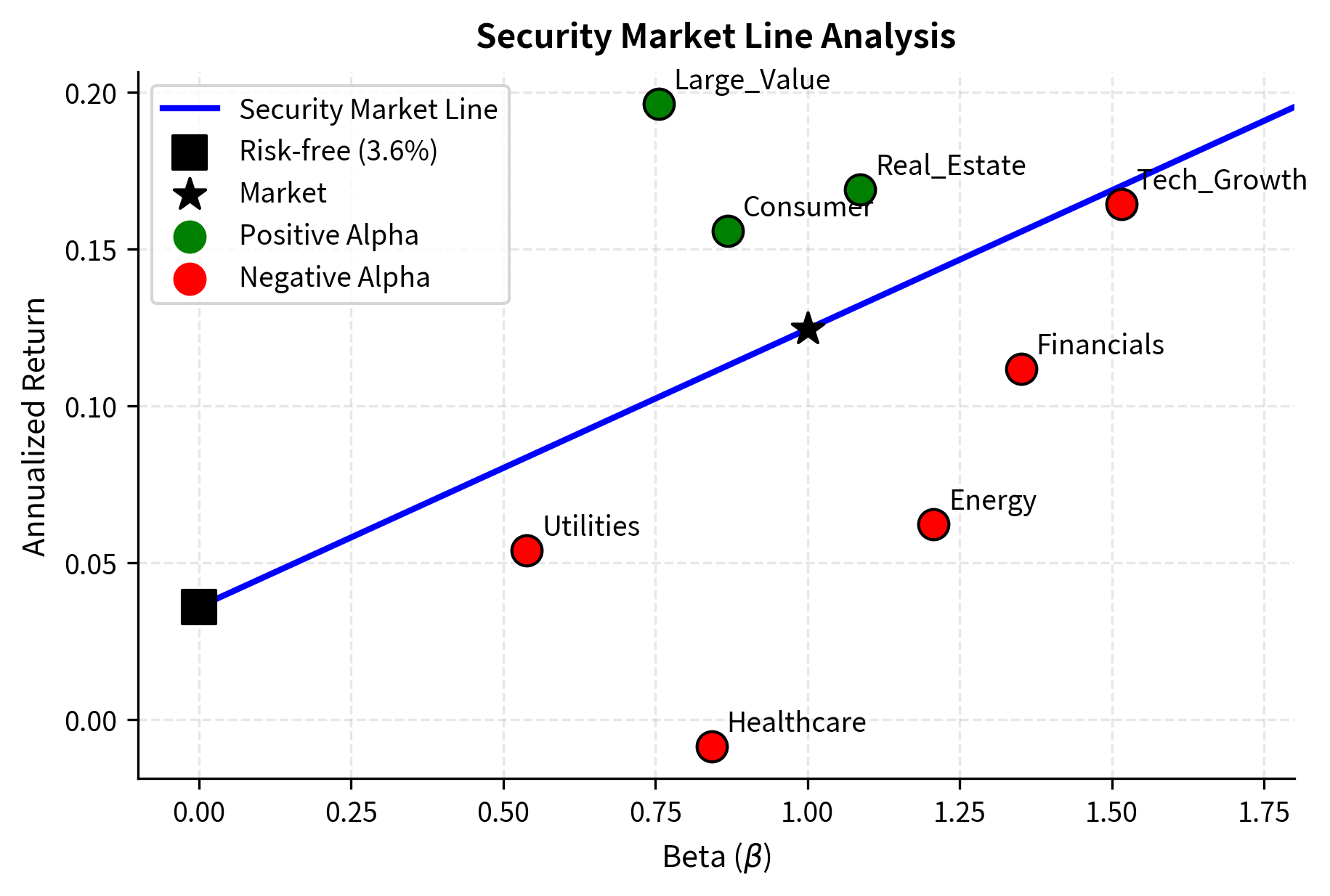
The analysis reveals several patterns consistent with CAPM theory. Higher-beta assets like Tech_Growth and Financials show higher expected returns, while defensive sectors like Utilities exhibit lower betas and returns. The spread of assets around the SML represents alpha, either skill/mispricing or compensation for risks not captured by CAPM. This visualization makes it easy to identify which sectors are outperforming or underperforming their risk-adjusted benchmarks, providing actionable insights for portfolio construction.

The R-squared values from our CAPM analysis reveal how much of each sector's return variation is explained by market movements. We can visualize these values to compare systematic versus idiosyncratic risk across sectors.

Out[26]:

Visualization

Bar chart showing R-squared values for different sectors from CAPM regression. — R-squared values across sectors show the proportion of return variance explained by market movements. Higher R-squared indicates greater systematic risk exposure, while lower values suggest more idiosyncratic risk that can be diversified away.

Key ParametersLink Copied

The key parameters for the CAPM implementation are:

returns: Historical asset returns used to estimate beta and alpha.
market_returns: Returns of the broad market index (e.g., S&P 500) used as the systematic risk factor.
rf: Risk-free rate of return, used to calculate excess returns for both assets and the market.
beta (β): Measure of systematic risk, calculated as the slope of the regression of asset excess returns on market excess returns.
alpha (α): Measure of abnormal return, calculated as the intercept of the regression.

Limitations and Empirical ChallengesLink Copied

Despite its theoretical elegance, CAPM has faced significant empirical challenges since its development. Understanding these limitations is crucial for you.

The Market Portfolio ProblemLink Copied

CAPM's central prediction involves the market portfolio, but this portfolio is inherently unobservable. It should include all investable assets globally: stocks, bonds, real estate, commodities, art, human capital, and more. Richard Roll's critique, published in 1977, argued that CAPM is essentially untestable because any test uses a proxy (like the S&P 500) that differs from the true market portfolio. A rejection of CAPM using a proxy may simply indicate that the proxy is inefficient, not that the theory is wrong.

Empirical AnomaliesLink Copied

Decades of empirical research have identified systematic patterns in returns that CAPM fails to explain:

Size effect: Small-cap stocks have historically earned higher returns than large-cap stocks, even after adjusting for their higher betas. This anomaly was documented by Rolf Banz in 1981 and has persisted across markets and time periods, though it has weakened in recent decades.
Value effect: Stocks with high book-to-market ratios (value stocks) have outperformed stocks with low book-to-market ratios (growth stocks), controlling for beta. Eugene Fama and Kenneth French documented this extensively, leading to their famous three-factor model, which we'll explore in the next chapter on Arbitrage Pricing Theory and Multi-Factor Models.
Momentum effect: Stocks that have performed well over the past 3-12 months tend to continue outperforming, while recent losers continue underperforming. This effect, documented by Jegadeesh and Titman (1993), contradicts the efficient market hypothesis implicit in CAPM.
Low-volatility anomaly: Contrary to CAPM's prediction that higher risk should command higher returns, low-volatility stocks have historically outperformed high-volatility stocks on a risk-adjusted basis. This challenges the fundamental risk-return tradeoff at the heart of the model.

Beta InstabilityLink Copied

Beta estimates are unstable over time. A stock's beta can change significantly as the company's business evolves, financial leverage changes, or market conditions shift. This instability creates challenges for forward-looking applications:

In[27]:

Code

import numpy as np
from scipy import stats

# Demonstrate beta instability over rolling windows
np.random.seed(303)
n_periods_long = 120  # 10 years monthly

# True beta that changes over time
true_beta_path = np.concatenate(
    [
        np.ones(30) * 0.8,  # First 2.5 years: defensive
        np.ones(30) * 1.4,  # Next 2.5 years: aggressive after acquisition
        np.ones(30) * 1.1,  # Next 2.5 years: normalizing
        np.ones(30) * 0.9,  # Final 2.5 years: mature company
    ]
)

market_long = np.random.normal(0.007, 0.04, n_periods_long)
stock_long = np.array(
    [
        true_beta_path[i] * market_long[i] + np.random.normal(0, 0.03)
        for i in range(n_periods_long)
    ]
)

# Rolling beta estimation (36-month window)
window = 36
rolling_betas = []
rolling_dates = list(range(window, n_periods_long + 1))

for end in rolling_dates:
    start = end - window
    slope, _, _, _, _ = stats.linregress(
        market_long[start:end], stock_long[start:end]
    )
    rolling_betas.append(slope)

import numpy as np
from scipy import stats

# Demonstrate beta instability over rolling windows
np.random.seed(303)
n_periods_long = 120  # 10 years monthly

# True beta that changes over time
true_beta_path = np.concatenate(
    [
        np.ones(30) * 0.8,  # First 2.5 years: defensive
        np.ones(30) * 1.4,  # Next 2.5 years: aggressive after acquisition
        np.ones(30) * 1.1,  # Next 2.5 years: normalizing
        np.ones(30) * 0.9,  # Final 2.5 years: mature company
    ]
)

market_long = np.random.normal(0.007, 0.04, n_periods_long)
stock_long = np.array(
    [
        true_beta_path[i] * market_long[i] + np.random.normal(0, 0.03)
        for i in range(n_periods_long)
    ]
)

# Rolling beta estimation (36-month window)
window = 36
rolling_betas = []
rolling_dates = list(range(window, n_periods_long + 1))

for end in rolling_dates:
    start = end - window
    slope, _, _, _, _ = stats.linregress(
        market_long[start:end], stock_long[start:end]
    )
    rolling_betas.append(slope)

We plot the estimated beta over time against the true beta to observe the lag and instability.

Out[28]:

Visualization

Line chart comparing estimated rolling beta to true beta over time showing instability. — Comparison of true beta (dashed red) and estimated rolling 36-month beta (blue) over time. The estimated beta lags the true structural changes in the company's risk profile, illustrating the delay inherent in historical beta estimation methods.

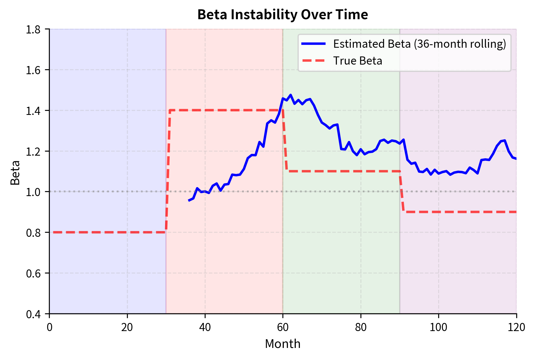
The figure illustrates how rolling beta estimates lag changes in true beta due to the historical estimation window. When making forward-looking decisions, we must decide whether historical beta represents future risk exposure.

Model ExtensionsLink Copied

The empirical failures of CAPM led to important extensions:

Multi-factor models: Rather than a single market factor, these models include additional factors (size, value, momentum, quality) that help explain cross-sectional return differences. The Fama-French three-factor and five-factor models are widely used alternatives, which we'll cover in the next chapter.
Conditional CAPM: Time-varying betas and risk premiums can capture changing market conditions. Beta might be higher during recessions when correlations increase.
Consumption CAPM: Replacing market returns with consumption growth provides a stronger theoretical foundation but faces its own empirical challenges.

Despite these limitations, CAPM remains valuable as a benchmark model, a way to decompose returns into systematic and idiosyncratic components, and a framework for thinking about risk and return relationships. Its simplicity makes it a practical tool even when more sophisticated models are available.

SummaryLink Copied

This chapter introduced the Capital Asset Pricing Model, which extends modern portfolio theory to derive equilibrium asset prices. The key insights and concepts include:

The introduction of a risk-free asset transforms the efficient frontier from a curve into a straight line, the Capital Market Line (CML). All mean-variance investors combine the risk-free asset with the same tangency portfolio, which in equilibrium must be the market portfolio.

Systematic risk is the only risk that commands a premium in the market. Unsystematic (idiosyncratic) risk can be diversified away at no cost, so you should not expect compensation for bearing it. This insight is foundational for understanding how assets should be priced.

Beta measures an asset's systematic risk, its sensitivity to market movements. It captures how much an asset's return is expected to change for a 1% change in the market return. Beta is estimated through regression analysis and exhibits instability over time.

The Security Market Line (SML) describes the equilibrium relationship between expected return and beta for all assets: $E[R_i] = R_f + \beta_i(E[R_M] - R_f)$ . This is the CAPM equation, the model's central prediction.

Alpha measures performance beyond what CAPM predicts. Positive alpha indicates outperformance after adjusting for systematic risk. Generating persistent positive alpha is the goal of active investment management, though distinguishing skill from luck remains challenging.

CAPM faces significant empirical challenges, including the size effect, value effect, momentum, and the low-volatility anomaly. These failures motivated the development of multi-factor models. Nevertheless, CAPM provides a crucial framework for understanding risk-return relationships and serves as the benchmark for evaluating investment performance.

In the next chapter, we'll explore Arbitrage Pricing Theory and multi-factor models, which address some of CAPM's limitations by allowing multiple sources of systematic risk.

QuizLink Copied

Ready to test your understanding? Take this quick quiz to reinforce what you've learned about the Capital Asset Pricing Model and the efficient frontier.

Loading component...

Comments

Back to Quantitative Finance

Previous Chapter

Modern Portfolio Theory and Mean-Variance Optimization

Next Chapter

Arbitrage Pricing Theory and Multi-Factor Models

Reference

BIBTEXAcademic

@misc{capitalassetpricingmodelbetaalphasystematicrisk, author = {Michael Brenndoerfer}, title = {Capital Asset Pricing Model: Beta, Alpha & Systematic Risk}, year = {2025}, url = {https://mbrenndoerfer.com/writing/capm-capital-asset-pricing-model-beta-systematic-risk}, organization = {mbrenndoerfer.com}, note = {Accessed: 2025-01-01} }

APAAcademic

Michael Brenndoerfer (2025). Capital Asset Pricing Model: Beta, Alpha & Systematic Risk. Retrieved from https://mbrenndoerfer.com/writing/capm-capital-asset-pricing-model-beta-systematic-risk

MLAAcademic

Michael Brenndoerfer. "Capital Asset Pricing Model: Beta, Alpha & Systematic Risk." 2026. Web. today. <https://mbrenndoerfer.com/writing/capm-capital-asset-pricing-model-beta-systematic-risk>.

CHICAGOAcademic

Michael Brenndoerfer. "Capital Asset Pricing Model: Beta, Alpha & Systematic Risk." Accessed today. https://mbrenndoerfer.com/writing/capm-capital-asset-pricing-model-beta-systematic-risk.

HARVARDAcademic

Michael Brenndoerfer (2025) 'Capital Asset Pricing Model: Beta, Alpha & Systematic Risk'. Available at: https://mbrenndoerfer.com/writing/capm-capital-asset-pricing-model-beta-systematic-risk (Accessed: today).

SimpleBasic

Michael Brenndoerfer (2025). Capital Asset Pricing Model: Beta, Alpha & Systematic Risk. https://mbrenndoerfer.com/writing/capm-capital-asset-pricing-model-beta-systematic-risk

Direct link:

https://mbrenndoerfer.com/writing/capm-capital-asset-pricing-model-beta-systematic-risk

About the author: Michael Brenndoerfer

All opinions expressed here are my own and do not reflect the views of my employer.

Michael currently works as an Associate Director of Data Science at EQT Partners in Singapore, leading AI and data initiatives across private capital investments.

With over a decade of experience spanning private equity, management consulting, and software engineering, he specializes in building and scaling analytics capabilities from the ground up. He has published research in leading AI conferences and holds expertise in machine learning, natural language processing, and value creation through data.

View Full Resume Publications Contact Books

Capital Asset Pricing Model: Beta, Alpha & Systematic Risk

Capital Market Theory: CAPM and the Efficient FrontierLink Copied

Assumptions of CAPMLink Copied

The Risk-Free Asset and Portfolio CombinationsLink Copied

The Capital Market Line and Market PortfolioLink Copied

Systematic and Unsystematic RiskLink Copied

Beta: The Measure of Systematic RiskLink Copied

The Security Market LineLink Copied

Alpha: Measuring Abnormal ReturnsLink Copied

Estimating Beta in PracticeLink Copied

Complete CAPM ImplementationLink Copied

Key ParametersLink Copied

Limitations and Empirical ChallengesLink Copied

The Market Portfolio ProblemLink Copied

Empirical AnomaliesLink Copied

Beta InstabilityLink Copied

Model ExtensionsLink Copied

SummaryLink Copied

QuizLink Copied

Comments

Reference

About the author: Michael Brenndoerfer

Related Content

Advanced Portfolio Construction: Black-Litterman & Risk Parity

Performance Attribution: Measuring Alpha and Beta Sources

Portfolio Performance Measurement: Risk-Adjusted Returns & Drawdown Analysis

Stay updated

Comments

About the author: Michael Brenndoerfer

Related Content

Advanced Portfolio Construction: Black-Litterman & Risk Parity

Performance Attribution: Measuring Alpha and Beta Sources

Portfolio Performance Measurement: Risk-Adjusted Returns & Drawdown Analysis

Stay updated