

Learn Modern Portfolio Theory and mean-variance optimization. Master the efficient frontier, diversification mathematics, and optimal portfolio construction.
Choose your expertise level to adjust how many terms are explained. Beginners see more tooltips, experts see fewer to maintain reading flow. Hover over underlined terms for instant definitions.
Modern Portfolio Theory and Mean-Variance Optimization
In 1952, Harry Markowitz published a paper titled "Portfolio Selection" that fundamentally changed how investors think about risk and return. Before Markowitz, investment analysis focused almost exclusively on picking individual securities with the best expected returns. Markowitz introduced a revolutionary insight: the risk of a portfolio depends not just on the risks of individual assets, but critically on how those assets move together. This observation gave birth to Modern Portfolio Theory (MPT) and provided the first rigorous mathematical framework for constructing optimal portfolios.
The core idea is straightforward. Investors care about two things: maximizing expected return and minimizing risk. Markowitz formalized risk as the variance (or standard deviation) of portfolio returns, creating what we now call the mean-variance framework. Within this framework, rational investors should only hold portfolios that offer the highest expected return for a given level of risk, or equivalently, the lowest risk for a given expected return. These optimal portfolios form the efficient frontier, a concept that remains central to investment management today.
This chapter develops the mathematical machinery of mean-variance optimization from first principles. We'll see how diversification arises naturally from the mathematics of combining assets with less-than-perfect correlation, and we'll implement practical algorithms for finding optimal portfolios. The framework we develop here provides the foundation for the Capital Asset Pricing Model and factor models that follow in subsequent chapters.
Portfolio Returns and Risk
Before we can optimize portfolios, we need precise definitions of portfolio return and risk. These definitions form the foundation for Modern Portfolio Theory. We need accurate measures of portfolio return and risk to compare investment strategies and identify optimal allocations.
Suppose we allocate wealth across assets. The fundamental question is: how should we combine individual asset characteristics to describe the portfolio as a whole? Let denote the fraction of wealth invested in asset , where the weights must sum to one:
where:
- : fraction of wealth invested in asset
- : total number of assets in the portfolio
This constraint ensures we account for all invested capital. A weight of 0.3 means 30% of the portfolio is allocated to that asset. We allow short selling, meaning weights can be negative (representing borrowed positions). Shorting an asset involves selling borrowed shares with the obligation to return them later, creating a negative position that profits when the price falls.
Expected Portfolio Return
The expected return of a portfolio follows naturally from the linearity of expectation, a concept we explored in our probability foundations. If each asset has expected return , the portfolio's expected return is simply the weighted average:
where:
- : expected return of the portfolio
- : expected value of portfolio return
- : weight of asset
- : expected return of asset
- : vector of portfolio weights,
- : vector of expected returns,
This formula tells us something intuitive: a portfolio's expected return is determined entirely by how much we invest in each asset and what return we expect from that asset. There are no interaction effects or nonlinearities. If we double our allocation to a high-return asset, we increase the portfolio's expected return proportionally. Vector notation provides a compact way to represent many assets.
Portfolio Variance
The portfolio variance requires more care and reveals how diversification works mathematically. Unlike expected return, variance does not simply average across assets. The portfolio return is:
where:
- : return of the portfolio
- : weight of asset
- : return of asset
- : number of assets
To find the variance of this weighted sum, we must account for how each pair of assets moves together. Taking the variance and using the linearity properties we covered in Part I:
where:
- : variance of the portfolio
- : weights allocated to assets and
- : covariance between returns of assets and
The double summation captures all pairwise interactions between assets. When , the covariance term becomes the variance of asset , contributing to portfolio variance. When , the covariance measures how assets and move together, and this is where diversification benefits emerge.
Let denote the covariance matrix, where . Then the portfolio variance is:
where:
- : variance of the portfolio
- : vector of portfolio weights
- : covariance matrix of asset returns
This compact matrix notation, which we developed in Part I's linear algebra chapter, makes optimization tractable. The quadratic form appears throughout financial mathematics because it elegantly encapsulates how portfolio risk depends on both individual asset volatilities (the diagonal of ) and their correlations (the off-diagonal elements).
The covariance matrix is symmetric () and positive semi-definite, meaning for all weight vectors . This ensures portfolio variance is always non-negative. When is positive definite, the portfolio variance is strictly positive for any non-trivial portfolio.
The Two-Asset Case
The two-asset case provides crucial intuition before we tackle the general problem. By working through this simplified scenario, we can develop a geometric understanding of how risk and return interact, seeing clearly how correlation shapes the set of achievable portfolios. Consider a portfolio with weights in asset 1 and in asset 2.
The expected return is:
where:
- : expected return of the portfolio
- : weight invested in asset 1
- : expected returns of assets 1 and 2
This formula shows that expected return varies linearly with the weight . As we shift allocation from asset 2 toward asset 1, expected return moves along a straight line between (when ) and (when ). There are no surprises here: return blending is straightforward.
The variance, however, tells a richer story:
where:
- : variance of the portfolio
- : weight invested in asset 1
- : standard deviations (volatility) of assets 1 and 2
- : correlation coefficient between returns of assets 1 and 2
This equation has three terms, each revealing a different aspect of portfolio risk. The first term, , captures the contribution of asset 1's own volatility, scaled by the square of its weight. The second term, , does the same for asset 2. The third term, the cross-term , is where the diversification benefit arises. This term depends on the correlation , and its sign and magnitude determine whether combining the two assets reduces or amplifies total portfolio risk.
The Diversification Effect
The diversification effect emerges from this variance formula. Consider what happens when . The cross-term is smaller than it would be under perfect correlation, reducing total portfolio variance. When correlation is negative, this term actually becomes negative, further reducing portfolio risk below what the individual variances would suggest.
To understand this intuitively, imagine two assets that tend to move in opposite directions. When one zigs, the other zags. In a portfolio containing both, these opposite movements partially cancel each other, smoothing the overall portfolio return and reducing its volatility. The lower the correlation, the more pronounced this cancellation effect.
Let's see this numerically:
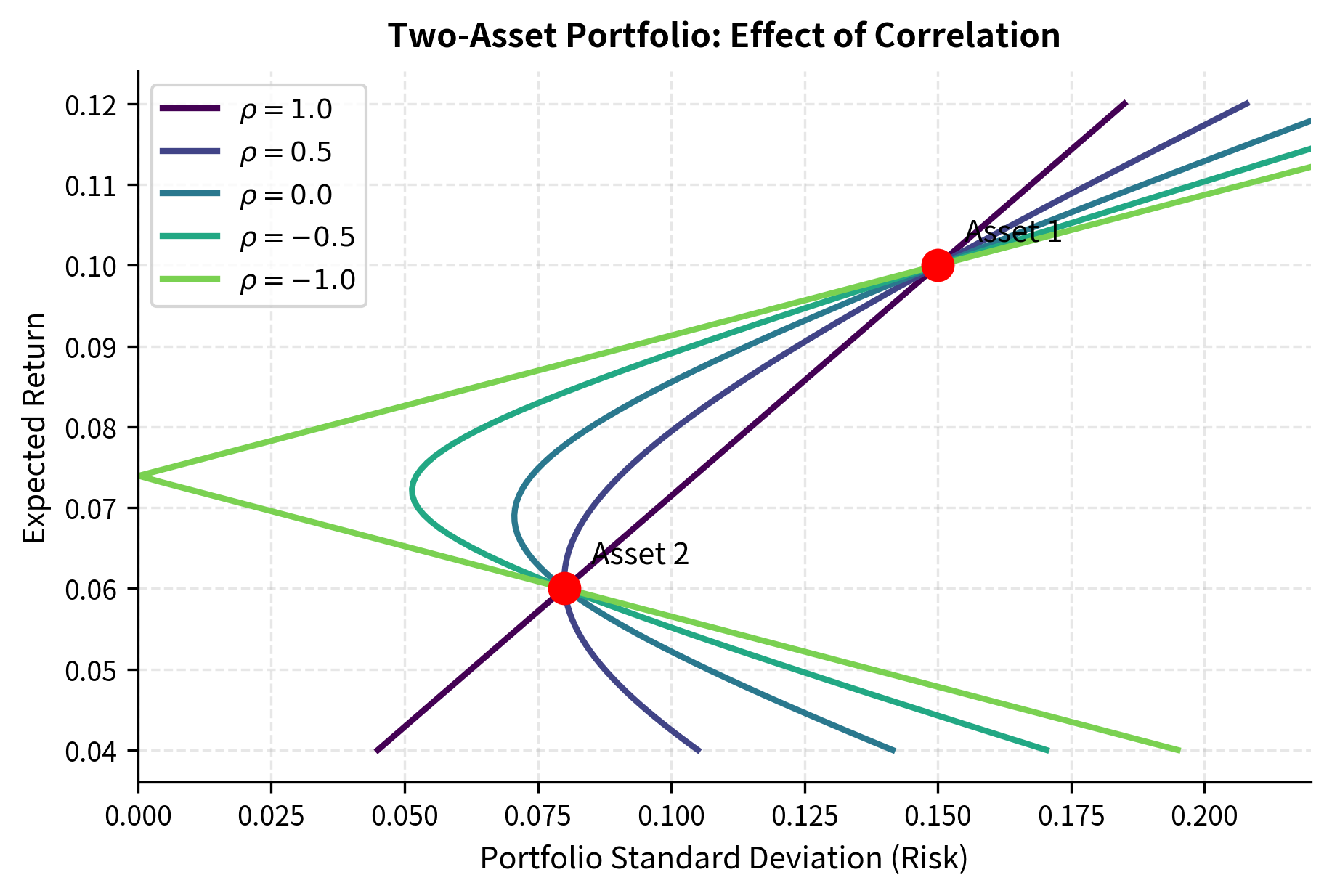
The figure reveals several key insights about how correlation shapes investment opportunities:
- Perfect positive correlation (\rho = 1): The frontier is a straight line. Diversification provides no risk reduction; portfolio risk is simply the weighted average of individual risks. The two assets move in perfect lockstep, so combining them cannot smooth out volatility.
- Imperfect correlation (): The frontier curves leftward, meaning some portfolios achieve lower risk than either asset alone. This is the diversification benefit. The curvature increases as correlation decreases, opening up more favorable risk-return combinations.
- Perfect negative correlation (): A risk-free portfolio exists. When , the portfolio variance is exactly zero. This extreme case illustrates the theoretical maximum of diversification: if two assets move in perfectly opposite directions, we can combine them to eliminate all uncertainty.
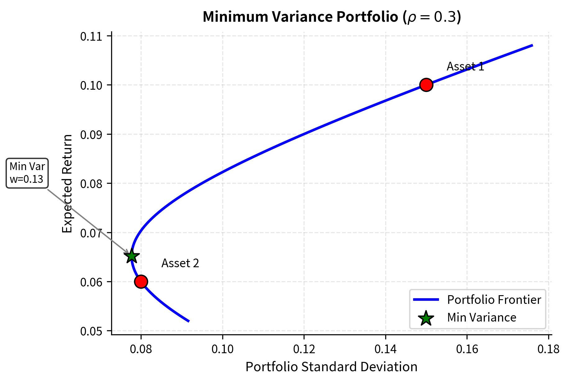
Minimum Variance Portfolio
For the two-asset case, we can find the minimum variance portfolio analytically. This portfolio represents the allocation that achieves the lowest possible risk, regardless of the expected return it delivers. To find the minimum variance portfolio, we differentiate the variance with respect to and set the result to zero:
The derivative includes three components corresponding to the three terms in the variance formula. Setting this derivative to zero identifies the point where small changes in produce no change in variance, which is precisely the minimum. Rearranging the first-order condition to isolate :
Solving for :
where:
- : optimal weight for asset 1 to minimize portfolio variance
- : volatilities of assets 1 and 2
- : correlation between assets 1 and 2
This formula balances the volatilities and correlation to minimize risk. If the assets are uncorrelated (), the weight is proportional to , meaning the portfolio holds more of the asset with lower volatility. This makes intuitive sense: when assets don't interact, we should tilt toward the less risky one. As correlation decreases (becomes more negative), the optimal weight shifts to exploit the hedging benefit, potentially allocating more to the higher-volatility asset because its movements offset those of the other asset.
The minimum variance portfolio achieves lower risk than either individual asset. This is the fundamental benefit of diversification. Even though both assets carry uncertainty, combining them in the right proportions produces a portfolio with less uncertainty than holding either one alone. This result, sometimes called the "free lunch" of diversification, arises purely from the mathematics of combining imperfectly correlated random variables.
Multi-Asset Portfolio Optimization
With more than two assets, we need the full matrix formulation. The principles remain the same, but the algebra becomes more complex, requiring linear algebra tools to express and solve the optimization problem efficiently. Let be the vector of weights, the vector of expected returns, and the covariance matrix.
The optimization problem has two equivalent formulations, each emphasizing a different perspective on the objective:
Formulation 1: Minimize risk for a target return
This formulation starts with a desired level of expected return and asks: what is the least risky way to achieve it?
where:
- : vector of portfolio weights
- : covariance matrix of asset returns
- : vector of expected returns
- : required level of expected return
- : vector of ones (sum constraint)
The factor of in the objective is a mathematical convenience that simplifies the derivatives. It does not change the optimal solution because multiplying an objective by a positive constant does not alter which portfolio minimizes it.
Formulation 2: Maximize utility (mean-variance utility)
This formulation takes a different approach, directly modeling investor preferences through a utility function that trades off return against risk:
where:
- : risk aversion parameter ()
- : vector of portfolio weights
- : vector of expected returns
- : covariance matrix of asset returns
- : vector of ones
The parameter captures how much you dislike risk. If you are highly risk-averse (large ), you penalize variance heavily and will choose a conservative, low-volatility portfolio. If you are risk-tolerant (small ), you care more about expected return and will accept higher volatility to chase higher gains. Both formulations trace out the same efficient frontier; they simply parameterize it differently.
Analytical Solution: Lagrangian Approach
For the first formulation, we form the Lagrangian using the techniques from Part I. The Lagrangian method converts a constrained optimization problem into an unconstrained one by introducing penalty terms for violating constraints:
where:
- : the Lagrangian function
- : vector of portfolio weights
- : covariance matrix of asset returns
- : Lagrange multipliers enforcing the return and budget constraints
- : vector of expected returns
- : target portfolio return
- : vector of ones
The Lagrange multipliers and act as shadow prices, measuring how much the optimal objective would change if we relaxed the corresponding constraint slightly. Taking the derivative with respect to and setting it to zero:
where:
- : covariance matrix
- : vector of portfolio weights
- : Lagrange multipliers
- : vector of expected returns
- : vector of ones
This first-order condition states that at the optimum, the marginal increase in risk from adjusting any weight must be exactly offset by the value of that weight in meeting the return and budget constraints. Rearranging terms to solve for explicitly:
where:
- : optimal portfolio weight vector
- : inverse of the covariance matrix
- : vector of expected returns
- : vector of ones
- : Lagrange multipliers
The formula decomposes the optimal portfolio into two parts: a term proportional to (seeking high returns) and a term proportional to (minimizing variance). The multipliers and weight these components to satisfy the target return and budget constraints. This decomposition reveals the fundamental tension in portfolio construction: the desire for return pulls toward , while the desire for safety pulls toward .
The Lagrange multipliers and are determined by the constraints. Substituting back:
where:
- : target return
- : Lagrange multipliers
- : vector of expected returns
- : inverse covariance matrix
- : vector of ones
These two equations form a linear system in the two unknowns and . We can solve for and in terms of scalar constants derived from the problem parameters:
where:
- : target portfolio return
The constants , , and depend only on the assets' expected returns and covariance structure, not on the target return. This means we can precompute them once and then quickly find optimal portfolios for any target return, making efficient frontier construction computationally efficient.
The Global Minimum Variance Portfolio
Setting (ignoring the return target), we get the global minimum variance (GMV) portfolio:
where:
- : weights of the global minimum variance portfolio
- : inverse of the covariance matrix
- : vector of ones
This formula represents risk minimization in its most basic form. The term identifies the portfolio structure that minimizes variance without regard for expected returns, while the denominator normalizes the weights to sum to one. Assets with lower variance and lower correlation to other assets receive higher weights, as they contribute less to overall portfolio risk.
This portfolio has the lowest possible variance among all portfolios satisfying the budget constraint. It sits at the leftmost point of the efficient frontier, representing the safest allocation available without going to cash. If you care only about minimizing uncertainty (perhaps because you have very short horizons or extreme risk aversion), the GMV portfolio is optimal regardless of expected returns.
The Efficient Frontier
The efficient frontier is the set of all portfolios that offer the maximum expected return for each level of risk. Mathematically, it's the upper boundary of the feasible set in risk-return space. This concept is central to Modern Portfolio Theory because it delineates the best possible tradeoffs available to investors.
To understand the efficient frontier, imagine plotting every possible portfolio in risk-return space. The feasible region, bounded by the budget constraint and any position limits, forms a region. Some portfolios lie on the boundary of this region, while others lie in the interior. Interior portfolios are dominated by boundary portfolios that offer either higher return for the same risk or lower risk for the same return. The efficient frontier consists of all portfolios that are not dominated by any other portfolio.
A portfolio is efficient if no other portfolio offers higher expected return for the same risk, or lower risk for the same expected return. The collection of all efficient portfolios forms the efficient frontier.
Two-Fund Separation Theorem
A remarkable property of mean-variance optimization is the two-fund separation theorem: any efficient portfolio can be expressed as a linear combination of two distinct efficient portfolios. This means efficiency can be achieved regardless of risk preferences by holding different combinations of just two mutual funds.
The theorem significantly affects portfolio management. It suggests that an asset management firm need only offer two efficiently managed funds, and an investor can achieve an optimal portfolio by combining these funds in proportions determined by their risk tolerance. This separation between the "production" of efficient portfolios and your "consumption" choices simplifies the investment process dramatically.
Mathematically, if and are any two efficient portfolios, then for any scalar , the portfolio is also efficient:
where:
- : the new efficient portfolio
- : weighting scalar
- : two distinct efficient portfolios
The parameter determines where along the efficient frontier the combined portfolio sits. When , we hold only portfolio 1; when , we hold only portfolio 2; values between 0 and 1 produce intermediate portfolios. Values outside this range (which require short selling one of the funds) extend the frontier beyond the original two portfolios.
Computing the Frontier
Let's implement efficient frontier computation using quadratic programming:
Worked Example: Three-Asset Portfolio
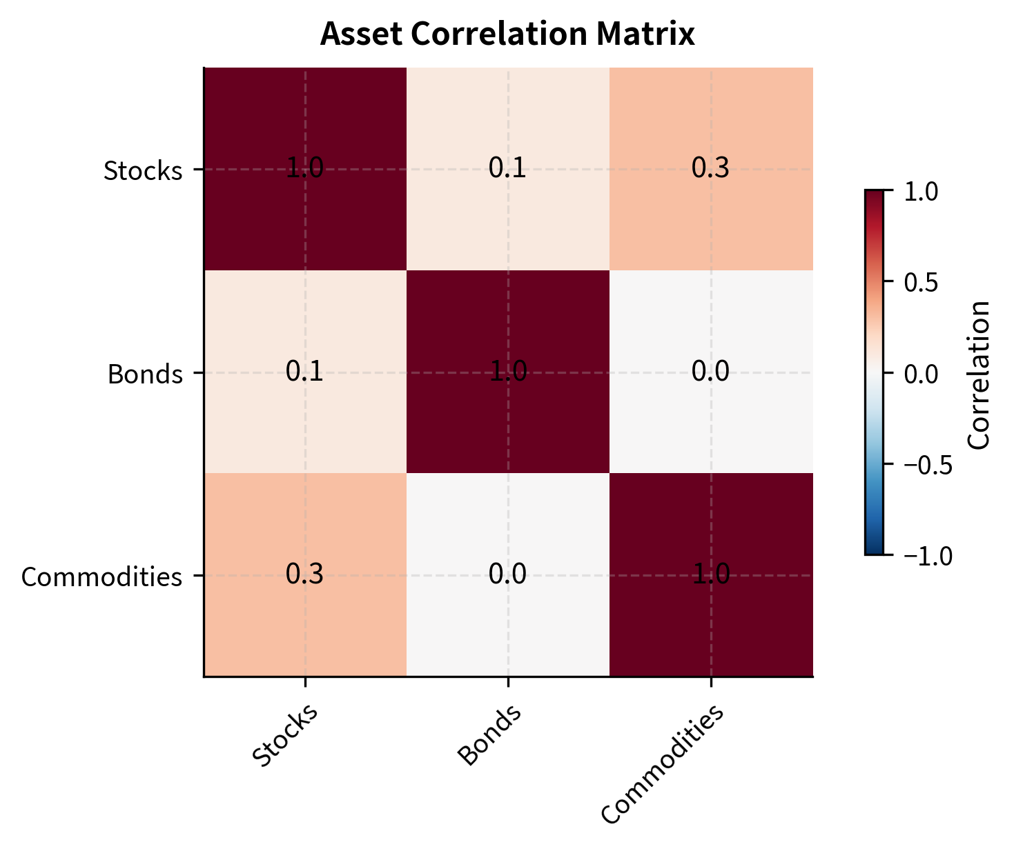
Let's construct an efficient frontier for a portfolio of stocks, bonds, and commodities. This example illustrates how different asset classes with distinct risk-return profiles and correlations combine to form a diversified investment opportunity set:
The covariance matrix confirms the relationships between our assets: stocks and commodities have higher volatility and a moderate positive correlation (0.3), while bonds offer stability with low volatility and low correlation to the other assets. The near-zero correlations between bonds and the other asset classes suggest that bonds will play a crucial role in diversifying portfolio risk.
Now let's compute and visualize the efficient frontier:
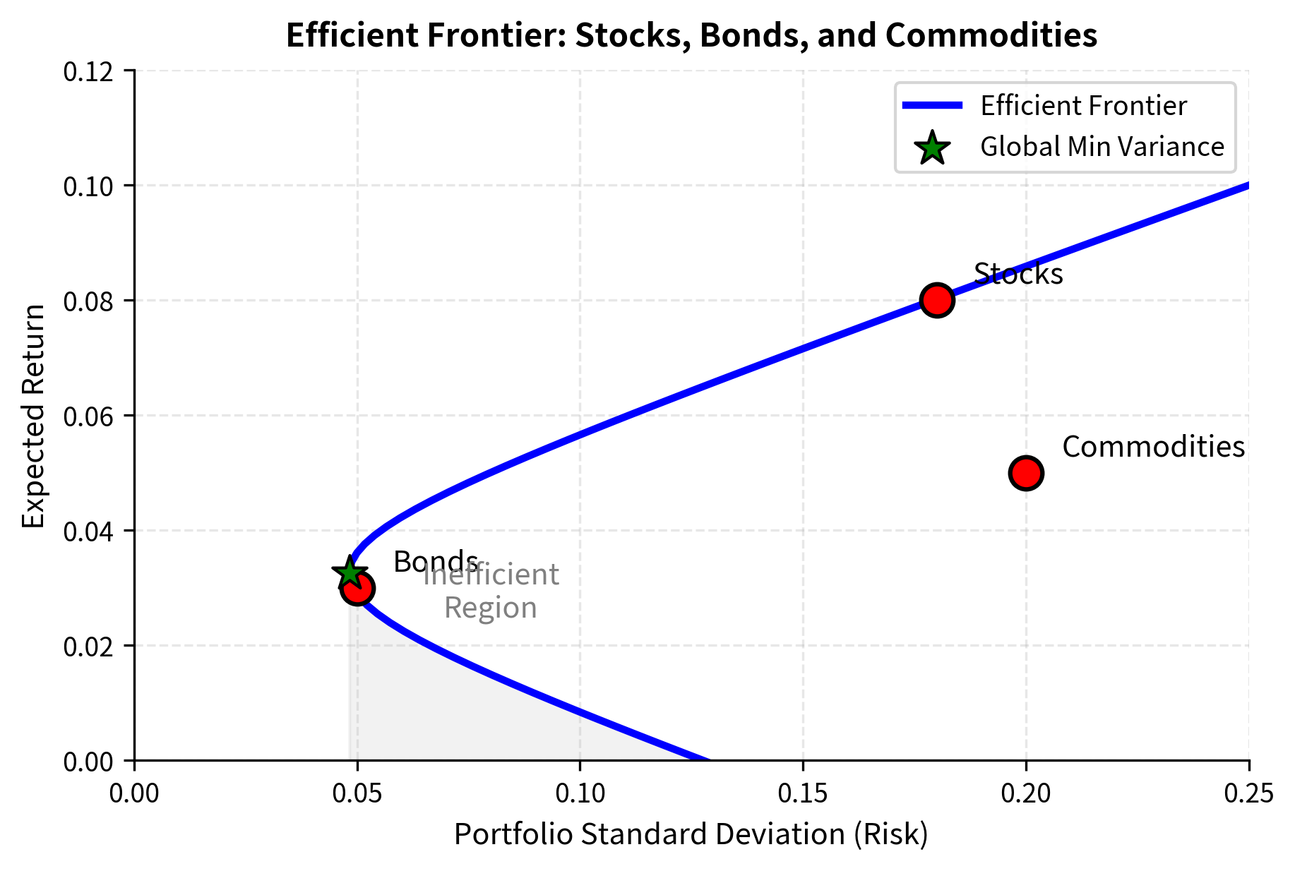
The efficient frontier curve illustrates the optimal risk-return combinations available to investors. The individual assets (red dots) lie inside the frontier, confirming that portfolios combining imperfectly correlated assets offer superior efficiency compared to holding single securities. Notice how the frontier bows outward to the left, demonstrating that diversification creates portfolios with better risk-return characteristics than any individual asset.
The GMV portfolio is heavily weighted toward bonds because of their low volatility. Notice that the GMV portfolio achieves lower risk than any individual asset, demonstrating the power of diversification. Even the lowest-risk asset (bonds at 5% volatility) has higher risk than the optimally diversified GMV portfolio.
Portfolio Composition Along the Frontier
Understanding how portfolio weights change along the efficient frontier provides insight into the risk-return tradeoff. As you move up the frontier seeking higher returns, you must accept more risk, and the portfolio composition shifts accordingly:
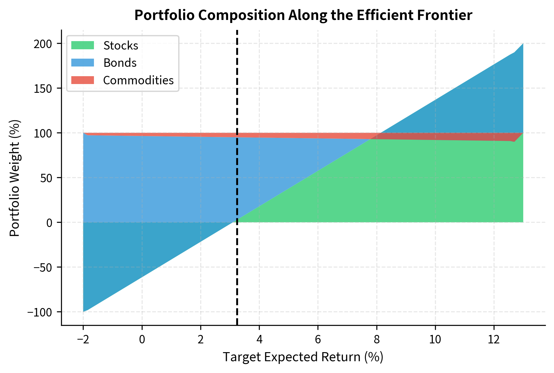
At low target returns (near the GMV portfolio), the allocation is dominated by bonds. As we move up the frontier toward higher returns, the portfolio shifts toward stocks, with commodities providing additional diversification benefits due to their low correlation with bonds. The smooth transition in weights illustrates how the efficient allocation changes continuously as your return target increases.
Quadratic Programming for Portfolio Optimization
For practical applications with many assets and constraints, we use quadratic programming (QP). Quadratic programming is a mathematical optimization technique designed specifically for problems where the objective function is quadratic (involving squared terms) and the constraints are linear. Mean-variance optimization fits this structure perfectly because portfolio variance is a quadratic function of the weights.
The standard QP form is:
where:
- : vector of decision variables
- : symmetric matrix (quadratic term)
- : vector (linear term)
- : matrix and vector defining equality constraints
- : matrix and vector defining inequality constraints
Mean-variance optimization maps directly to this form with and (or for the utility maximization variant). The equality constraints enforce the budget constraint and target return, while inequality constraints can encode position limits, sector constraints, and other practical requirements.
Adding Practical Constraints
Real portfolio optimization often includes additional constraints that reflect regulatory requirements, risk management policies, or investment mandates:
- No short selling: for all . This constraint prevents the portfolio from taking negative positions, which an investor cannot or chooses not to take.
- Maximum position size: (e.g., 10% per asset). This ensures diversification by preventing excessive concentration in any single security.
- Sector constraints: Total exposure to a sector some limit. This prevents the portfolio from becoming overly exposed to a single industry or market segment.
- Turnover constraints: Changes from current portfolio are limited. This controls transaction costs and tax consequences by restricting how much trading occurs.
Let's implement a more realistic optimizer using the cvxpy library:
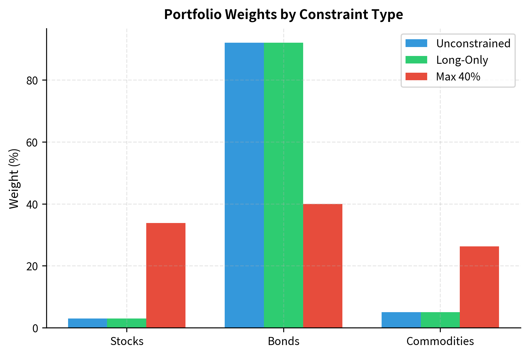
The constrained portfolios have slightly higher risk than the unconstrained GMV portfolio. This is a general result: adding constraints can never improve the optimal objective value. Constraints restrict the feasible region, preventing the optimizer from reaching solutions that might otherwise be optimal. The cost of these constraints appears as slightly higher portfolio risk, but this cost may be acceptable given the practical benefits of avoiding short positions or maintaining diversification.
The Mathematics of Diversification
Diversification is the only "free lunch" in finance. To understand why, let's decompose portfolio variance more carefully. The key insight is that not all risk is equal: some risk affects all assets together (systematic risk), while other risk is unique to individual securities (idiosyncratic risk). Diversification can eliminate the latter but not the former.
Variance Decomposition
Consider an equally-weighted portfolio of assets with identical variance and pairwise correlation . While this is a simplification, it reveals the essential mechanics of diversification. The portfolio variance is:
where:
- : variance of the portfolio
- : number of assets
- : covariance between asset and asset
For the diagonal terms ():
For the off-diagonal terms ():
There are diagonal terms and off-diagonal terms. The diagonal terms represent each asset's own variance contribution, while the off-diagonal terms capture the covariance contributions from all pairs of different assets:
where:
- : variance of each individual asset
- : pairwise correlation between all assets
- : number of assets in the portfolio
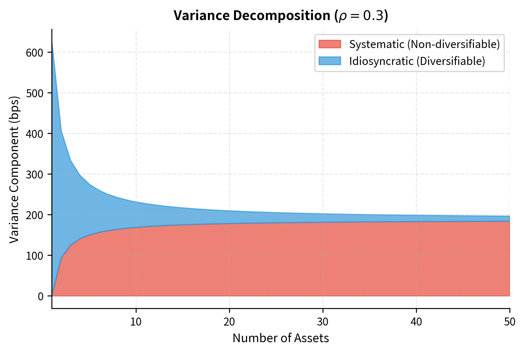
This decomposition separates portfolio variance into two distinct components. The first term, , represents idiosyncratic risk. It depends on the number of assets and shrinks as increases. This is the diversifiable component of risk. The second term, , represents systematic risk. It depends on the correlation between assets and persists regardless of how many assets we hold.
As :
where:
- : limiting portfolio variance
- : pairwise correlation between assets
- : variance of individual assets
This reveals a fundamental insight: diversification can eliminate idiosyncratic risk (the term that vanishes with ), but cannot eliminate systematic risk (the term that persists). No matter how many assets we add to our portfolio, we cannot diversify away the risk that comes from common factors affecting all assets simultaneously. When markets crash, all stocks tend to fall together; this correlated movement represents systematic risk that no amount of stock picking can eliminate.
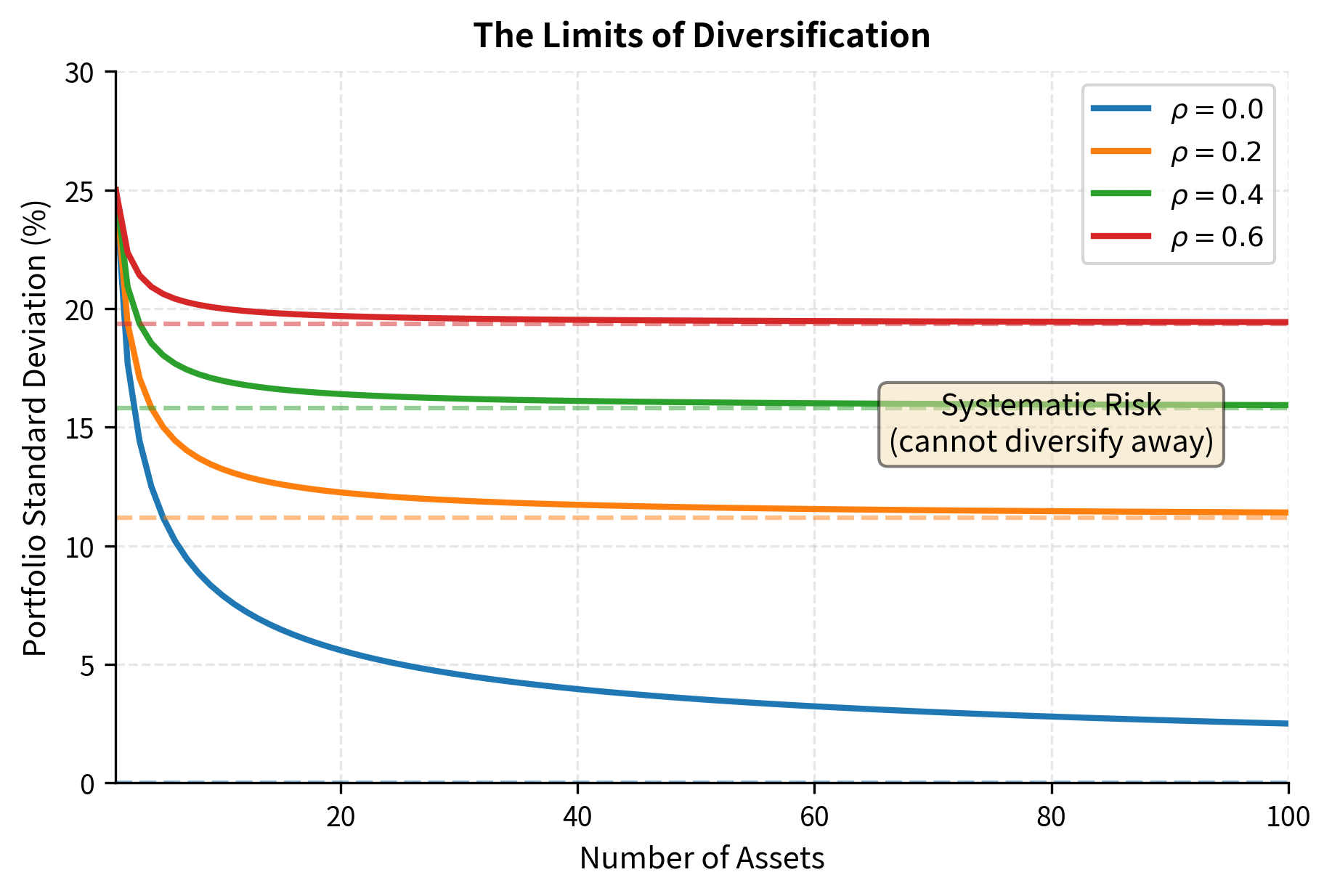
Systematic risk (also called market risk or undiversifiable risk) affects all assets and cannot be eliminated through diversification. Idiosyncratic risk (also called specific or diversifiable risk) is unique to individual assets and approaches zero as portfolio size increases. We'll explore this distinction further in the next chapter on the Capital Asset Pricing Model.
How Many Assets Are Enough?
The figure shows that most diversification benefits are captured with 20-30 assets, depending on correlation. Beyond that, adding assets provides diminishing marginal benefit. This explains why well-diversified portfolios don't need hundreds of positions. The mathematics tells us that each additional asset beyond a certain point contributes very little to further risk reduction, while potentially adding complexity and transaction costs.
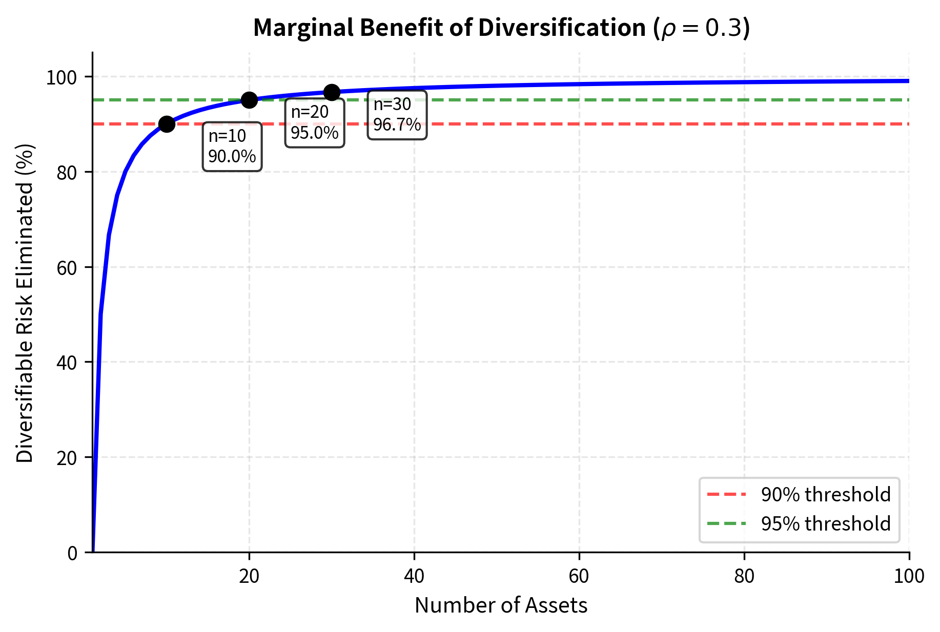
The table results demonstrate that the majority of diversification benefits are realized early. With just 20 assets, nearly 95% of the diversifiable risk is eliminated, confirming that a portfolio does not need hundreds of positions to be well-diversified. This finding has practical implications for portfolio construction: beyond a certain point, adding more securities increases complexity and costs without meaningfully improving the risk-return profile.
Practical Implementation with Real Data
Let's apply mean-variance optimization to a realistic multi-asset portfolio using historical return data:
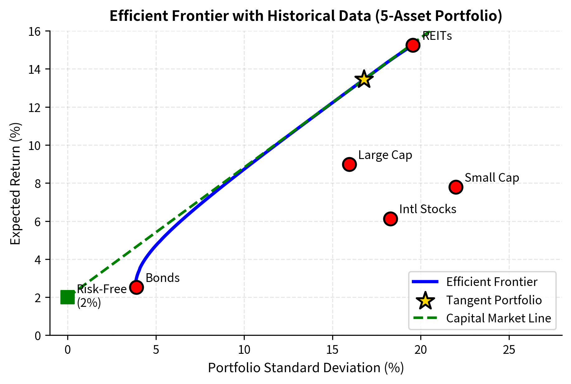
The chart displays the efficient frontier derived from historical data. The Capital Market Line (green dashed) connects the risk-free rate to the tangent portfolio, illustrating the optimal opportunity set available by combining the risk-free asset with the maximal Sharpe ratio portfolio.
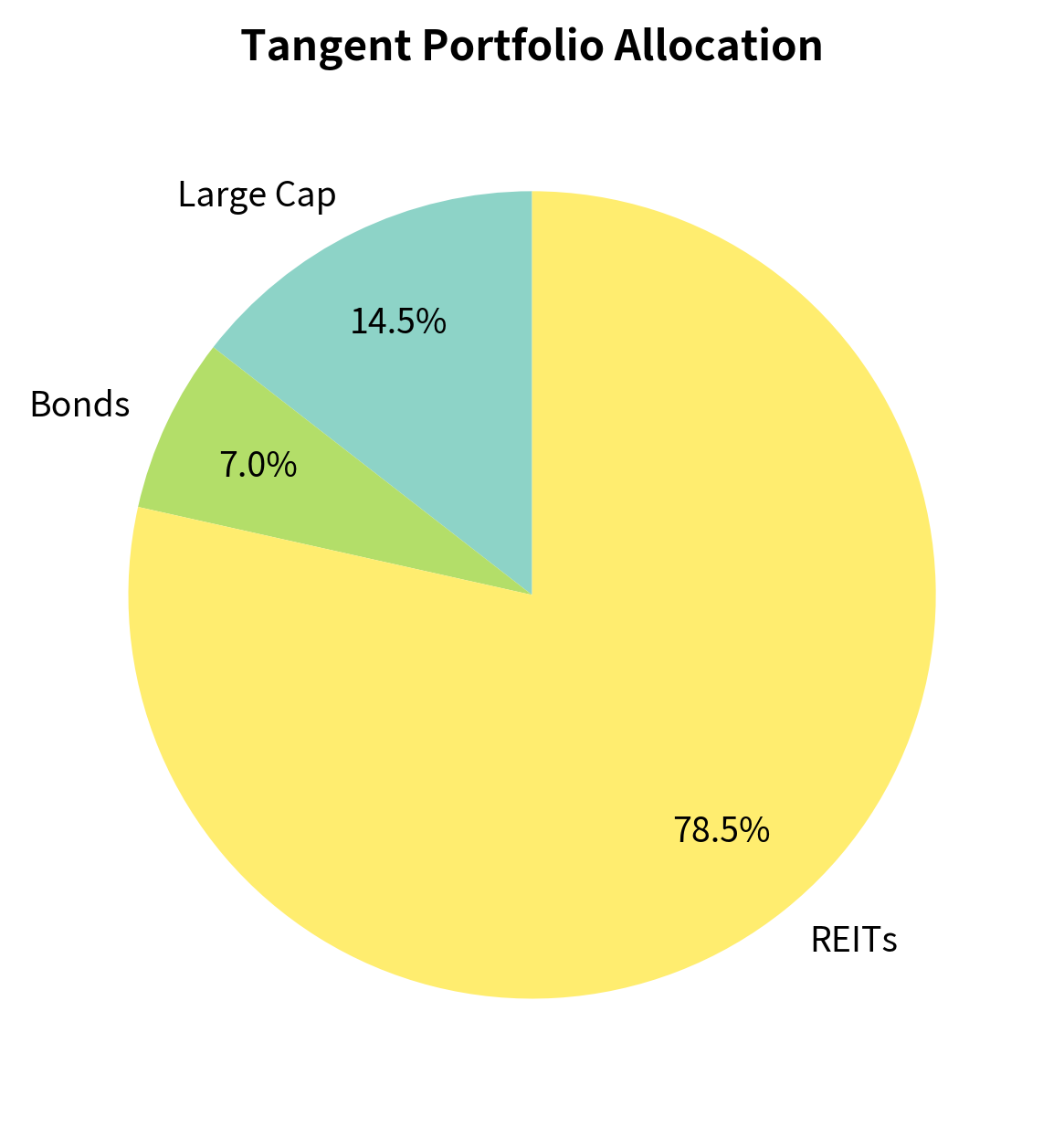
The tangent portfolio maximizes the Sharpe ratio, representing the optimal combination of risky assets. You should hold this portfolio combined with lending or borrowing at the risk-free rate, regardless of your risk preference. This insight leads directly to the Capital Asset Pricing Model, which we'll develop in the next chapter.
Limitations of Mean-Variance Optimization
While mean-variance optimization provides a rigorous framework for portfolio construction, several practical challenges limit its direct application.
Estimation Error
The most significant limitation is sensitivity to input estimation errors. Small changes in expected returns, volatilities, or correlations can lead to dramatically different optimal portfolios. Since we must estimate these parameters from historical data, the resulting portfolios can be highly unstable.
Research has shown that mean-variance optimizers are "error maximizers": they tend to overweight assets with overestimated returns and underweight those with underestimated returns. The expected return estimates are particularly problematic because they have much higher estimation error than covariance estimates.
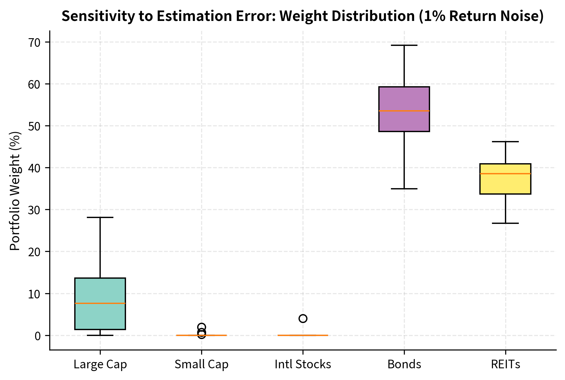
The box plots reveal significant dispersion in the optimal weights for each asset across the simulations. These wide ranges indicate that optimal portfolios are highly sensitive to even small perturbations in expected return inputs, a phenomenon often described as "error maximization."
The weight variability is substantial. A 1% estimation error in expected returns causes some weights to fluctuate by 10 percentage points or more. This instability makes raw mean-variance optimization impractical without additional regularization techniques.
Solutions to Estimation Error
Several approaches address the estimation error problem:
- Shrinkage estimators: Combine sample estimates with prior beliefs (e.g., shrink toward equal weights or a market-cap weighted portfolio)
- Robust optimization: Explicitly account for parameter uncertainty in the optimization
- Resampling methods: Generate multiple parameter sets, optimize each, and average the results
- Constraints: Position limits and other constraints implicitly regularize the optimization
- Black-Litterman model: Combine market equilibrium returns with your views
We'll explore advanced portfolio construction techniques that address these issues in Part IV's later chapters.
Assumptions and Limitations
Beyond estimation error, the mean-variance framework rests on several assumptions worth examining:
-
Quadratic utility or normal returns: Mean-variance is optimal only if returns are normally distributed or you have a quadratic utility function. As we discussed in Part III's chapter on stylized facts, return distributions exhibit fat tails and skewness that violate normality.
-
Single-period framework: The basic model ignores multi-period considerations like rebalancing costs, tax consequences, and changing investment horizons.
-
No transaction costs: Real portfolios face trading costs that mean-variance ignores.
-
Unlimited leverage and short selling: Many investors face constraints that prevent them from implementing the theoretically optimal portfolio.
Despite these limitations, mean-variance optimization remains the foundational framework for portfolio construction. Its insights about diversification, the risk-return tradeoff, and the efficient frontier guide both academic research and practical investment management.
Key Parameters
The key parameters for Mean-Variance Optimization are:
- (Expected Returns): The vector of forecasted returns for each asset. Estimation errors here have the largest impact on portfolio weight stability.
- (Covariance Matrix): Captures the risk of individual assets (diagonal elements) and their co-movements (off-diagonal elements). Positive correlations reduce diversification benefits.
- (Risk-Free Rate): The return on a risk-free asset, used to calculate Sharpe ratios and the Capital Market Line.
- (Risk Aversion): Determines the trade-off between risk and return in the utility maximization formulation ().
- (Weights): The decision variables representing the fraction of capital allocated to each asset. Constraints typically require and (for long-only portfolios).
Summary
This chapter developed the mathematical framework of Modern Portfolio Theory, which transformed investment management from an art to a science.
The key concepts we covered include:
-
Portfolio return and risk: Portfolio expected return is the weighted average of asset returns (), while portfolio variance depends on the full covariance structure ().
-
The efficient frontier: The set of portfolios offering maximum expected return for each level of risk. You should hold a portfolio on this frontier if you are a rational mean-variance investor.
-
Global minimum variance portfolio: The portfolio with the lowest possible variance, given by .
-
Two-fund separation: Any efficient portfolio can be expressed as a combination of two distinct efficient portfolios, simplifying your investment decision.
-
Diversification benefits and limits: Combining assets with less-than-perfect correlation reduces portfolio risk. However, systematic risk (captured by the average correlation) cannot be diversified away, no matter how many assets are included.
-
Practical optimization: Quadratic programming enables efficient frontier computation with realistic constraints on short selling, position sizes, and sector exposures.
-
Estimation error: Mean-variance optimization is highly sensitive to input estimation errors, particularly in expected returns. This sensitivity motivates the regularization techniques and robust methods covered in later chapters.
The framework developed here provides the foundation for the Capital Asset Pricing Model in the next chapter, where we'll see how equilibrium considerations determine the pricing of risk in the market portfolio.
Quiz
Ready to test your understanding? Take this quick quiz to reinforce what you've learned about Modern Portfolio Theory and mean-variance optimization.

Comments