

Learn model calibration techniques for quantitative finance. Master SABR, Heston, GARCH, and Vasicek parameter estimation with practical Python examples.
Choose your expertise level to adjust how many terms are explained. Beginners see more tooltips, experts see fewer to maintain reading flow. Hover over underlined terms for instant definitions.
Calibration and Parameter Estimation in Models
Financial models are only as useful as their connection to reality. A beautifully derived option pricing formula or an elegant interest rate model remains purely theoretical until its parameters are set to match observed market behavior. This process of fitting model parameters to market data is called calibration, and it represents one of the most practically important steps in quantitative finance.
Throughout this book, we've developed sophisticated pricing models: the Black-Scholes framework for options, short-rate models like Vasicek and Hull-White for interest rate derivatives, and GARCH models for volatility dynamics. Each of these models contains parameters that must be determined from data. The volatility parameter in Black-Scholes, the mean reversion speed in the Vasicek model, and the persistence coefficient in GARCH: none of these are given to us by theory. They must be estimated or calibrated.
The distinction between estimation and calibration is subtle but important. Statistical estimation typically uses historical data to find parameters that best explain past observations, often through maximum likelihood or method of moments. Calibration, by contrast, fits parameters so that model outputs match current market prices. It is inherently forward-looking, reflecting the market's consensus view embedded in traded prices. In practice, quantitative finance uses both approaches, often in combination.
This chapter develops the theory and practice of calibration. We'll formalize the calibration problem, explore different objective functions and optimization techniques, and work through practical examples. Crucially, we'll also address the dangers of overfitting: the tendency to fit noise rather than signal when models have too many free parameters relative to the information content of the data.
The Calibration Problem
Calibration begins with a model that produces prices or other observable quantities as a function of parameters. To understand this formally, let denote model prices for a vector of parameters . The market provides observed prices for instruments. The calibration problem seeks parameters such that model prices are as close as possible to market prices .
The process of determining model parameters by minimizing the discrepancy between model-implied prices and observed market prices. A well-calibrated model reproduces current market quotes while remaining stable and economically sensible.
This simple description masks several important choices. What does "as close as possible" mean? How do we measure discrepancy? How do we search for optimal parameters? And what happens when perfect agreement is impossible because the model cannot reproduce all market prices simultaneously? These questions form the core of calibration theory and drive the methodological choices we explore throughout this chapter.
Why Models Can't Fit Perfectly
Consider calibrating the Black-Scholes model to a set of option prices. Black-Scholes assumes constant volatility for all options on the same underlying. But as we discussed in the chapter on implied volatility and the volatility smile, the market assigns different implied volatilities to options with different strikes and maturities. No single value of can reproduce all observed option prices.
This fundamental tension arises because models simplify reality. The Black-Scholes model ignores jumps, stochastic volatility, and many other market features. When we calibrate, we're finding the best compromise: the parameter values that make the model least wrong across the calibration instruments. This perspective is essential for understanding calibration not as a search for "truth" but as a practical optimization that acknowledges model limitations.
More sophisticated models reduce but never eliminate this tension. The Heston stochastic volatility model has five parameters and can capture some smile dynamics, but it still cannot perfectly match every market price. Adding parameters improves fit but introduces new problems: more complex optimization landscapes, greater risk of overfitting, and parameters that may be poorly identified. The art of calibration lies in finding the right balance between model flexibility and parsimony.
Mathematical Formulation
Let denote the model price for instrument given parameters . The calibration problem is typically formulated as an optimization problem. We seek parameters that minimize some measure of discrepancy between what the model predicts and what the market shows us. Mathematically, this takes the form:
where:
- : the optimal set of parameters that we seek
- : a vector of model parameters over which we optimize
- : a loss function measuring the discrepancy between model and market prices
- : the set of feasible parameters, typically constrained by economic requirements such as positivity of volatility or valid correlation bounds
This formulation captures the essence of calibration: we have a loss function that quantifies how poorly the model matches the market, and we search over the space of allowable parameters to find those that minimize this loss. The choice of loss function profoundly affects the calibration outcome, as different functions emphasize different aspects of fit quality.
The most common loss functions include several variations that each serve distinct purposes:
Sum of squared errors (SSE):
where:
- : number of calibration instruments
- : model price for instrument given parameters
- : observed market price for instrument
This is the simplest and most intuitive loss function. It sums the squared differences between model and market prices across all instruments. Squaring ensures that positive and negative errors don't cancel, and larger errors receive disproportionately more penalty than smaller ones. This makes SSE particularly sensitive to outliers, which can be either an advantage (outliers might indicate important mispricings) or a disadvantage (outliers might represent data errors).
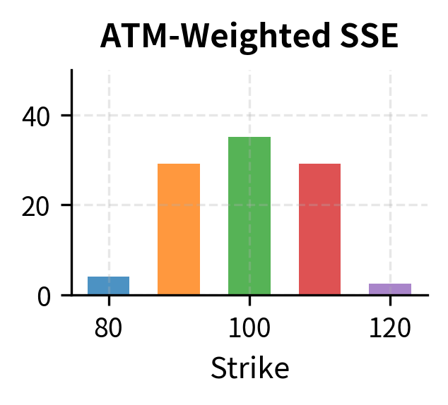
Weighted sum of squared errors:
where:
- : weight assigned to instrument
- : number of calibration instruments
- : model price for instrument given parameters
- : observed market price for instrument
Weighted SSE introduces flexibility by allowing different instruments to contribute differently to the objective. You might assign higher weights to more liquid instruments whose prices are more reliable, or to instruments that are most relevant to your trading book. The weights encode your beliefs about which prices are most important to match accurately.
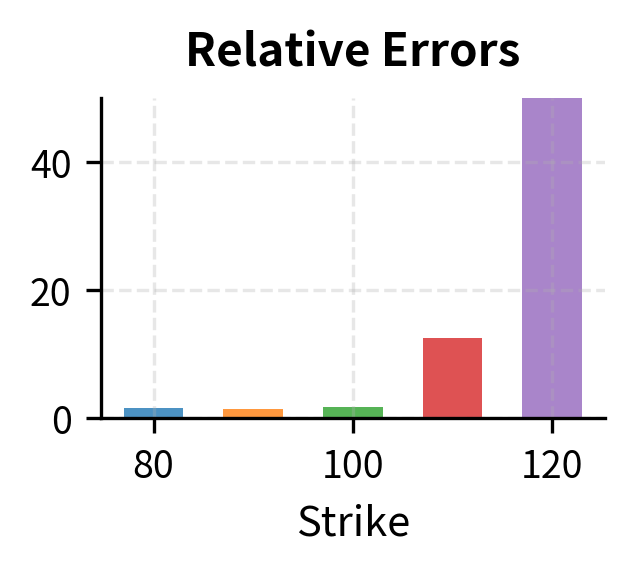
Relative errors:
where:
- : number of calibration instruments
- : model price for instrument
- : observed market price for instrument
Relative errors normalize by price, so a $1 error on a $100 instrument counts the same as a $0.10 error on a $10 instrument. This prevents expensive instruments from dominating the calibration simply because their absolute price differences are larger. Relative errors are particularly useful when calibrating across instruments with widely varying price levels.
The choice of loss function matters significantly. Weighting allows you to emphasize certain instruments, perhaps at-the-money options where liquidity is highest, or specific maturities relevant to your trading book. Relative errors prevent large-priced instruments from dominating the calibration. Understanding these trade-offs is essential for designing calibration procedures that produce parameters suited to your specific use case.
Objective Functions for Calibration
The loss function defines what "good calibration" means. Different objectives lead to different calibrated parameters, and the choice should reflect how the model will be used. A model calibrated for pricing exotic derivatives may need different parameter values than one calibrated for risk management, even if based on the same underlying framework.
Price-Based Calibration
The most direct approach minimizes differences between model and market prices. This makes sense when the model will be used for pricing similar instruments. If you're calibrating to vanilla option prices and will use the model to price exotic options, matching vanilla prices closely ensures consistency between the pricing of hedging instruments and the exotic.
For options, a common choice is to calibrate in volatility space rather than price space. Instead of minimizing price errors, we minimize implied volatility errors:
where:
- : implied volatility derived from the model price for instrument
- : observed market implied volatility for instrument
- : weight for instrument
- : number of calibration instruments
This approach has several advantages. First, implied volatilities are more comparable across strikes and maturities than raw prices. A one-volatility-point error means roughly the same thing whether the option is at-the-money or far out-of-the-money, whereas price errors can vary dramatically depending on the option's delta. Second, the objective function surface tends to be better behaved numerically, with smoother gradients that make optimization more reliable. Third, you typically think in volatility terms, so errors expressed in volatility points are more interpretable.
Bid-Ask Spread Considerations
Market prices are not single values; they come with bid-ask spreads that reflect the cost of transacting and the uncertainty about fair value. A sophisticated calibration might seek parameters such that model prices fall within observed bid-ask bounds rather than matching midpoint prices exactly:
where:
- : market bid price, the highest price at which someone is willing to buy
- : market ask price, the lowest price at which someone is willing to sell
- : model price
- : loss function to minimize
- : model parameters
This formulation acknowledges that any price within the spread is consistent with the market. When perfect fit is impossible, the model at least shouldn't produce prices outside observed trading bounds. This is particularly relevant for less liquid instruments where bid-ask spreads are wide and the "true" price is genuinely uncertain.
Maximum Likelihood Estimation
For time-series models like GARCH or short-rate models estimated from historical data, maximum likelihood estimation (MLE) provides a principled framework rooted in statistical theory. Given observations and a model specifying the conditional density , the log-likelihood is:
where:
- : log-likelihood function, measuring how probable the observed data is under the model
- : vector of model parameters
- : number of time series observations
- : conditional probability density specified by the model
- : observation at time
The intuition behind MLE is elegant: we seek parameters that make the observed data as probable as possible under the model. If the model with certain parameters would rarely generate data like what we observed, those parameters are unlikely to be correct. Conversely, parameters that would frequently generate data similar to our observations are good candidates for the true values.
Maximizing yields parameters that make the observed data most probable under the model. As we discussed in the chapter on modeling volatility and GARCH, this is the standard approach for fitting GARCH models to return data.
MLE has attractive statistical properties: under regularity conditions, the estimator is consistent (converges to true parameters as sample size grows), asymptotically efficient (achieves the lowest possible variance among consistent estimators), and asymptotically normal (enabling confidence interval construction). These theoretical guarantees make MLE the gold standard for parameter estimation when a likelihood function is available.
Combined Objectives
In practice, calibration often combines multiple objectives to satisfy different requirements simultaneously. A short-rate model might be calibrated to match the current yield curve exactly while also fitting to cap and swaption prices as closely as possible. This requires a hierarchical approach or a composite objective with appropriate weights.
Optimization Techniques
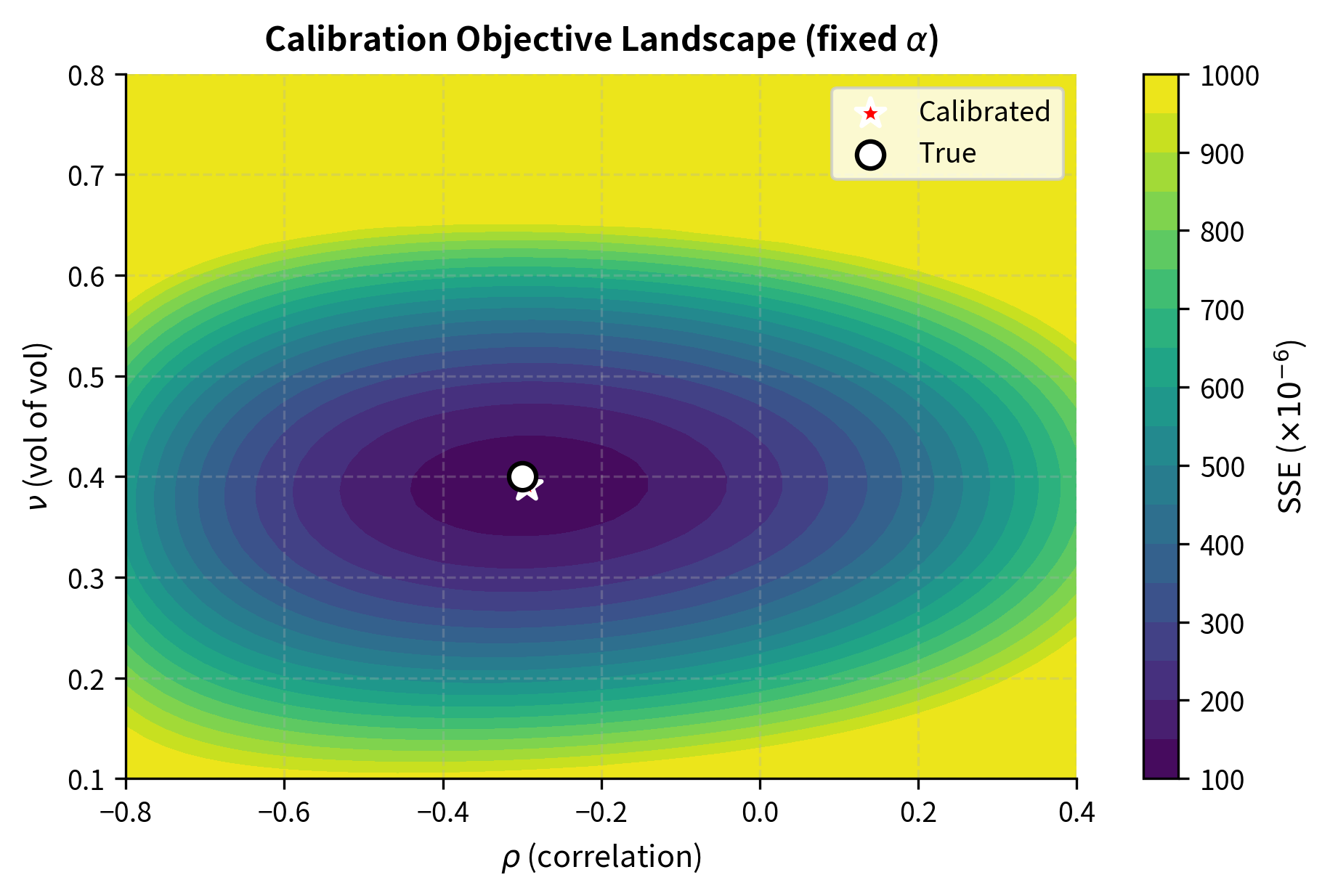
Once we've specified an objective function, we need algorithms to find the minimizing parameters. Calibration optimization presents particular challenges: objective functions may be non-convex with multiple local minima, parameter spaces may be constrained, and model evaluations (especially for derivatives requiring Monte Carlo or PDE methods) may be computationally expensive. Understanding the landscape of available optimization techniques is essential for practical calibration.
Gradient-Based Methods
When the objective function is smooth and its gradient is available (analytically or via automatic differentiation), gradient-based methods are efficient. The simplest is gradient descent, which follows the direction of steepest descent to iteratively reduce the objective:
where:
- : parameter vector at iteration
- : step size (learning rate) controlling how far we move at each iteration
- : gradient of the objective function, pointing in the direction of steepest increase
This update rule iteratively moves parameters in the direction of steepest descent (opposite the gradient) to reduce the loss function value. The gradient tells us which direction leads uphill; by moving in the opposite direction, we descend toward lower values of the loss function.
More sophisticated variants like BFGS and L-BFGS use quasi-Newton updates to approximate the Hessian matrix, achieving faster convergence near optima. These methods build up information about the curvature of the objective function, allowing them to take more intelligent steps that account for how the gradient itself changes.
Gradient methods find local minima efficiently but may get stuck in suboptimal solutions if the objective is non-convex. Good initialization is critical; starting near the global minimum dramatically increases the chance of finding it. This limitation motivates the global optimization methods discussed next.
Global Optimization
For complex models with non-convex objectives, global optimization methods explore the parameter space more thoroughly by maintaining diversity in their search:
Differential evolution maintains a population of candidate solutions that evolve through mutation, crossover, and selection. It's derivative-free and handles constraints naturally, making it popular for financial calibration. The algorithm mimics biological evolution: candidate parameter vectors compete based on their fitness (objective function value), with successful vectors influencing future generations.
Simulated annealing allows uphill moves with decreasing probability, escaping local minima early in the search while converging to a local minimum as the "temperature" cools. This metaphor comes from metallurgy, where controlled cooling produces stronger materials by allowing atoms to settle into low-energy configurations.
Basin hopping combines local optimization with random restarts, finding multiple local minima and selecting the best. This pragmatic approach acknowledges that a single local search may not find the global minimum and systematically explores multiple starting points.
These methods are more robust to initialization but computationally more expensive. A common hybrid strategy uses global optimization to find a promising region, then refines with a gradient-based method. This combines the exploration capability of global methods with the efficiency of local methods.
Constraints and Regularization
Model parameters often have economic constraints that must be respected. Volatility must be positive. Mean-reversion speeds should be positive for stability. Correlation parameters must lie in . These constraints can be enforced through several mechanisms:
Constrained optimization: Algorithms like SLSQP or trust-region methods handle bounds and general constraints directly, ensuring that every parameter vector evaluated during optimization satisfies the constraints.
Parameter transformation: Reparameterizing to ensure constraints are automatically satisfied is an elegant alternative. For a parameter , optimize over instead; then any value of maps to a valid positive . For a correlation , use for unconstrained . This transformation approach converts a constrained problem into an unconstrained one.
Penalty methods: Add a large penalty to the objective when constraints are violated:
where:
- : penalized objective function that combines fit quality and constraint satisfaction
- : original loss function measuring fit to data
- : penalty parameter controlling the severity of constraint violation penalties
- : inequality constraints (positive values indicate violation)
- : model parameters
When is large, any constraint violation adds a substantial penalty, steering the optimization toward feasible solutions.
Regularization adds penalties for large parameter values or parameter instability, encouraging parsimonious solutions:
where:
- : regularized objective function balancing fit and parameter magnitude
- : original loss function
- : regularization strength controlling the trade-off
- : squared Euclidean norm of the parameters
This L2 regularization (ridge penalty) shrinks parameters toward zero, reducing overfitting when many parameters compete to explain limited data. By penalizing large parameter values, regularization expresses a preference for simpler explanations and reduces the model's sensitivity to noise.
Calibrating Implied Volatility Surfaces
Let's work through a practical example: calibrating a parametric implied volatility surface to market option quotes. This is a common first step in derivatives pricing: obtaining a smooth volatility surface from noisy market quotes that can be used for pricing and hedging.
We'll use the SABR model, a popular stochastic volatility model with a closed-form approximation for implied volatility. The SABR model has become an industry standard for interest rate options and is widely used for equity options as well. It specifies the forward price dynamics through two coupled stochastic differential equations:
where:
- : forward price at time
- : stochastic volatility at time
- : initial volatility ( in some notations), setting the overall level of the volatility smile
- : volatility of volatility (vol-vol), determining how much the volatility itself fluctuates
- : elasticity parameter, controlling the relationship between the forward price and local volatility
- : standard Brownian motions with correlation
- : correlation coefficient between the forward price and volatility processes
The first equation describes the forward price evolution with a Constant Elasticity of Variance (CEV) backbone determined by . When , the forward follows log-normal dynamics, while gives normal dynamics. The second equation drives the stochastic volatility process with vol-of-vol , allowing volatility itself to evolve randomly over time.
The correlation parameter is particularly important because it determines whether large price moves tend to coincide with high or low volatility. Negative correlation (common in equity markets) means that downward price moves are associated with volatility increases, generating the characteristic negative skew observed in equity option markets.
Hagan et al. derived an approximate formula for implied volatility as a function of strike and forward . This approximation is remarkably accurate for typical market conditions and enables rapid calibration without numerically solving the underlying stochastic differential equations:
where:
- : current forward price
- : strike price
- : time to expiration
- : initial volatility level
- : elasticity parameter
- : correlation between Brownian motions
- : volatility of volatility
- : moneyness normalized by volatility, measuring how far the strike is from at-the-money in volatility-adjusted terms
- : skew adjustment function that modifies implied volatility based on the correlation structure
The formula decomposes into three interpretable parts. The first fraction establishes the primary volatility level, scaled appropriately for the moneyness. The skew adjustment term modifies this level based on how correlation between price and volatility affects options at different strikes. The final bracket in the formula provides a time-dependent correction factor that accounts for how the smile dynamics evolve as we look further into the future.
This formula looks intimidating, but it's straightforward to implement. Let's calibrate SABR to synthetic option data.
Now let's generate synthetic market data from known SABR parameters and add noise:
The noisy market data represents what we'd observe from real quotes, where bid-ask spreads, stale prices, and measurement errors introduce random deviations from any theoretical model. Now let's calibrate SABR to recover the parameters:
The calibration successfully recovers parameters close to the true values, despite the noise in the data. The small RMSE in basis points indicates that the model provides an excellent fit to market observations. Let's visualize the calibrated smile against the market data:
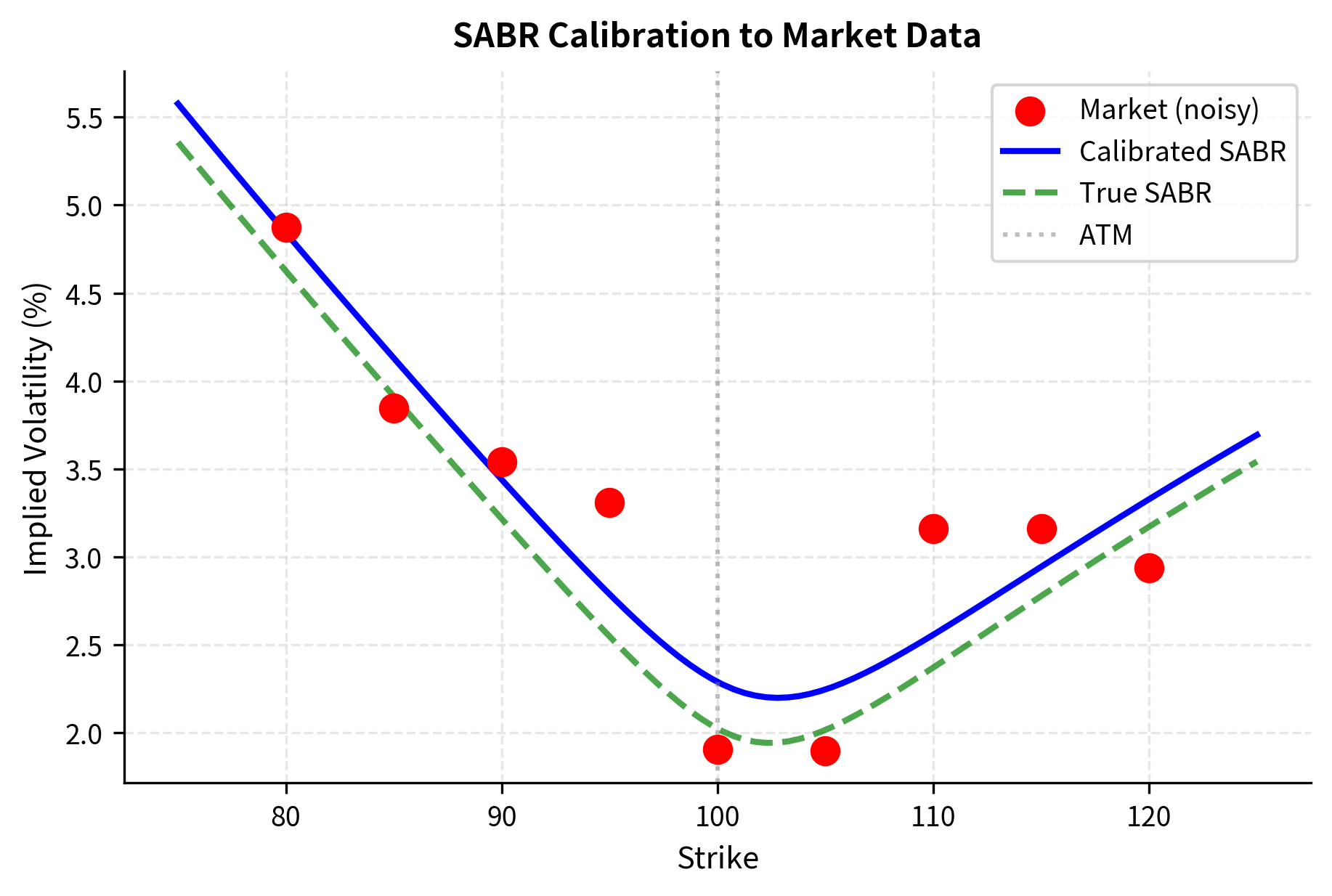
The calibrated curve smoothly interpolates through the noisy market quotes, providing a volatility surface suitable for pricing options at any strike.
Key Parameters
The key parameters for the SABR model are:
- : Initial volatility level. Controls the overall height of the implied volatility ATM.
- : Elasticity parameter. Determines the relationship between asset price and volatility (backbone). Often fixed (e.g., to 0.5) during calibration.
- : Correlation between the asset price and volatility. Controls the skew (slope) of the volatility smile.
- : Volatility of volatility (vol-vol). Controls the curvature (convexity) of the volatility smile.
Calibrating Short-Rate Models to the Yield Curve
Short-rate models, as we covered in the chapter on short-rate interest rate models, specify the dynamics of the instantaneous interest rate. For pricing, these models must first be calibrated to match current market yields. Let's calibrate the Vasicek model to a given yield curve.
The Vasicek model is one of the foundational short-rate models, valued for its analytical tractability and intuitive interpretation. It specifies the evolution of the instantaneous short rate through the following stochastic differential equation:
where:
- : instantaneous short rate at time
- : mean reversion speed, determining how quickly the rate returns to equilibrium
- : long-term mean rate, the equilibrium level toward which rates are pulled
- : volatility of the rate, controlling the magnitude of random fluctuations
- : standard Brownian motion driving the random component
The drift term ensures mean reversion: when , the drift is negative, pulling the rate down, and when , the drift is positive, pushing it up. This mean-reverting behavior is economically sensible, as interest rates tend to fluctuate around some equilibrium level rather than wandering arbitrarily far. The strength of this pull is governed by : larger values mean faster reversion to the mean.
Under the Vasicek model, zero-coupon bond prices have a closed-form solution. This analytical tractability is one of the model's key advantages, enabling rapid calibration and pricing:
where:
- : price at time of a bond maturing at
- : instantaneous short rate at time
- : current time
- : maturity time
- : Vasicek model parameters
- : duration-like factor that captures how bond prices respond to rate changes
- : convexity adjustment that accounts for the nonlinear relationship between rates and bond prices
The function resembles modified duration in some ways, measuring the sensitivity of the bond price to changes in the short rate. The function incorporates convexity effects and the impact of the long-term mean on bond pricing.
The continuously compounded yield can be derived from the bond price formula:
where:
- : continuously compounded yield for maturity
- : zero-coupon bond price
- : Vasicek bond price coefficients defined above
- : instantaneous short rate
- : current time
- : maturity time
This relationship shows how the model's parameters translate into observable yields, which is precisely what we need for calibration.
Let's create a synthetic market yield curve and calibrate the Vasicek model to it:
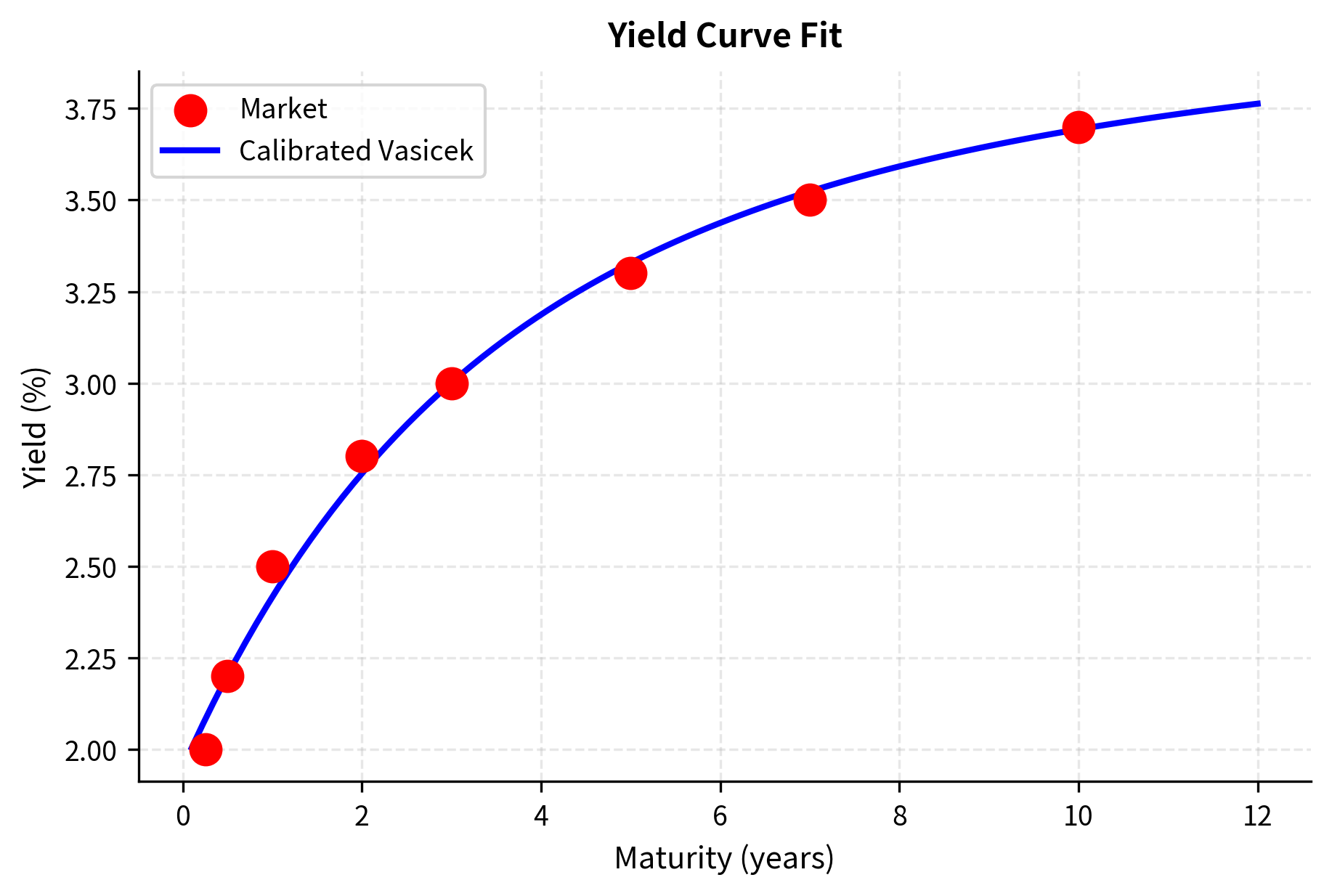
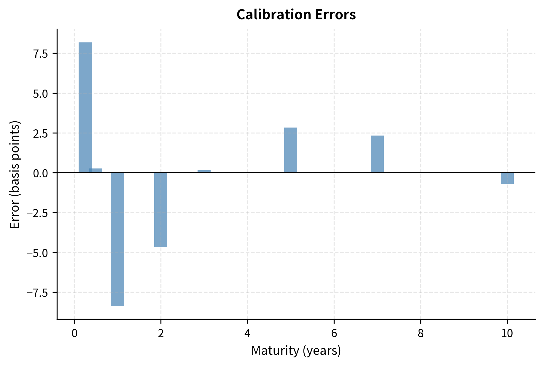
The calibrated parameters () are economically realistic. The Vasicek model fits the yield curve reasonably well, but note the small systematic errors. This illustrates a key limitation: the Vasicek model has only four parameters, and typical yield curves have more degrees of freedom. More flexible models like Hull-White can achieve exact calibration by allowing time-varying parameters, as we discussed in the chapter on advanced interest rate models.
Key Parameters
The key parameters for the Vasicek model are:
- : Mean reversion speed. Determines how quickly the short rate returns to the long-term mean .
- : Long-term mean rate. The equilibrium level to which the interest rate converges.
- : Volatility of the short rate. Controls the magnitude of random rate fluctuations.
- : Current instantaneous short rate. The starting point for the rate process.
Calibrating the Heston Stochastic Volatility Model
For equity derivatives, the Heston model is the workhorse stochastic volatility model. It captures the essential features of equity markets, including volatility clustering and the leverage effect (the tendency for volatility to increase when prices fall), while remaining analytically tractable. The model specifies joint dynamics for the asset price and its variance:
where:
- : asset price at time
- : instantaneous variance at time (note: variance, not volatility)
- : drift rate of the asset price
- : Brownian motions with correlation
- : initial variance, the starting level for the variance process
- : speed of mean reversion for variance, determining how fast variance returns to its long-run level
- : long-term variance level, the equilibrium to which variance is pulled
- : volatility of variance (vol of vol), controlling how much the variance itself fluctuates
- : correlation between spot price and variance, typically negative for equities
The variance process follows a Cox-Ingersoll-Ross (CIR) process, which prevents negative variance (when the Feller condition is satisfied) and exhibits mean reversion to the long-run level . The square root in the variance diffusion term ensures that variance fluctuations scale appropriately with the variance level: when variance is high, it can fluctuate more; when variance is low, fluctuations are dampened.
The correlation parameter is crucial for capturing the leverage effect. In equity markets, is typically negative, meaning that downward price moves tend to coincide with increases in variance. This generates the characteristic negative skew observed in equity option markets, where out-of-the-money puts are more expensive than equally out-of-the-money calls.
The Heston model has a semi-closed-form solution for European option prices via characteristic functions. The call price is:
where:
- : call option price
- : asset price at time
- : strike price
- : risk-free interest rate
- : time to expiration
- : probabilities derived from the characteristic function, representing the delta and the risk-neutral exercise probability respectively
The probabilities and are computed by numerical integration of the characteristic function. While this requires numerical methods, it is vastly more efficient than Monte Carlo simulation and enables rapid calibration.
Let's implement calibration to option prices:
Now let's generate market data and calibrate:
The Heston calibration recovers parameters close to the true values, though note the small discrepancies. This is typical; market option prices don't perfectly follow the Heston model, so calibration finds the best compromise. Additionally, the output confirms the Feller condition is satisfied (), ensuring the variance process remains strictly positive.
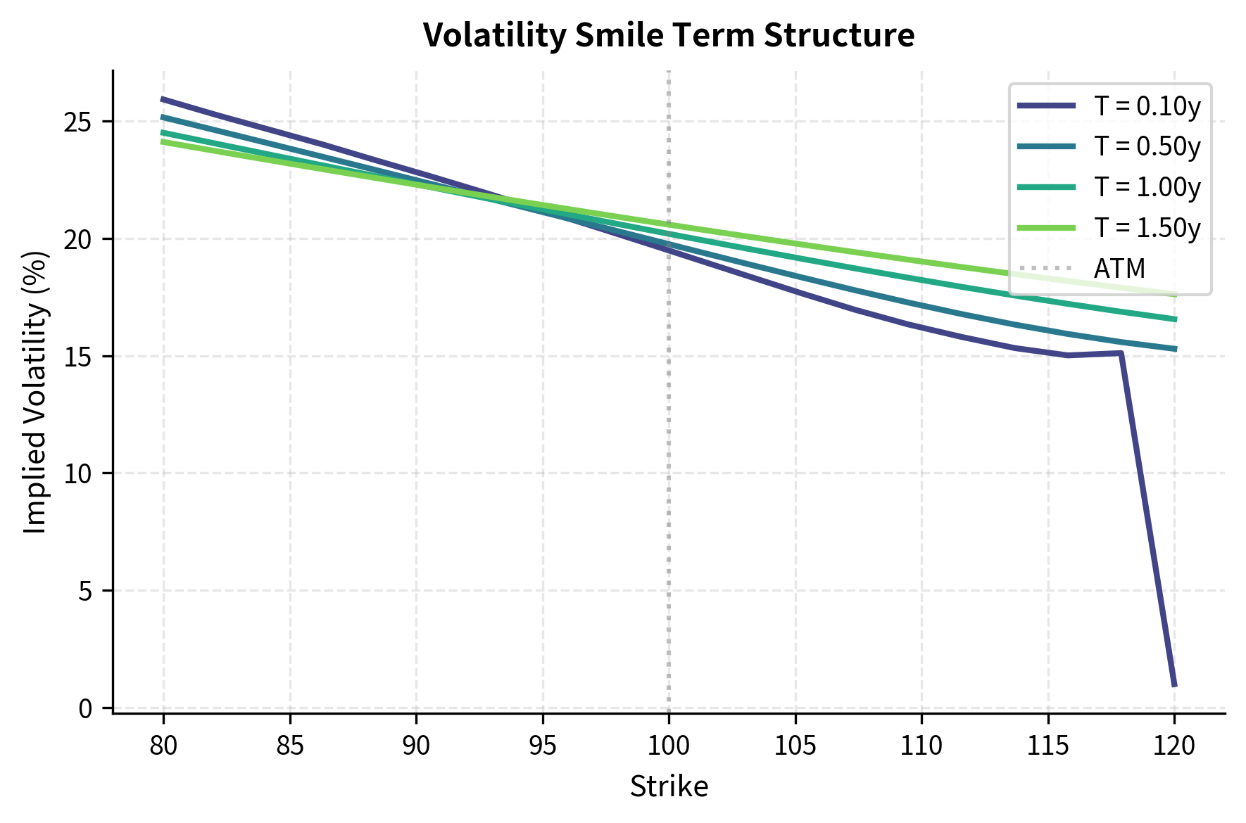
To visualize the model's behavior, we compute the implied volatility surface corresponding to the calibrated parameters. This involves generating Heston prices across a grid of strikes and maturities, then inverting the Black-Scholes formula to find the implied volatility for each.
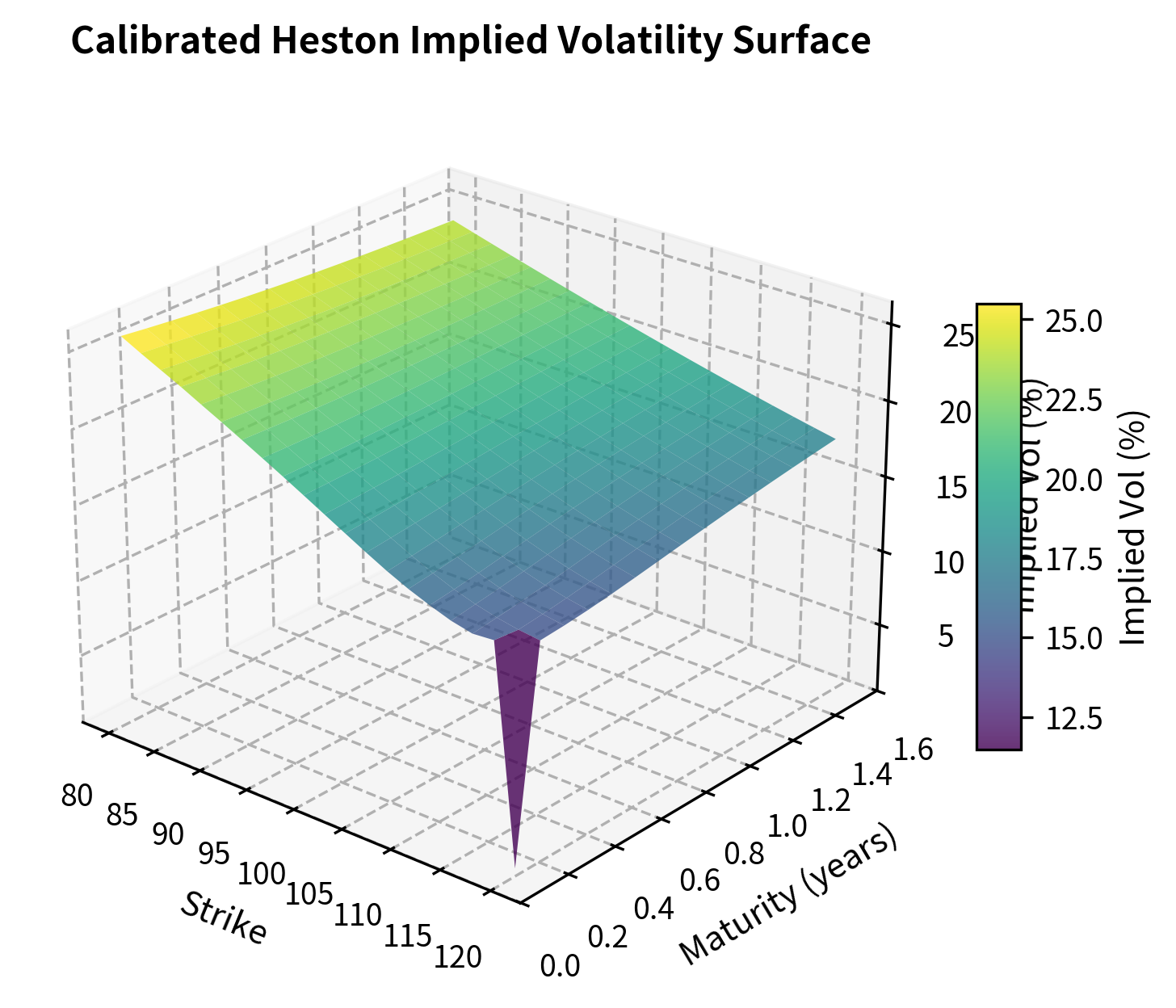
The calibrated surface shows the characteristic negative skew (higher implied volatility for low strikes) produced by negative correlation , and the term structure effects from mean reversion and vol of vol parameters.
Key Parameters
The key parameters for the Heston model are:
- : Initial variance. The starting level of the variance process.
- : Mean reversion speed of variance. Determines how fast variance returns to .
- : Long-run average variance. The level to which variance converges over time.
- : Volatility of variance (vol-of-vol). Controls the variance of the variance process itself, affecting the smile curvature and kurtosis.
- : Correlation between the asset price and variance processes. Controls the skew of the implied volatility surface.
Maximum Likelihood Estimation for Time-Series Models
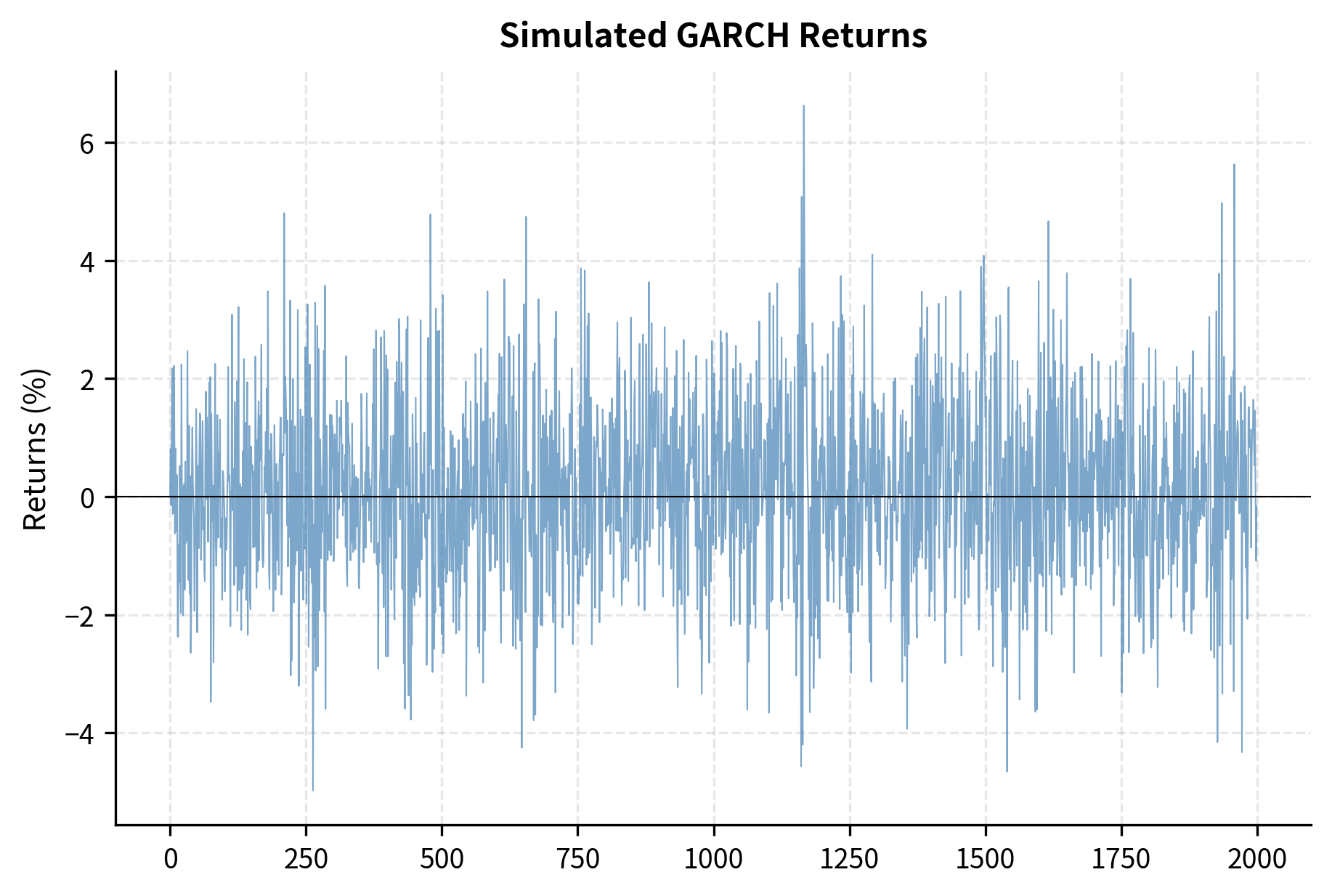
While calibration to market prices is essential for pricing derivatives, statistical estimation from historical data remains important for risk modeling and forecasting. Let's demonstrate MLE for the GARCH(1,1) model, building on our discussion in the chapter on modeling volatility.
The GARCH(1,1) model has become the standard framework for modeling time-varying volatility in financial returns. It captures volatility clustering, the empirical observation that large returns tend to be followed by large returns, and small returns tend to be followed by small returns. The model specifies:
where:
- : return at time
- : mean return
- : return innovation (residual), the unexpected component of the return
- : conditional variance, the variance of returns conditional on past information
- : standard normal random variable driving the innovation
- : GARCH parameters controlling the variance dynamics
The conditional variance depends on three components. The baseline variance provides a floor that prevents variance from collapsing to zero. The recent market shock (the ARCH term) allows large return surprises to increase future variance immediately. The previous period's variance (the GARCH term) captures the persistence of volatility over time. Together, these components enable the model to capture volatility clustering, where high-volatility periods tend to persist.
The persistence of volatility is measured by the sum . When this sum is close to 1 (but less than 1 for stationarity), shocks to volatility decay slowly, consistent with the long memory observed in financial return volatility.
The log-likelihood for observations is derived from the assumption that innovations are conditionally normal:
where:
- : log-likelihood function, measuring how probable the observed returns are under the model
- : number of observations
- : conditional variance at time , computed recursively from the GARCH equation
- : residual at time , equal to
- : mathematical constant pi
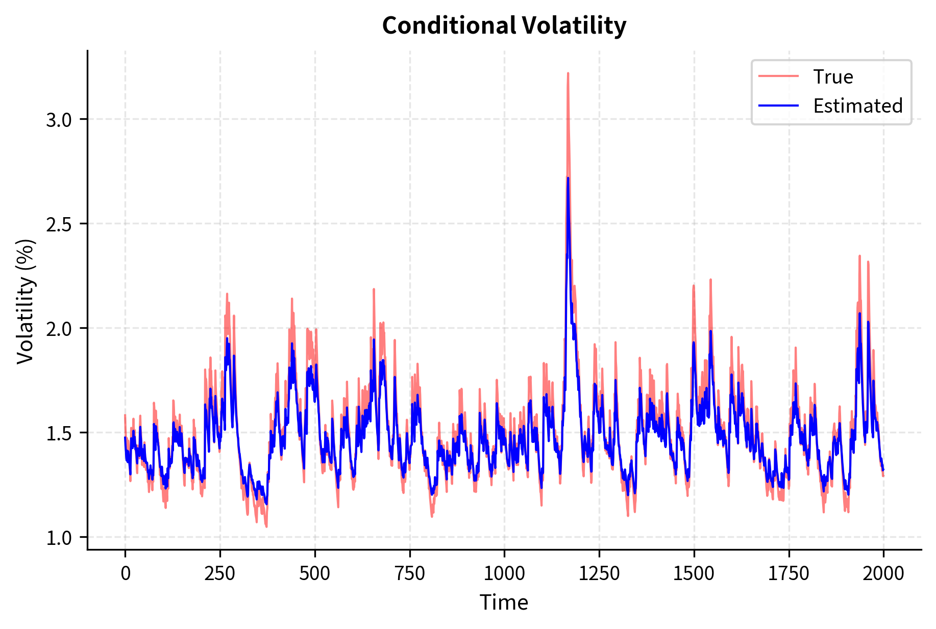
The likelihood penalizes two things: large variances (through the term) and large standardized residuals (through the term). Good parameters balance these competing objectives by having variances that are neither too large nor too small, accurately tracking the true volatility of returns.
MLE recovers the GARCH parameters accurately. The persistence measure close to 1 indicates that volatility shocks decay slowly, consistent with the stylized facts of financial returns we discussed earlier in this part.
Key Parameters
The key parameters for the GARCH(1,1) model are:
- : Constant baseline variance term.
- : ARCH parameter. Measures the reaction of volatility to recent return shocks (innovations).
- : GARCH parameter. Measures the persistence of past variance.
- : Mean return parameter.
Overfitting and Model Selection
A critical danger in calibration is overfitting: fitting the noise in calibration data rather than the underlying signal. An overfit model matches calibration instruments perfectly but generalizes poorly to new data or instruments not in the calibration set. Understanding and preventing overfitting is essential for building models that work in practice.
The tendency of flexible models to fit noise in calibration data, leading to unstable parameters and poor out-of-sample performance. Overfit models appear excellent on calibration instruments but fail on new data.
Symptoms of Overfitting
Overfitting manifests in several characteristic ways that you learn to recognize:
-
Parameter instability is a key warning sign: if calibrating to slightly different data (different days, or excluding some instruments) produces dramatically different parameters, the model is likely overfit. Well-identified parameters should be robust to small data changes. When parameters jump around erratically, the model is fitting noise rather than signal.
-
Extreme parameter values suggest the model is stretching to fit noise. A calibrated vol of vol near the boundary of the feasible region, or mean reversion speeds approaching infinity, indicate that the optimization is exploiting flexibility rather than capturing genuine dynamics. Economic intuition often provides bounds on reasonable parameter values; violating these bounds is a warning sign.
-
Poor out-of-sample performance is the definitive test. If a model fits calibration instruments with high precision but badly misprices similar instruments not in the calibration set, it has overfit. This is why you always reserve some data for testing.
Sources of Overfitting
The primary sources of overfitting include:
-
Too many parameters relative to data. A model with free parameters fitted to data points risks overfitting when is large relative to . This becomes acute when instruments are highly correlated (e.g., options at adjacent strikes) so that effective degrees of freedom are fewer than the raw count suggests. Ten options at closely spaced strikes provide less information than ten options at widely spaced strikes.
-
Noisy data. Market prices contain measurement error, stale quotes, and temporary dislocations. Flexible models can fit these artifacts, which don't persist. The model learns the specific noise pattern in today's data rather than the underlying structure.
-
Model misspecification. This creates a subtle form of overfitting: when the true data-generating process differs from the model, extra parameters may compensate for model inadequacy rather than capturing real effects. The model may achieve good in-sample fit by distorting its parameters to approximate dynamics it fundamentally cannot represent.
Preventing Overfitting
Several strategies mitigate overfitting:
Regularization adds penalties for complex solutions:
where:
- : penalty function (e.g., parameter magnitude or parameter variability)
- : regularization parameter controlling the trade-off between fit and complexity
By adding a cost for large or complex parameter configurations, regularization encourages the optimization to find simpler solutions that generalize better.
Cross-validation holds out some data for testing. Fit parameters using a subset of instruments, then evaluate fit quality on held-out instruments. This directly measures generalization by testing on data not used during calibration.
Information criteria like AIC and BIC provide principled model selection that balances fit quality against model complexity:
where:
- : Akaike Information Criterion
- : Bayesian Information Criterion
- : number of parameters
- : sample size
- : maximized likelihood value
Both penalize additional parameters; BIC penalizes more heavily for large samples. Lower values indicate better models when balancing fit and complexity.
Parameter bounds derived from economic intuition prevent extreme values. If historical estimates suggest mean reversion speeds between 0.5 and 3, constraining calibration to this range prevents overfitting to noise.
Let's demonstrate cross-validation for model selection:
The cross-validation RMSE estimates the expected prediction error on unseen data. A low value indicates the model generalizes well and is not simply fitting the noise in the specific calibration set.
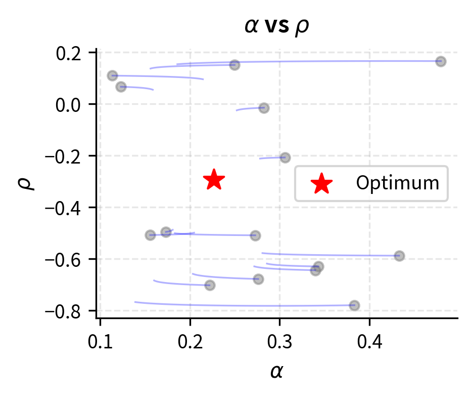
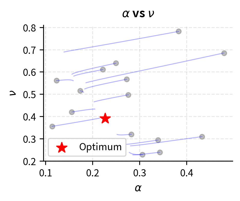
Parameter Stability Analysis
Examining how calibrated parameters change with different data provides insight into identification and overfitting:
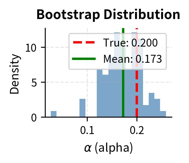
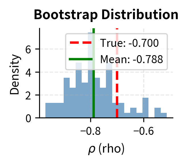
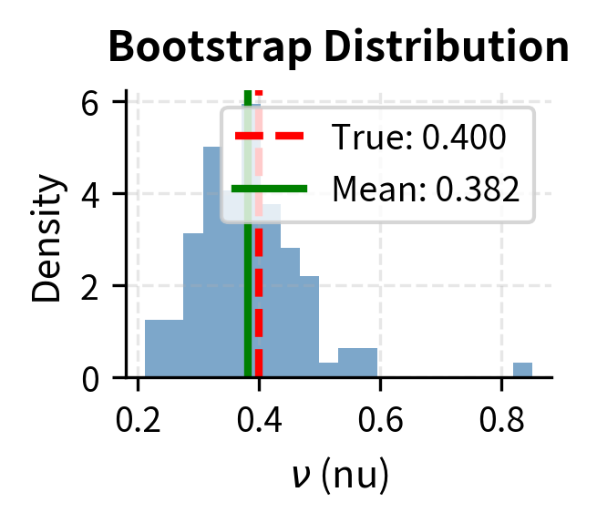
The bootstrap analysis reveals parameter uncertainty. Low coefficient of variation (CV) indicates stable, well-identified parameters. High CV suggests the parameter is poorly determined and may be subject to overfitting.
Practical Calibration Workflows
Real-world calibration involves systematic workflows that address data quality, optimization robustness, and ongoing monitoring.
Data Preparation
Before calibration, market data must be cleaned and prepared:
-
Quote filtering removes stale, erroneous, or illiquid quotes. Options with very low open interest or wide bid-ask spreads may contain noise that degrades calibration.
-
Consistency checks ensure data is arbitrage-free. Calendar spreads (options at different maturities) and butterfly spreads should have non-negative value. Violations suggest data errors.
-
Standardization converts raw prices to a common format. Options at different maturities should use appropriate day-count conventions and settlement rules.
Multi-Start Optimization
Non-convex objectives require multiple optimization runs from different starting points:
The multi-start calibration confirms the stability of our solution, converging to the same parameters as the initial run. This suggests the optimization has likely found the global minimum.
Calibration Monitoring
Production calibration systems monitor for problems:
-
Fit quality metrics track calibration RMSE over time. Sudden increases may indicate market regime changes or data problems.
-
Parameter drift monitors how calibrated parameters evolve. Large daily changes suggest instability or overfitting.
-
Constraint binding checks whether parameters hit bounds frequently. Consistently binding constraints suggest the feasible region may need adjustment or the model is inadequate.
Limitations and Impact
Calibration is both essential and inherently limited. Understanding these limitations is crucial for using calibrated models appropriately.
The fundamental limitation is that calibration fits a model to a snapshot of market prices, but markets evolve continuously. A model calibrated this morning may be miscalibrated by afternoon if volatility spikes or correlations shift. This creates a tension between calibration frequency (recalibrating often to stay current) and stability (frequent recalibration produces noisy parameters that complicate hedging).
Another deep limitation stems from model choice. Calibration finds the best parameters for a given model, but cannot tell you whether the model itself is appropriate. A poorly specified model, no matter how carefully calibrated, will misprice instruments that depend on dynamics it doesn't capture. The residual errors after calibration provide some signal: systematic patterns in residuals suggest model inadequacy, but distinguishing model error from noise remains challenging.
The impact of calibration extends throughout derivatives pricing and risk management. Well-calibrated models enable consistent pricing between standard instruments (used for hedging) and exotics (being priced). They support model-based hedging strategies, where Greeks computed from calibrated models guide position adjustments. And they provide the foundation for risk measurement, where consistent valuation across a portfolio requires coherent model parameters.
Looking ahead, the parameters we calibrate here will be essential inputs for portfolio optimization in Part IV, where we'll construct optimal portfolios using expected returns and covariances estimated from data. Similarly, in Part V on risk management, calibrated volatility models and correlation structures underpin Value-at-Risk and stress testing calculations. The techniques developed here, including optimization, cross-validation, and stability analysis, are foundational skills that appear throughout quantitative finance.
Summary
This chapter developed the theory and practice of model calibration, one of the most practically important skills in quantitative finance.
We established the calibration problem: finding model parameters that minimize the discrepancy between model outputs and market observations. Different objective functions (such as price errors, implied volatility errors, or likelihood functions) encode different notions of fit quality. The choice should reflect the model's intended use.
Optimization techniques range from gradient-based methods for smooth, well-behaved objectives to global optimization for complex, non-convex landscapes. Practical calibration uses multi-start optimization, appropriate constraints, and regularization to find robust solutions.
Through worked examples, we calibrated the SABR model to option implied volatilities, the Vasicek model to yield curves, and the Heston model to option prices across strikes and maturities. Each example illustrated the workflow: define the objective, choose an optimizer, verify results, and assess fit quality.
The dangers of overfitting received substantial attention. Overfit models match calibration data well but generalize poorly. Warning signs include parameter instability, extreme values, and poor out-of-sample performance. Mitigation strategies include regularization, cross-validation, information criteria for model selection, and bootstrap analysis of parameter uncertainty.
Calibration is not a one-time exercise but an ongoing process. Production systems continuously recalibrate as market data updates, monitor fit quality, and flag potential problems. The goal is not mathematical perfection (which is impossible given model limitations) but practical adequacy: models that price consistently, hedge effectively, and remain stable under normal market conditions.
Quiz
Ready to test your understanding? Take this quick quiz to reinforce what you've learned about calibration and parameter estimation in financial models.

Comments