

Master regression analysis for finance: estimate market beta, test alpha significance, diagnose heteroskedasticity, and apply multi-factor models with robust standard errors.
Regression Analysis for Financial Relationships
Financial markets are built on relationships. The return of a stock depends on broad market movements. Bond yields respond to changes in interest rate expectations. Currency pairs move with economic fundamentals. Understanding these relationships, including quantifying their strength, testing their significance, and using them for prediction, requires a powerful statistical framework: regression analysis.
Regression analysis provides the foundation for many core concepts in quantitative finance. When you hear that a stock has a "beta of 1.2," that number comes from a regression. When you claim to generate "alpha" as a portfolio manager, you're making a statement about regression intercepts. When we test whether momentum or value factors explain returns, we're running regressions. The Capital Asset Pricing Model, which we'll explore in depth in Part IV, is fundamentally a regression model relating expected returns to market exposure.
Building on the statistical inference techniques from Part I and the time-series models from the previous chapters, this chapter develops regression analysis with a focus on financial applications. We'll start with the ordinary least squares framework, then apply it to estimate factor exposures, conduct hypothesis tests, and diagnose the problems that arise when regression meets financial time series data. By the end, you'll be able to estimate a stock's market beta, test whether it generates statistically significant alpha, and correct for the autocorrelation and heteroskedasticity that plague financial data.
The Ordinary Least Squares Framework
Regression analysis models the relationship between a dependent variable and one or more explanatory variables. In finance, we often want to explain asset returns using factor returns, or forecast prices using economic indicators. The power of regression lies in its ability to decompose variation: separating what can be explained by observable factors from what remains unexplained. This decomposition forms the basis for understanding risk, measuring performance, and building predictive models.
The Simple Linear Model
Consider a linear relationship between a dependent variable and an independent variable . The core idea is straightforward: we believe that changes in produce predictable changes in , but this relationship is obscured by random noise. Our goal is to uncover the underlying systematic relationship despite this noise.
where:
- : observation of the dependent variable for observation
- : corresponding independent variable
- : intercept, representing the expected value of when
- : slope coefficient, representing the change in for a one-unit change in
- : error term capturing the variation in not explained by
The intercept anchors the regression line at a specific level. In financial contexts, when we regress stock returns on market returns, the intercept represents the return we would expect when the market return is exactly zero. This parameter captures the baseline performance that exists independently of market movements.
The slope coefficient is the heart of the regression. It tells us the marginal effect: for every one-unit increase in , we expect to change by units on average. In the context of finance, if in a stock-versus-market regression, then a 1% market move corresponds to an expected 1.3% move in the stock. This amplification (or dampening, if ) characterizes the stock's systematic risk profile.
The error term represents everything we cannot observe or measure that affects . This includes firm-specific news, measurement error, and the influence of countless unmeasured factors. We assume it has zero mean, constant variance, and is uncorrelated across observations; these are assumptions we'll scrutinize carefully later. These assumptions matter because they determine whether our statistical inference is valid and whether our confidence intervals are trustworthy.
The OLS Estimator
Having specified the model, we need a method to estimate the unknown parameters and . Ordinary least squares takes an intuitive approach: find the line that minimizes the total squared distance between observed values and the line's predictions. Why squared distances? Squaring serves two purposes: it treats positive and negative deviations symmetrically, and it penalizes large errors more heavily than small ones, making the estimator sensitive to outliers but also more efficient when errors are normally distributed.
Ordinary least squares finds the estimators by minimizing the sum of squared residuals :
where:
- : sum of squared residuals to be minimized
- : dependent and independent variable observations for item
- : intercept and slope coefficients to be estimated
- : number of observations
This objective function creates a surface in two-dimensional parameter space. The optimal parameter values correspond to the lowest point on this surface, where the total squared error reaches its minimum. Finding this minimum requires calculus: we take derivatives with respect to each parameter and set them equal to zero.
Taking partial derivatives with respect to and and setting them to zero yields the normal equations:
The first equation has an intuitive interpretation. It says that the sum of residuals must equal zero, meaning the regression line must pass through the center of mass of the data. Positive errors exactly balance negative errors. From the first equation, dividing by yields , which gives . This result confirms that the fitted line passes through the point , the sample means of both variables.
Substituting this into the second equation eliminates :
Rearranging terms to group and :
Using the algebraic identity to center the variables:
gives:
where:
- : estimated slope coefficient
- : estimated intercept
- : sample means of and
- : sample covariance between the independent and dependent variables
- : sample variance of the independent variable
The slope coefficient equals the covariance between and divided by the variance of . This formula reveals the essential logic of regression. The numerator, covariance, measures how and move together. The denominator, variance, normalizes this co-movement by the spread of . The ratio measures how much moves, on average, when moves by one unit. If has high variance, we have more information to estimate the relationship precisely, so we divide by a larger number. The intercept ensures the regression line passes through the point .
Matrix Formulation
For multiple regression with explanatory variables, the matrix formulation is essential. The scalar derivation becomes unwieldy with multiple variables, but matrix algebra provides an elegant and general solution. This formulation also reveals the geometric interpretation: OLS finds the projection of the dependent variable onto the space spanned by the explanatory variables.
We write:
where:
- : vector of observations
- : matrix of explanatory variables (including a column of ones for the intercept)
- : vector of coefficients
- : vector of errors
The design matrix stacks all observations of all explanatory variables. Each row represents one observation, and each column represents one variable. The first column typically consists of ones, which corresponds to the intercept term. This structure allows us to handle any number of explanatory variables using the same mathematical framework.
As we covered in Part I's treatment of linear algebra, the OLS solution minimizes the objective function . We expand the quadratic form and take the derivative:
The expansion follows from distributing the transpose operation and recognizing that produces a scalar. Since a scalar equals its own transpose, we have , allowing us to combine these terms.
Taking the derivative with respect to :
Setting the derivative to zero yields the normal equations:
These normal equations have a clear interpretation. The term captures the correlation between each explanatory variable and the dependent variable. The term is the Gram matrix of the regressors, encoding their variances and mutual correlations. The normal equations balance these two components.
Assuming is invertible:
where:
- : vector of estimated coefficients
- : design matrix of explanatory variables
- : vector of dependent variable observations
Intuitively, this generalizes the scalar slope formula . The term captures the covariation between regressors and the dependent variable, while normalizes by the variance-covariance structure of the regressors, effectively "dividing" by the variance while adjusting for correlations between explanatory variables. When regressors are correlated with each other, the matrix inverse accounts for this overlap, ensuring that each coefficient represents the unique contribution of its variable after controlling for all others.
This closed-form solution is the foundation for all OLS regression analysis. Its existence guarantees that we can always compute the optimal coefficients directly, without iterative optimization. The requirement that be invertible means no explanatory variable can be a perfect linear combination of others, a condition known as the absence of perfect multicollinearity.
Factor Exposures and the CAPM Beta
The single most important application of regression in finance is estimating how an asset responds to systematic risk factors. This relationship, called factor exposure or factor loading, tells us how much of an asset's return can be explained by common factors versus idiosyncratic risk. Understanding factor exposures is essential for portfolio construction, risk management, and performance evaluation. You cannot diversify away systematic risk, so measuring these exposures is crucial for understanding and pricing that risk.
The Market Model
The simplest factor model relates individual stock returns to market returns. This approach, developed in the early days of modern finance, recognizes that stocks tend to move together because they are all affected by common economic forces. Broad market movements, driven by changes in interest rates, economic growth expectations, and investor sentiment, influence virtually all stocks to varying degrees.
where:
- : return on stock at time
- : return on the market index
- : beta coefficient, measuring sensitivity to market movements
- : alpha coefficient, measuring return unexplained by the market
- : idiosyncratic error term
This is called the market model or single-index model. The coefficient measures the stock's systematic risk, representing how much the stock moves when the market moves. A stock with rises 1.2% on average when the market rises 1%, and falls 1.2% when the market falls 1%. This amplification makes high-beta stocks more volatile than the market and more risky in a portfolio context. Conversely, a stock with is defensive: it dampens market movements rather than amplifying them.
The idiosyncratic error term captures firm-specific events: earnings surprises, management changes, product launches, and other news that affects only this particular company. Unlike systematic risk, idiosyncratic risk can be diversified away by holding many stocks, because positive surprises at some firms offset negative surprises at others.
The beta coefficient measures an asset's sensitivity to market movements. Mathematically, it equals the covariance of the asset's return with the market return, divided by the variance of the market return:
where:
- : beta coefficient for asset
- : covariance between asset and market returns
- : variance of market returns
This formula has a clear interpretation. The numerator measures how the asset and market move together. The denominator normalizes by market volatility. A stock that moves perfectly with the market, with the same magnitude, has beta equal to one. The market portfolio itself always has a beta of exactly one.
Excess Returns and the CAPM
The Capital Asset Pricing Model, which we'll derive formally in Part IV, states that the expected excess return on any asset should be proportional to its beta. This fundamental result connects risk and return: assets with higher systematic risk must offer higher expected returns to compensate investors for bearing that risk. The CAPM provides the theoretical foundation for using beta as a measure of risk.
where:
- : expected excess return on asset
- : expected market risk premium
- : risk-free interest rate
- : asset's beta
The left side represents the expected return above the risk-free rate, which is the premium investors demand for taking risk. The right side says this premium should equal beta times the market risk premium. An asset with beta of 1.5 should earn 1.5 times the market risk premium, because it carries 1.5 times the market's systematic risk.
To test this empirically, we regress excess returns:
where:
- : excess return on asset
- : excess return on the market portfolio
- : Jensen's alpha measuring abnormal performance
- : systematic risk exposure
- : idiosyncratic error term
If the CAPM holds, the intercept should be zero. This is because all expected return should be explained by beta exposure to the market. A significantly positive alpha suggests the stock earns more than its risk-adjusted required return: it generates excess risk-adjusted performance. A negative alpha means the stock underperforms relative to its risk. This interpretation makes alpha regression one of the most scrutinized statistical tests in investment management. Every active manager claims to generate alpha, and every client wants evidence to support that claim.
Implementing Beta Estimation
Let's estimate the market beta for a stock using historical data. We'll use synthetic data that mimics realistic return characteristics.
Now we estimate the regression using both manual calculation and statsmodels:
The manual estimates closely match the true parameters used to generate the data, confirming the accuracy of the OLS formulas.
Let's also use statsmodels for a complete regression output:
The regression output provides the coefficient estimates along with standard errors, t-statistics, and p-values. Let's visualize the relationship:
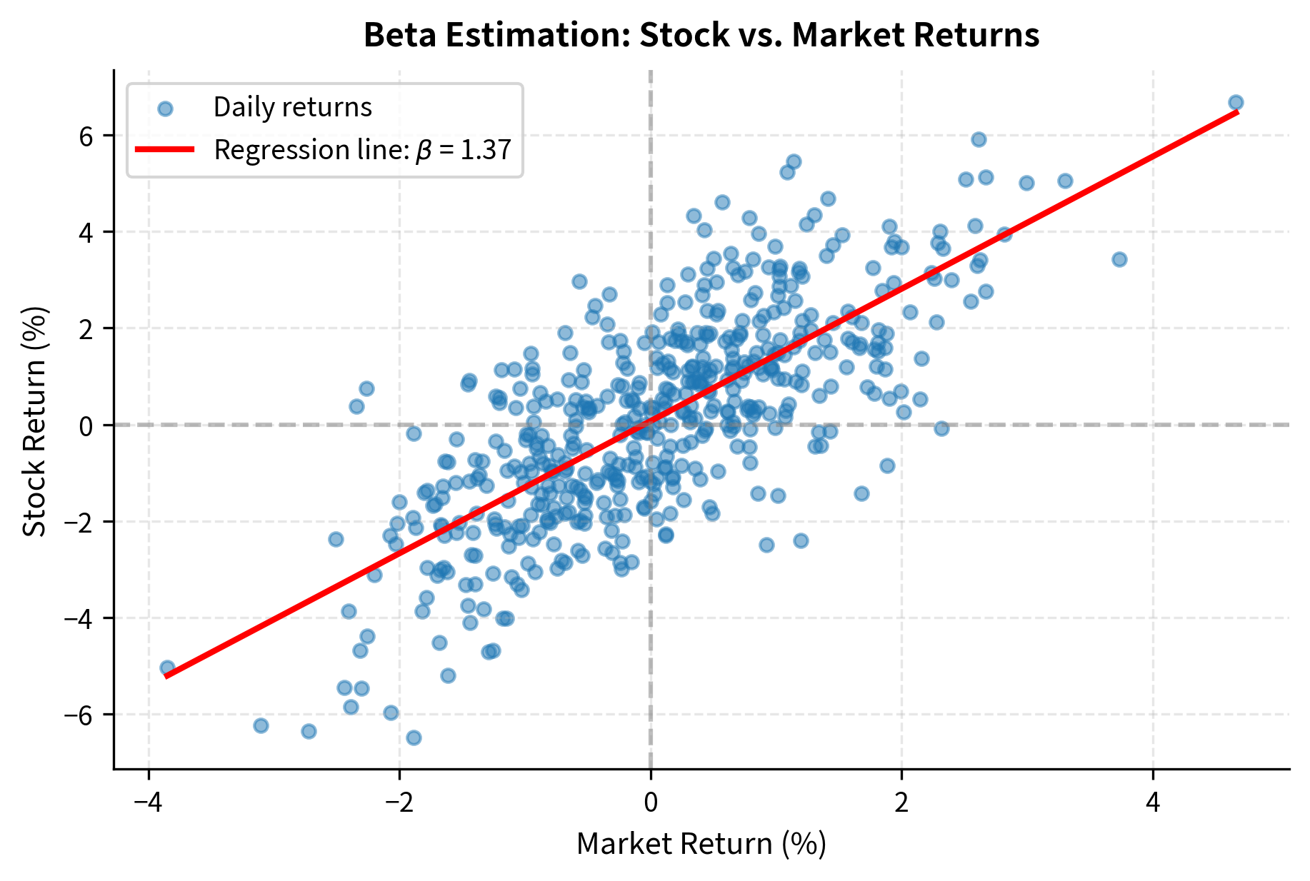
The scatter plot shows that stock returns move in the same direction as market returns but with greater magnitude, consistent with a beta above 1. The stock amplifies market movements by approximately 30%.
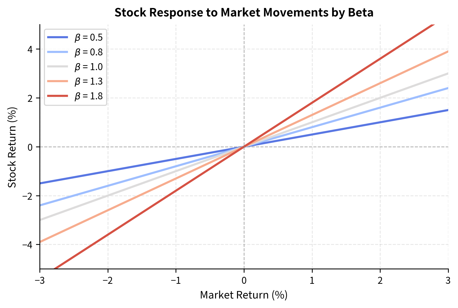
To understand the economic meaning of different beta values, consider how stocks with varying market sensitivities respond to the same market movement:
Hypothesis Testing and Model Evaluation
Estimating coefficients is only the first step. We need to assess whether these estimates are statistically meaningful and how well the model explains variation in the dependent variable. The challenge is that our estimates are random variables: they depend on the particular sample we observed. Different samples would produce different estimates. Statistical inference quantifies this uncertainty, telling us how confident we can be in our conclusions.
Standard Errors and t-Statistics
The uncertainty in coefficient estimates comes from sampling variation. We observe only one realization of the data, but if we could repeatedly sample from the same underlying process, we would get different coefficient estimates each time. The distribution of these hypothetical estimates determines how confident we can be in any single estimate.
Under the classical OLS assumptions (which we'll examine shortly), the coefficient estimates follow a multivariate normal distribution:
where:
- : estimator vector
- : true coefficient vector
- : variance of the error term
- : inverse of the moment matrix of regressors
This result tells us that OLS estimates are unbiased: their expected value equals the true parameter. The covariance matrix determines the precision of each estimate. The diagonal elements give the variances of individual coefficients, while off-diagonal elements capture how estimation errors in different coefficients relate to each other.
Since we don't know , we estimate it using the residual variance:
where:
- : estimated variance of the error term
- : residual for observation
- : sum of squared residuals
- : number of observations
- : number of explanatory variables (excluding intercept)
The denominator accounts for the degrees of freedom lost in estimating parameters (including the intercept). This adjustment ensures the variance estimate is unbiased. With more parameters to estimate, we have less information available to estimate the error variance, so we divide by a smaller number.
The standard error of coefficient is:
where:
- : standard error of the -th coefficient
- : estimated standard deviation of the error term
- : the -th diagonal element of the inverse matrix
The term reflects both the variance of the -th regressor and its correlation with other regressors. High variance in reduces the standard error (more information), while high correlation with other variables increases it (multicollinearity). Intuitively, if a variable moves a lot, we can more precisely estimate its effect. But if it moves together with other variables, it becomes harder to isolate its unique contribution.
To test whether a coefficient differs from zero, we compute the t-statistic:
where:
- : t-statistic for the -th coefficient
- : estimated coefficient
- : standard error of the estimate
This ratio compares the magnitude of the estimate to its precision. A large t-statistic (in absolute value) means the estimate is large relative to its uncertainty, suggesting a genuine non-zero effect. Under the null hypothesis that , this statistic follows a t-distribution with degrees of freedom. The t-distribution accounts for the additional uncertainty from estimating .
Interpreting p-Values
The p-value gives the probability of observing a t-statistic as extreme as or more extreme than the one calculated, assuming the null hypothesis is true. A small p-value (typically below 0.05 or 0.01) suggests the coefficient is statistically significantly different from zero. The logic is indirect: if the null hypothesis were true, the observed result would be very unlikely, so we reject the null.
In financial applications, statistical significance doesn't guarantee economic significance. A beta estimate might be highly significant (p < 0.001) but the relationship might be too weak or unstable to be useful for trading. Conversely, economically meaningful effects might not achieve statistical significance in small samples. The p-value depends on both the magnitude of the effect and the precision of our estimate, so a small but precisely estimated effect can be highly significant while a large but imprecisely estimated effect may not be.
The beta estimate is highly significant, with a t-statistic far exceeding critical values. This means we can confidently reject the null hypothesis that the stock has no market exposure. The alpha estimate, while positive, may or may not be statistically significant depending on the random realization. This illustrates the challenge of detecting true alpha.
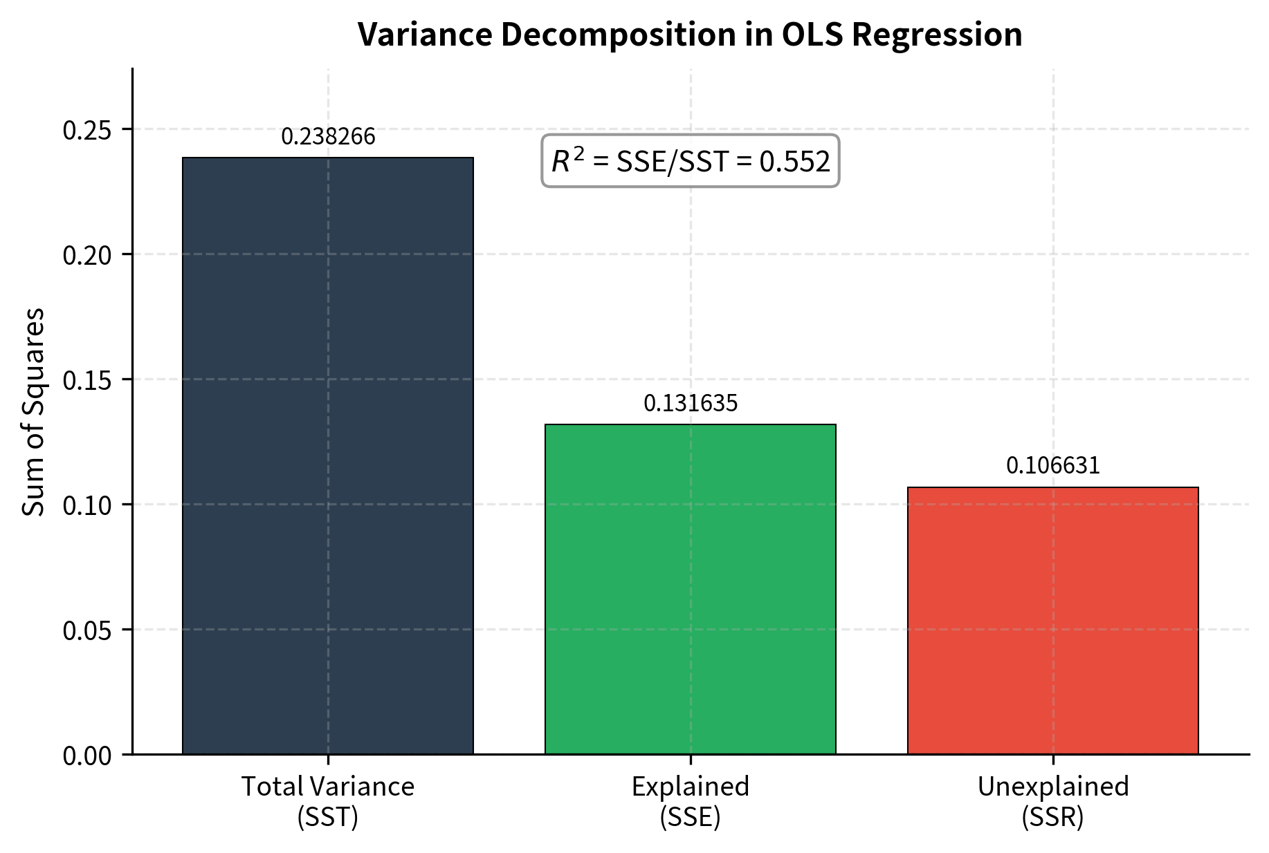
R-Squared: Measuring Fit
The coefficient of determination, , measures the proportion of variance in the dependent variable explained by the model. This statistic answers a fundamental question: how much of the variation in returns can we attribute to the factors in our model, versus unexplained idiosyncratic variation?
where:
- : coefficient of determination
- : sum of squared residuals (unexplained variation)
- : total sum of squares (total variation)
- : observed value of dependent variable
- : fitted value for observation
- : sample mean of the dependent variable
ranges from 0 to 1, with higher values indicating better fit. An of 0.5 means that 50% of the variation in returns is explained by the model, while 50% remains unexplained. The unexplained portion represents idiosyncratic risk and the effects of factors not included in the model.
When comparing models with different numbers of predictors, use adjusted R-squared, which penalizes for adding variables:
where:
- : adjusted coefficient of determination
- : standard coefficient of determination
- : number of observations
- : number of predictors
This prevents overfitting by adding irrelevant predictors that would increase mechanically. The adjustment recognizes that adding any variable, even a random one, will weakly increase . Adjusted can actually decrease if the added variable doesn't improve the model enough to justify the lost degree of freedom.
For single-stock regressions against the market, typically ranges from 0.2 to 0.6 for individual stocks. Lower values indicate more idiosyncratic risk that cannot be diversified through market exposure alone. For portfolios, tends to be higher because idiosyncratic risks cancel out. A well-diversified portfolio might have of 0.9 or higher against the market, indicating that almost all its risk is systematic.
The F-Test for Overall Significance
The F-test assesses whether the model as a whole has explanatory power, meaning whether at least one coefficient (excluding the intercept) is significantly different from zero. While t-tests evaluate individual coefficients, the F-test provides a joint test of all slope coefficients simultaneously. This distinction matters because individual coefficients might be insignificant due to multicollinearity even when the model as a whole explains significant variation.
where:
- : F-statistic for the model
- : total sum of squares
- : sum of squared residuals
- : coefficient of determination
- : number of slope coefficients
- : number of observations
The F-statistic compares the variance explained by the model (per parameter) to the unexplained variance (per degree of freedom). A value significantly greater than 1 indicates the model captures more signal than expected by random chance. The numerator represents average explained variation per variable, while the denominator represents unexplained variation per observation. If the model has no explanatory power, these should be roughly equal, yielding an F-statistic near 1.
Under the null hypothesis that all slope coefficients equal zero, the F-statistic follows an F-distribution with and degrees of freedom.
The highly significant F-statistic confirms that the model explains a statistically significant portion of the variance in stock returns.
For simple regression with one explanatory variable, the F-test is equivalent to the t-test on the slope coefficient (the F-statistic equals the squared t-statistic).
Diagnosing Regression Problems
The validity of OLS inference depends on several assumptions about the error term. With financial time series data, these assumptions are frequently violated, leading to incorrect standard errors and misleading hypothesis tests. Understanding these assumptions and knowing how to detect their violations is essential for producing reliable results. Failing to address these issues can lead to false confidence in spurious relationships or missed opportunities to identify genuine effects.
The Classical Assumptions
The Gauss-Markov assumptions for OLS include:
- Linearity: The relationship between and is linear
- Exogeneity: (errors are uncorrelated with explanatory variables)
- Homoskedasticity: (constant error variance)
- No autocorrelation: for (errors are uncorrelated across observations)
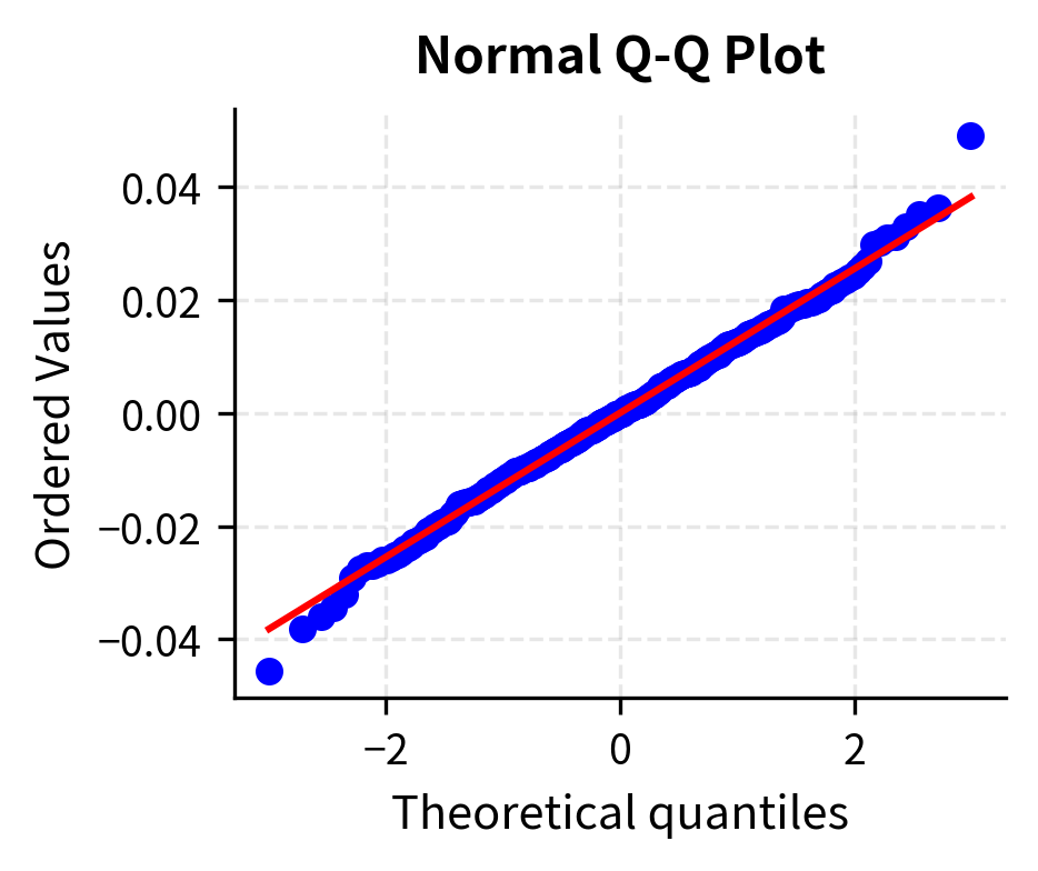
- Normality: (required for exact inference in small samples)
When these assumptions hold, OLS is the Best Linear Unbiased Estimator (BLUE); no other linear unbiased estimator has smaller variance. This optimality result justifies the widespread use of OLS. However, when assumptions are violated, the BLUE property fails, and either the estimates themselves become biased or the standard errors become unreliable.
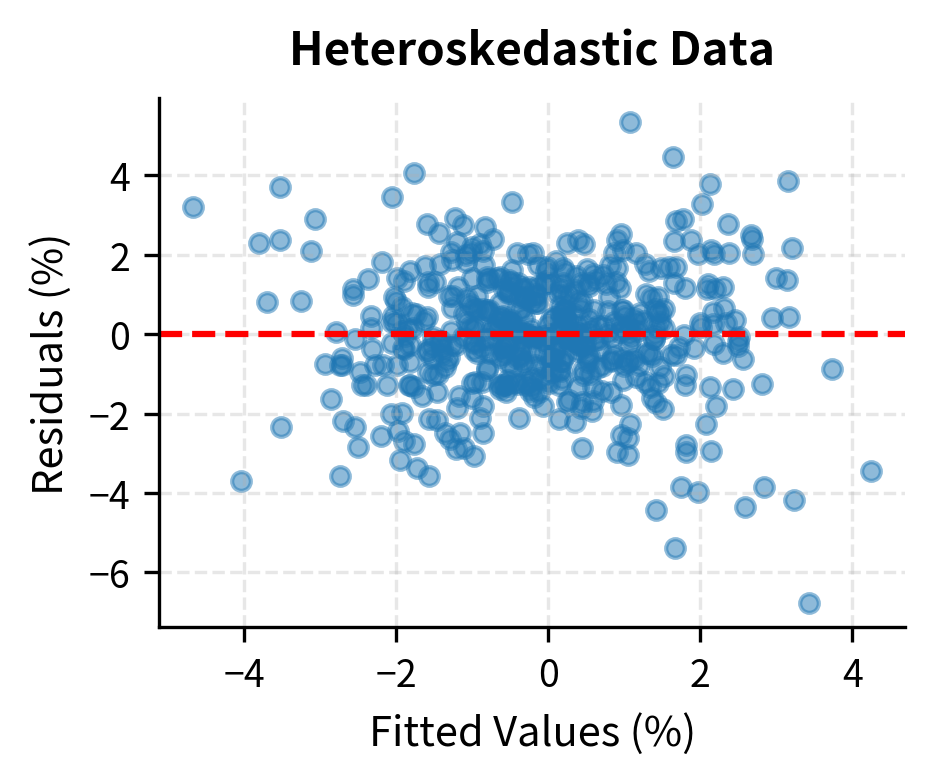
Heteroskedasticity
Heteroskedasticity occurs when the error variance changes across observations. In finance, this is common: volatility varies over time, as we explored in Chapter 18 on GARCH models. Periods of market stress have higher return volatility than calm periods. The variance of returns during the 2008 financial crisis was many times higher than during the calm period of 2005-2006. This time-varying volatility directly translates into heteroskedastic errors in regression models.
Heteroskedasticity doesn't bias the coefficient estimates, but it makes the standard errors incorrect, invalidating hypothesis tests. The OLS formula for standard errors assumes constant variance, so when variance actually varies, these standard errors are wrong. They might be too small (leading to false positives) or too large (leading to false negatives), depending on the pattern of heteroskedasticity.
The Breusch-Pagan test formally tests for heteroskedasticity by regressing squared residuals on the explanatory variables:
The low p-value indicates we reject the null hypothesis of homoskedasticity, confirming the presence of time-varying volatility in our synthetic data.
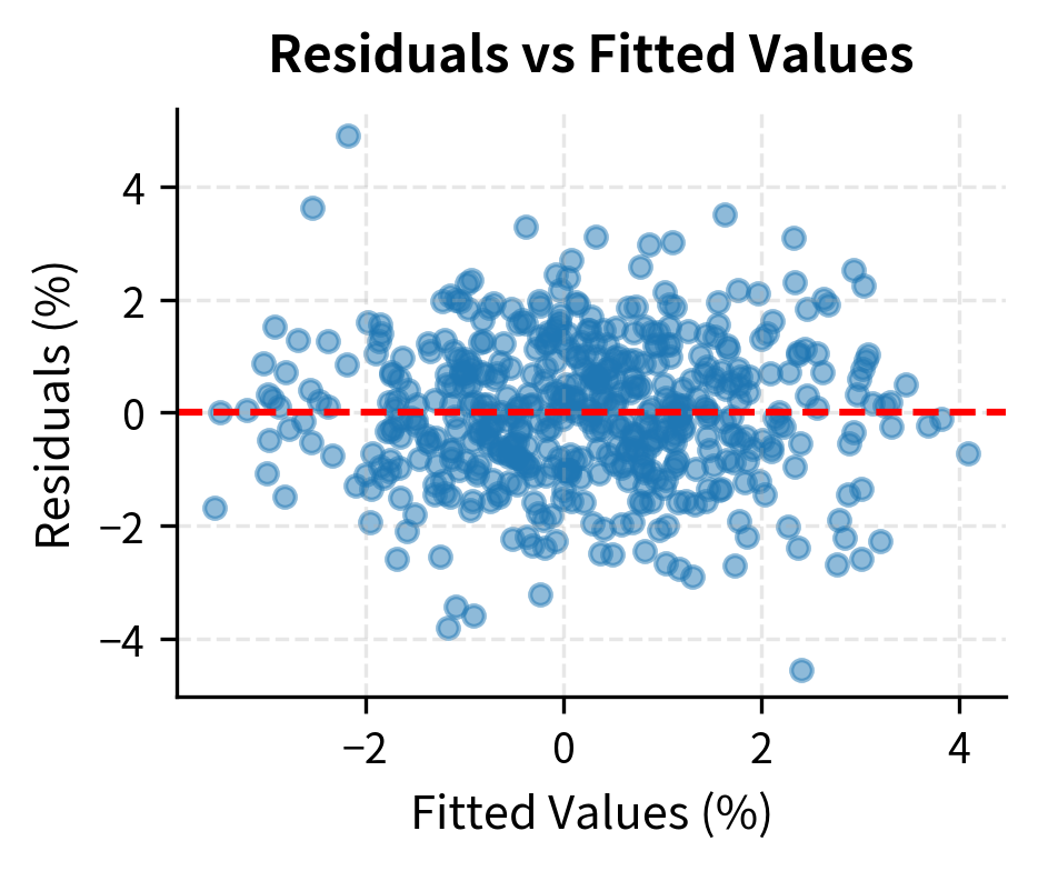
Let's visualize heteroskedasticity by plotting residuals against fitted values:

Autocorrelation
Autocorrelation occurs when errors are correlated across time periods. This is particularly problematic in financial time series because returns often exhibit short-term momentum or mean-reversion patterns in their volatility. When today's error is correlated with yesterday's error, the observations are not truly independent. This reduces the effective sample size: 500 correlated observations contain less information than 500 independent observations.
The Durbin-Watson statistic tests for first-order autocorrelation:
where:
- : Durbin-Watson statistic
- : residual at time
- : number of observations
The numerator sums squared differences between adjacent residuals. If errors are positively correlated, , making the differences small and low (closer to 0). If errors are uncorrelated, the differences are as large as the errors themselves, and the expected value is 2. If errors are negatively correlated, consecutive residuals tend to have opposite signs, making the differences large and high (closer to 4).
Values near 2 indicate no autocorrelation, values below 2 indicate positive autocorrelation, and values above 2 indicate negative autocorrelation.
The Durbin-Watson statistic differs significantly from 2 in the autocorrelated sample, signaling the presence of serial correlation.
We can also examine the autocorrelation function of the residuals:
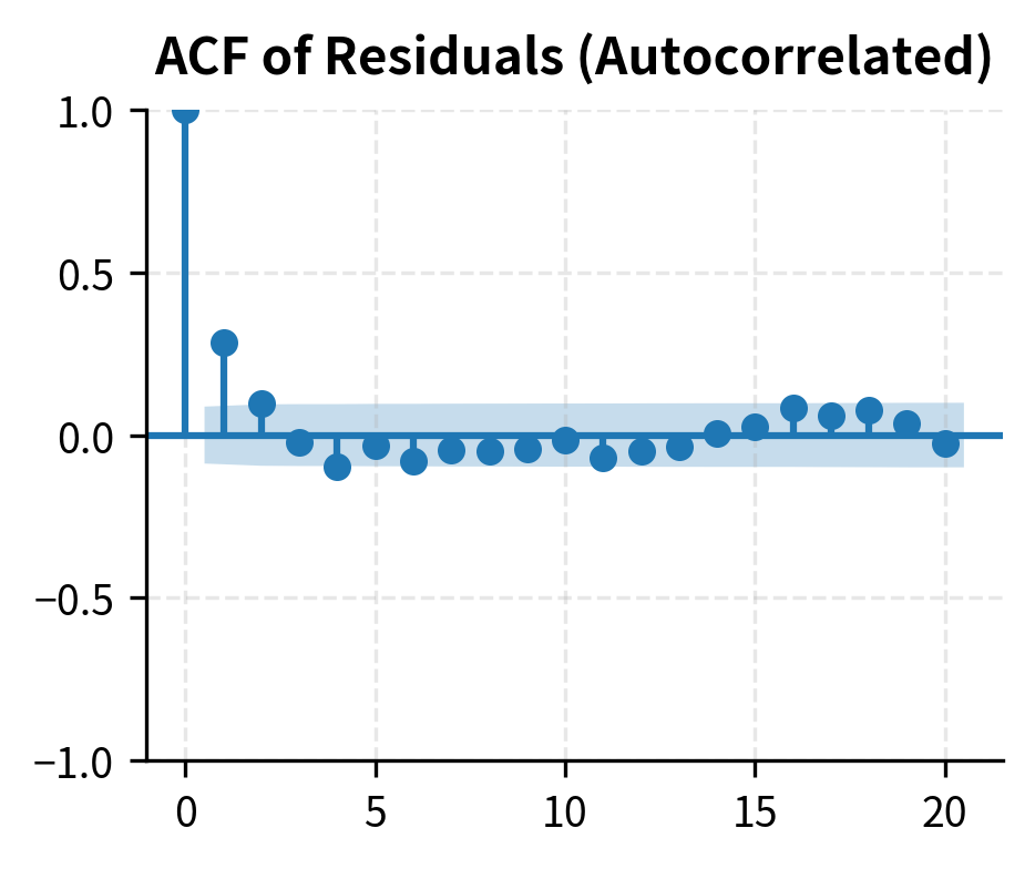
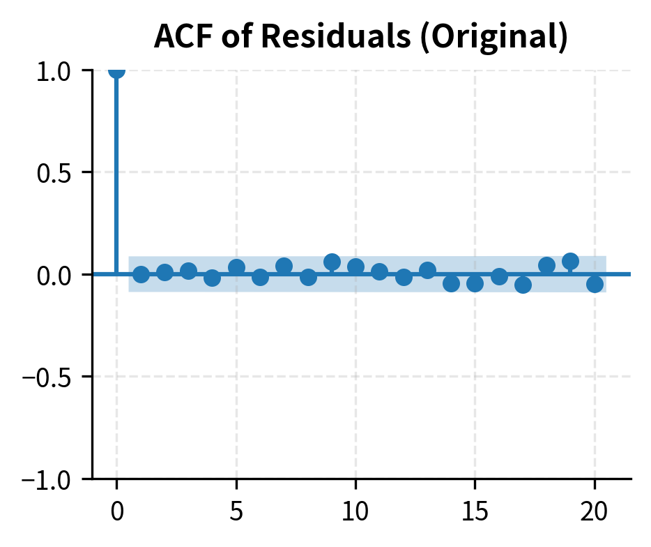
Multicollinearity
Multicollinearity arises when explanatory variables are highly correlated with each other. While not strictly a violation of OLS assumptions, it inflates standard errors and makes coefficient estimates unstable. The fundamental problem is identification: when two variables move together, it becomes difficult to determine which one is driving the effect. Mathematically, the matrix approaches singularity, making its inverse unstable.
The Variance Inflation Factor (VIF) quantifies multicollinearity:
where:
- : Variance Inflation Factor for variable
- : R-squared from regressing variable on all other explanatory variables
If variable is highly correlated with other predictors, approaches 1, causing the denominator to approach zero and to become very large. This mathematically quantifies how much the variance of the estimated coefficient is inflated due to collinearity. A VIF of 5 means the variance is five times what it would be if the variable were uncorrelated with other predictors, making the standard error about 2.2 times larger.
A VIF above 5 or 10 suggests problematic multicollinearity.

Robust Standard Errors
When heteroskedasticity or autocorrelation are present, we can still obtain valid inference by using robust standard errors that don't assume constant variance or independence. These methods adjust the standard error calculation to account for the actual error structure, providing valid confidence intervals and hypothesis tests even when classical assumptions fail. The coefficient estimates themselves remain unbiased; only the uncertainty quantification changes.
Heteroskedasticity-Consistent Standard Errors
White (1980) proposed heteroskedasticity-consistent (HC) standard errors that remain valid even when error variance varies across observations. The idea is to estimate the covariance matrix of using the squared residuals to account for varying error variance. Rather than assuming all errors have the same variance , we allow each observation to have its own variance, estimated by its squared residual.
where:
- : heteroskedasticity-consistent covariance matrix of coefficients
- : matrix of regressors
- : diagonal matrix with squared residuals on the diagonal, accounting for heteroskedasticity
This formula is sometimes called the "sandwich" estimator because the middle term is sandwiched between two copies of . The outer terms handle the variance of the regressors, while the middle term accounts for heteroskedastic errors.
HAC Standard Errors (Newey-West)
For financial time series with both heteroskedasticity and autocorrelation, Newey-West (1987) HAC (Heteroskedasticity and Autocorrelation Consistent) standard errors are the standard approach. These extend the White estimator by also accounting for correlation between errors at different time periods. The key insight is that autocorrelated errors cause cross-products of residuals at different lags to be non-zero, and these must be incorporated into the variance estimate.
where:
- : heteroskedasticity and autocorrelation consistent covariance matrix
- : matrix of regressors
- : estimate of the long-run covariance matrix, accounting for both heteroskedasticity and autocorrelation up to a specified lag
The matrix is computed using a weighted sum of autocovariance matrices at different lags, with weights that decline as the lag increases. This downweighting ensures that distant correlations, which are typically weaker and harder to estimate, have less influence on the variance estimate. The choice of maximum lag (bandwidth) involves a tradeoff: too few lags may miss important autocorrelation, while too many lags reduce precision.
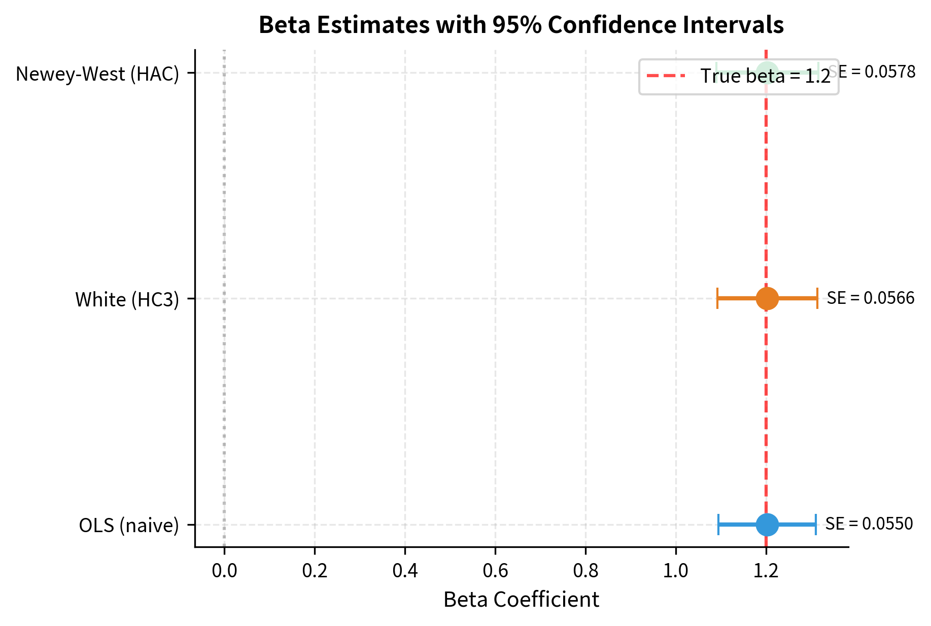
The robust standard errors are typically larger than naive OLS standard errors when autocorrelation is present. This means t-statistics are smaller and p-values are larger, making it harder to reject null hypotheses. This is appropriate: we should be more uncertain about estimates when errors are correlated because we effectively have fewer independent observations. The adjustment prevents us from falsely claiming statistical significance based on overstated precision.
Multiple Regression and Factor Models
While the market model uses a single factor, financial research has established that multiple factors explain cross-sectional return variation. The single-factor CAPM leaves significant patterns unexplained: small stocks earn higher average returns than large stocks, and value stocks (high book-to-market) earn more than growth stocks. These patterns motivated the development of multi-factor models that better capture the systematic risks in equity markets.
The Fama-French three-factor model adds size (SMB: Small Minus Big) and value (HML: High Minus Low) factors:
where:
- : excess return on asset
- : excess return on the market portfolio
- : Small Minus Big size factor, capturing the return premium of small stocks over large stocks
- : High Minus Low value factor, capturing the return premium of value stocks over growth stocks
- : intercept (abnormal return)
- : market beta
- : stock's sensitivity to the size factor
- : stock's sensitivity to the value factor
- : error term
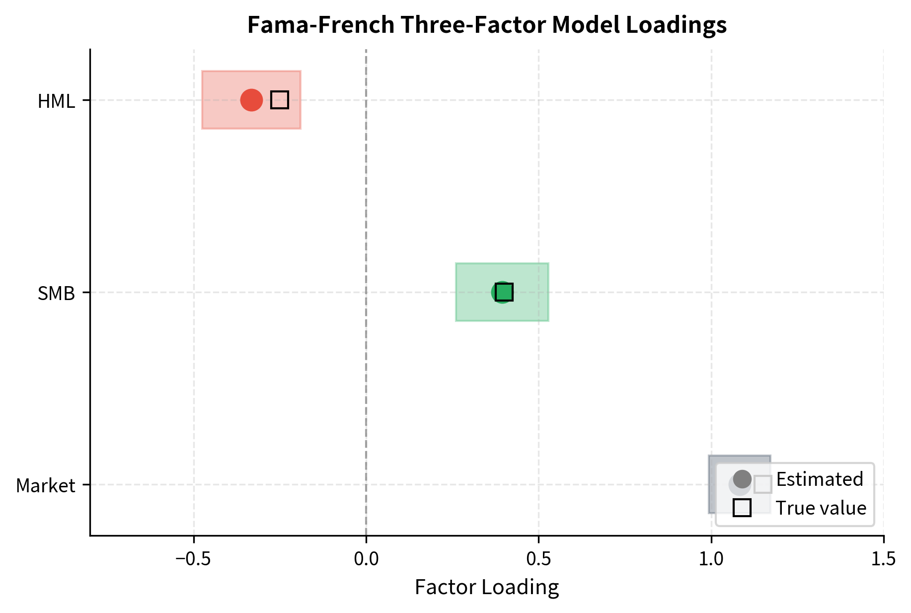
Each coefficient represents exposure to a different systematic risk factor. The market beta captures overall equity market risk. The SMB loading indicates whether the stock behaves more like a small-cap or large-cap stock, regardless of its actual size. The HML loading reveals whether the stock exhibits value or growth characteristics in its return behavior. We'll explore these multi-factor models thoroughly in Part IV when we cover Arbitrage Pricing Theory.
Implementing Multi-Factor Regression
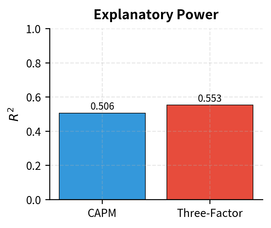
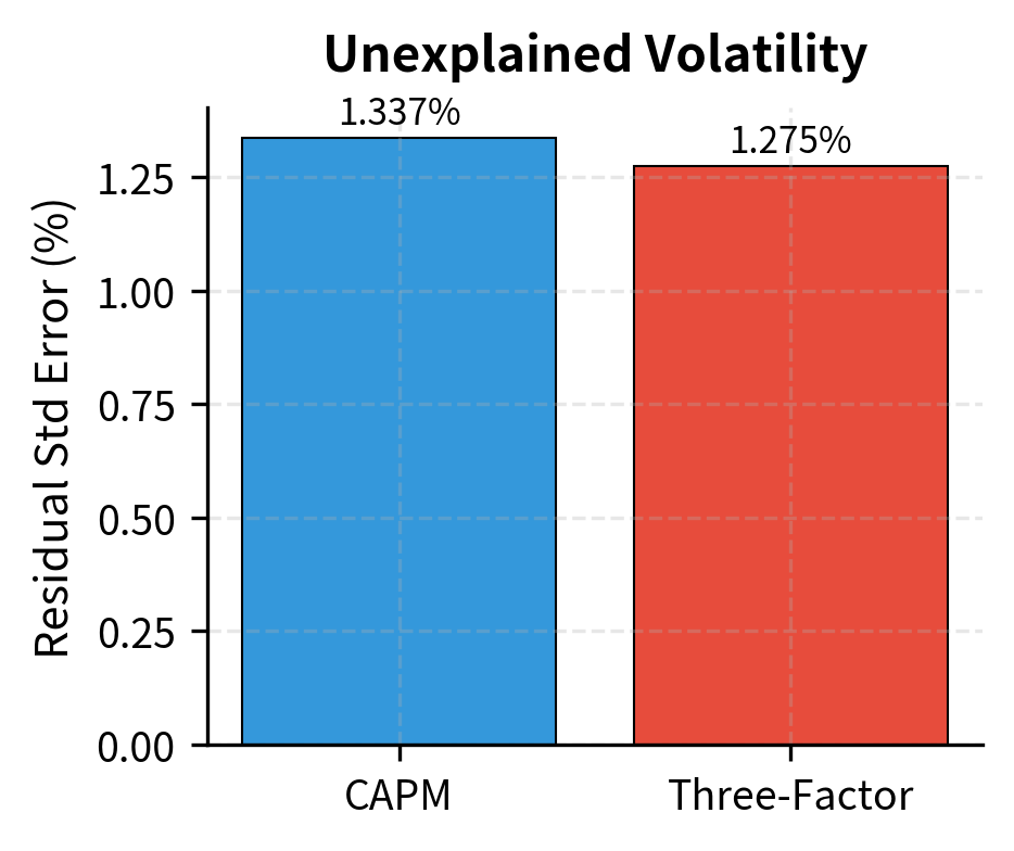
The results show significant exposure to all three factors. The stock has a market beta of approximately 1.15, meaning it's more volatile than the market. The positive SMB loading indicates a tilt toward small-cap characteristics, while the negative HML loading suggests growth rather than value exposure. Adding factors improves the model's explanatory power, as shown by the higher R-squared compared to a single-factor model.
Comparing Single and Multi-Factor Models
A Complete Regression Workflow
Let's demonstrate a complete workflow for estimating and validating a factor model, incorporating all the diagnostic and inference techniques covered.
The diagnostic summary quickly flags potential issues. In this case, we look for "WARNING" flags that would necessitate using robust standard errors or model re-specification.
Key Parameters
The key parameters for regression models in finance are:
- y: Dependent variable (e.g., stock returns). The target variable to be explained.
- X: Independent variables (factors). The explanatory variables such as market returns.
- : Intercept (Alpha). Measures abnormal performance not explained by factors.
- : Slope (Beta). Measures systematic risk or sensitivity to a factor.
- : Error term. Captures idiosyncratic risk and unexplained variation.
- : R-squared. Indicates the proportion of variance explained by the model.
Limitations and Practical Considerations
Regression analysis is a powerful tool, but its proper application in finance requires understanding several limitations and pitfalls.
The stationarity assumption underlying OLS may be violated in financial applications. Beta estimates, for instance, are not constant through time, as a stock's sensitivity to the market can change as the company grows, changes industries, or faces different competitive pressures. Rolling-window regressions or time-varying parameter models can address this, but the fundamental issue remains: historical relationships may not persist into the future. This is why professional risk managers often blend statistical estimates with fundamental judgment.
The look-ahead bias problem plagues many regression applications in backtesting. If you use data from the entire sample period to estimate betas, then evaluate performance using those same betas, you've implicitly used future information. Proper out-of-sample testing requires estimating parameters only with data available at each point in time, such as through a rolling or expanding window approach. Factor exposures estimated with complete sample data almost always look better than what would have been achievable in real-time.
Omitted variable bias occurs when relevant explanatory variables are excluded from the regression. If an omitted variable is correlated with both the dependent variable and included explanatory variables, coefficient estimates will be biased. This is why CAPM alpha estimates often shrink or disappear when additional factors are included: what looked like skill was actually exposure to priced factors not in the model.
Measurement error in explanatory variables causes attenuation bias: coefficients biased toward zero. Financial data often contains measurement issues: prices might include stale quotes, returns might be calculated from non-synchronous data, and accounting data has reporting lags. Errors-in-variables models and instrumental variable techniques can address this, but they require additional assumptions and data.
Despite these limitations, regression analysis remains foundational because it provides a systematic framework for decomposing returns into explained and unexplained components, testing hypotheses about relationships, and making the uncertainty in our estimates explicit through confidence intervals and p-values. The key is to use regression as a tool for understanding rather than as a black box: always checking assumptions, validating results out-of-sample, and interpreting findings in economic context.
Summary
This chapter developed regression analysis as the primary tool for understanding relationships between financial variables. We covered:
-
The OLS framework provides closed-form estimates for linear relationships. The slope coefficient measures the change in the dependent variable for a unit change in the explanatory variable, while the intercept captures the baseline level.
-
Factor exposures and beta quantify systematic risk. In the market model, beta measures an asset's sensitivity to market movements, which is the foundation for the CAPM that we'll explore in Part IV.
-
Hypothesis testing assesses whether relationships are statistically significant. T-tests evaluate individual coefficients, F-tests assess overall model significance, and R-squared measures explanatory power.
-
Diagnostic tests reveal violations of OLS assumptions. The Durbin-Watson test detects autocorrelation, the Breusch-Pagan test identifies heteroskedasticity, and VIF measures multicollinearity.
-
Robust standard errors (HAC/Newey-West) provide valid inference when classical assumptions fail. These are essential for financial time series data where volatility clusters and returns may be serially correlated.
-
Multiple regression extends the framework to multiple factors, decomposing returns into exposures to market, size, value, and other systematic factors.
The techniques developed here will serve as building blocks for the upcoming chapters. In Chapter 20, we'll use Principal Component Analysis to extract factors from return data rather than specifying them a priori. Part IV will apply these regression tools extensively to estimate and test asset pricing models, measure portfolio performance, and attribute returns to different sources.
Quiz
Ready to test your understanding? Take this quick quiz to reinforce what you've learned about regression analysis for financial relationships.

Comments