

Learn PCA for extracting factors from yield curves and equity returns. Master dimension reduction, eigendecomposition, and risk decomposition techniques.
Choose your expertise level to adjust how many terms are explained. Beginners see more tooltips, experts see fewer to maintain reading flow. Hover over underlined terms for instant definitions.
Principal Component Analysis and Factor Extraction
Financial markets generate vast amounts of correlated data. If you track 500 stocks, you observe 500 time series of returns, yet these returns don't move independently. They share common drivers: the overall market, sector trends, interest rate movements, and macroeconomic forces. Similarly, if you monitor a yield curve across 30 maturities, you don't observe 30 independent interest rates. Instead, a handful of underlying factors, commonly interpreted as the level, slope, and curvature of the yield curve, explain the vast majority of yield movements.
Principal Component Analysis (PCA) provides a systematic way to extract these underlying factors from high-dimensional data. It transforms a set of correlated variables into a smaller set of uncorrelated components that capture most of the variation in the original data. This dimension reduction serves multiple purposes in quantitative finance: it simplifies risk modeling by identifying the dominant sources of portfolio variance, it enables efficient hedging by revealing which instruments move together, and it provides interpretable factors that explain asset price behavior.
The technique rests on the linear algebra concepts we covered in Part I. Specifically, PCA exploits the eigendecomposition of covariance matrices to find orthogonal directions of maximum variance. By projecting data onto these directions, we distill the essential information from dozens or hundreds of variables into a manageable number of factors.
This chapter develops the mathematical foundations of PCA, demonstrates its application to yield curves and equity returns, and connects it to the broader framework of factor models that we'll explore further in Part IV.
The Need for Dimension Reduction
High-dimensional financial data creates practical challenges that dimension reduction addresses. Before diving into the mathematical machinery of PCA, it helps to understand the fundamental problem we are trying to solve. When we observe many correlated financial variables, we are not really looking at independent pieces of information. Instead, we are seeing multiple manifestations of a smaller number of underlying forces. Recognizing this structure allows us to work with the essential drivers rather than the noisy surface observations.
Consider building a covariance matrix for risk management. With assets, the covariance matrix contains unique elements. This formula arises because the covariance matrix is symmetric: the covariance between asset and asset equals the covariance between asset and asset . We therefore need to estimate only the diagonal entries (the variances) plus the entries above the diagonal (which number ). For 500 stocks, that's 125,250 parameters to estimate. With typical sample sizes of a few years of daily data (roughly 750 observations), we face severe estimation error. The resulting covariance matrix may not even be positive definite, rendering it unusable for optimization.
The curse of dimensionality refers to the phenomenon where statistical estimation becomes unreliable as the number of parameters grows relative to sample size. In finance, this manifests when the number of assets approaches or exceeds the number of time periods available for estimation.
PCA addresses this by recognizing that the true dimensionality of asset returns is much lower than the number of assets. If a small number of common factors drive most return variation, we can model the covariance structure using far fewer parameters. For instance, if three factors explain 90% of yield curve variance, we can characterize the term structure's behavior through just three components rather than dozens of individual yields. This insight transforms an intractable estimation problem into a manageable one, allowing us to build reliable risk models even when the number of assets is large relative to our sample size.
The benefits extend beyond numerical stability:
- Interpretability: Principal components often correspond to economically meaningful factors. In yield curves, the first three components map to intuitive concepts of parallel shifts, steepening/flattening, and curvature changes. This interpretability helps bridge the gap between statistical analysis and economic understanding.
- Noise reduction: By discarding components that explain little variance, PCA filters out idiosyncratic noise and reveals the systematic structure in data. The components we discard are dominated by estimation error and random fluctuations rather than meaningful signal.
- Hedging efficiency: Understanding that a few factors drive most variation allows you to hedge broad exposures with a small number of instruments. Rather than trading all 30 points on a yield curve, you can focus on positions in a handful of key maturities that span the principal components.
Mathematical Foundation of PCA
PCA transforms a set of correlated variables into uncorrelated principal components, ordered by the amount of variance they explain. The transformation is linear and orthogonal, meaning it preserves distances and angles while rotating the coordinate system to align with directions of maximum variance. This section develops the mathematical framework that makes this transformation possible, starting from the raw data and building toward the eigenvalue problem that lies at the heart of PCA.
Setting Up the Problem
Suppose we have observations of variables, organized in an data matrix . Each row represents one observation (e.g., one day's yield curve), and each column represents one variable (e.g., the yield at a specific maturity). This matrix structure provides a natural way to organize our data: reading across a row shows us the complete cross-section of variables at one point in time, while reading down a column reveals the time series of a single variable.
The first step is to center the data by subtracting the column means. Centering is essential because PCA seeks directions of maximum variance, and variance is measured relative to the mean. Without centering, the first principal component would simply point toward the overall mean of the data rather than capturing the directions of greatest spread. Let denote the -dimensional vector of column means. The centered data matrix is:
where:
- : centered data matrix
- : original data matrix
- : vector of ones of size
- : vector of column means
In this expression, the outer product creates an matrix where every row is identical to the transpose of the mean vector. Subtracting this from the original data ensures that each column of the resulting matrix has mean zero.
The sample covariance matrix is then:
where:
- : sample covariance matrix
- : number of observations
- : centered data matrix
To understand why this formula produces the covariance matrix, consider what happens when we multiply by . The result is a matrix where the entry equals the sum of products of the centered values for variables and across all observations. Dividing by (rather than ) gives us the unbiased sample covariance, correcting for the fact that we have estimated the means from the same data. This symmetric positive semi-definite matrix captures how the variables co-move. The diagonal elements are variances; the off-diagonal elements are covariances.
Eigendecomposition and Principal Components
As we discussed in Part I's treatment of linear algebra, any symmetric matrix can be decomposed into its eigenvalues and eigenvectors. This spectral theorem is the mathematical foundation of PCA, providing the key insight that allows us to find orthogonal directions of maximum variance. For the covariance matrix:
where:
- : covariance matrix
- : diagonal matrix of eigenvalues
- : orthogonal matrix of eigenvectors
- : -th eigenvector (column of )
- : total number of variables
The eigenvalues are ordered from largest to smallest, reflecting the importance of each direction for explaining variance. Because the covariance matrix is positive semi-definite (a property inherited from its construction as scaled by a positive constant), all eigenvalues are non-negative. The eigenvectors form an orthonormal basis, meaning they are mutually perpendicular and each has unit length. This orthogonality is crucial because it ensures that the principal components are uncorrelated.
The -th principal component is defined as the projection of the centered data onto the -th eigenvector:
where:
- : vector of scores for the -th principal component
- : centered data matrix
- : -th eigenvector (loading vector)
This projection operation computes a weighted sum of the original variables for each observation, where the weights come from the eigenvector. The result is an -dimensional vector of principal component scores, with one score for each observation. The eigenvector is called the -th loading vector because it specifies how each original variable contributes to the component. A large positive loading means that variable contributes strongly and positively to the component; a large negative loading means it contributes strongly but in the opposite direction.
Why Eigendecomposition Maximizes Variance
The first principal component is the linear combination of the original variables with maximum variance. This is not merely a convenient property but rather the defining characteristic of PCA. To see why finding this direction of maximum variance corresponds to finding the first eigenvector, consider finding the unit vector that maximizes the variance of .
The variance of the projection is:
where:
- : projection vector (weights)
- : covariance matrix
- : centered data matrix
- : number of observations
This derivation reveals a key connection: the variance of any linear combination of our variables equals a quadratic form in the covariance matrix. The quadratic form measures how the covariance structure "stretches" the unit vector . Our goal is to find the direction that experiences maximum stretching.
We want to maximize this subject to . The constraint is necessary because without it, we could increase variance indefinitely by scaling . By restricting ourselves to unit vectors, we focus on finding the direction of maximum variance rather than an arbitrarily long vector. Using Lagrange multipliers (recall our optimization discussion from Part I), we set:
where:
- : Lagrangian function
- : Lagrange multiplier (eigenvalue)
- : projection vector
- : covariance matrix
The Lagrangian incorporates our constraint through the multiplier , which will turn out to have a deep interpretation as the eigenvalue. Taking the derivative with respect to and setting it to zero:
where:
- : gradient of the Lagrangian with respect to
- : covariance matrix
- : projection vector
- : Lagrange multiplier (eigenvalue)
The gradient of the quadratic form equals because of the symmetry of , and the gradient of equals . This yields the eigenvalue equation:
where:
- : covariance matrix
- : eigenvector
- : eigenvalue
This equation has a geometric interpretation. The covariance matrix acts as a linear transformation that stretches and rotates vectors. An eigenvector is special because when acts on it, the result points in the same direction as the original vector, merely scaled by the eigenvalue . These are precisely the directions along which the covariance structure exhibits pure stretching without rotation.
Substituting this into the variance definition:
where:
- : variance of the projected data
- : projection vector
- : covariance matrix
- : eigenvalue
This result shows that the variance of the projection onto an eigenvector exactly equals the corresponding eigenvalue. To maximize variance, we choose the eigenvector with the largest eigenvalue. This eigenvector points in the direction of greatest spread in our data.
For subsequent components, we impose the additional constraint of orthogonality to previously selected directions. This sequential optimization produces the full set of eigenvectors, ordered by decreasing eigenvalue. The second principal component is the direction of maximum variance among all directions perpendicular to the first, and so on. Because the eigenvectors of a symmetric matrix are automatically orthogonal, the eigendecomposition provides exactly what we need.
Variance Explained
The eigenvalues have a direct interpretation: equals the variance of the -th principal component. This is not a coincidence but follows directly from the derivation above. When we project our data onto the -th eigenvector, the resulting variance equals . The total variance in the data equals the sum of all eigenvalues (which also equals the trace of the covariance matrix):
where:
- : -th eigenvalue (variance of -th component)
- : trace of the covariance matrix
- : total number of variables
This identity reflects a fundamental property of the eigendecomposition: the trace of a matrix (the sum of its diagonal elements) equals the sum of its eigenvalues. Since the diagonal elements of the covariance matrix are the variances of individual variables, the total variance is conserved when we rotate to the principal component basis. PCA does not create or destroy variance; it merely redistributes it across orthogonal directions.
The proportion of variance explained by the first components is:
where:
- : cumulative proportion of variance explained
- : number of retained components
- : variance of the -th component
- : total number of variables
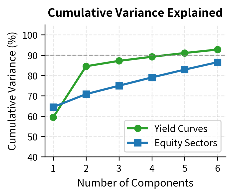
This metric guides the choice of how many components to retain. In financial applications, it's common to retain enough components to explain 90-95% of variance, though the appropriate threshold depends on the application. For yield curve modeling, where the first three components typically explain over 99% of variance, the choice is clear. For equity returns, where variance is more dispersed, the decision requires more judgment about the tradeoff between parsimony and fidelity.
Implementing PCA from Scratch
Let's implement PCA step by step to solidify the mathematical concepts. We'll use a simple example before moving to financial applications.
Now we center the data and compute the covariance matrix:
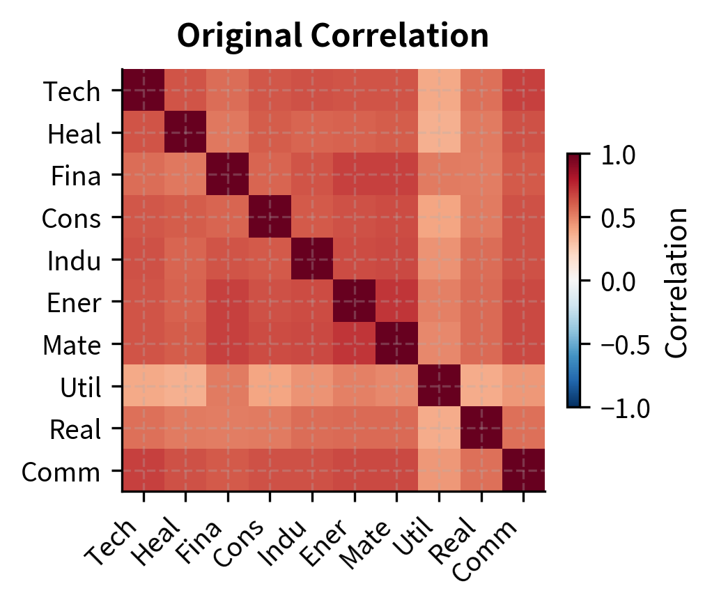
The covariance matrix shows strong positive correlations among all three variables, consistent with a common factor structure.
Next, we compute eigenvalues and eigenvectors:
The first principal component captures the dominant common movement across all three variables, explaining about 85% of total variance. The second captures most of the remaining variance, leaving very little for the third. This confirms that our three observed variables are effectively driven by two underlying factors.
The eigenvectors (loading vectors) tell us how each original variable contributes to each component:
The first component has positive loadings on all variables, representing their common factor. The second component has loadings of opposite signs, capturing the differential between certain variables. This corresponds to the second factor in our data-generating process.
Finally, we project the data onto the principal components:
The principal components are uncorrelated by construction, and their standard deviations equal the square roots of the corresponding eigenvalues.
PCA Applied to Yield Curves
The term structure of interest rates provides one of the most compelling applications of PCA in finance. As we discussed in Part II when covering bond pricing and the term structure, yield curves across maturities move together in systematic ways. PCA extracts the dominant patterns of yield curve movements.
Simulating Yield Curve Data
We'll simulate realistic yield curve data based on the well-documented empirical patterns of level, slope, and curvature movements:
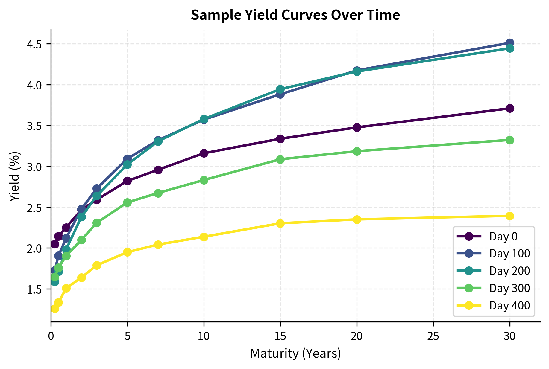
Let's visualize several yield curves from our simulated data:
The yield curves show the typical upward slope with variations in their overall level, steepness, and curvature. This is exactly what our three factors produce.
Applying PCA to Yield Changes
In practice, we usually apply PCA to yield changes rather than yield levels because changes are more stationary. This follows the same logic as our discussion of returns versus prices in the time series chapter.
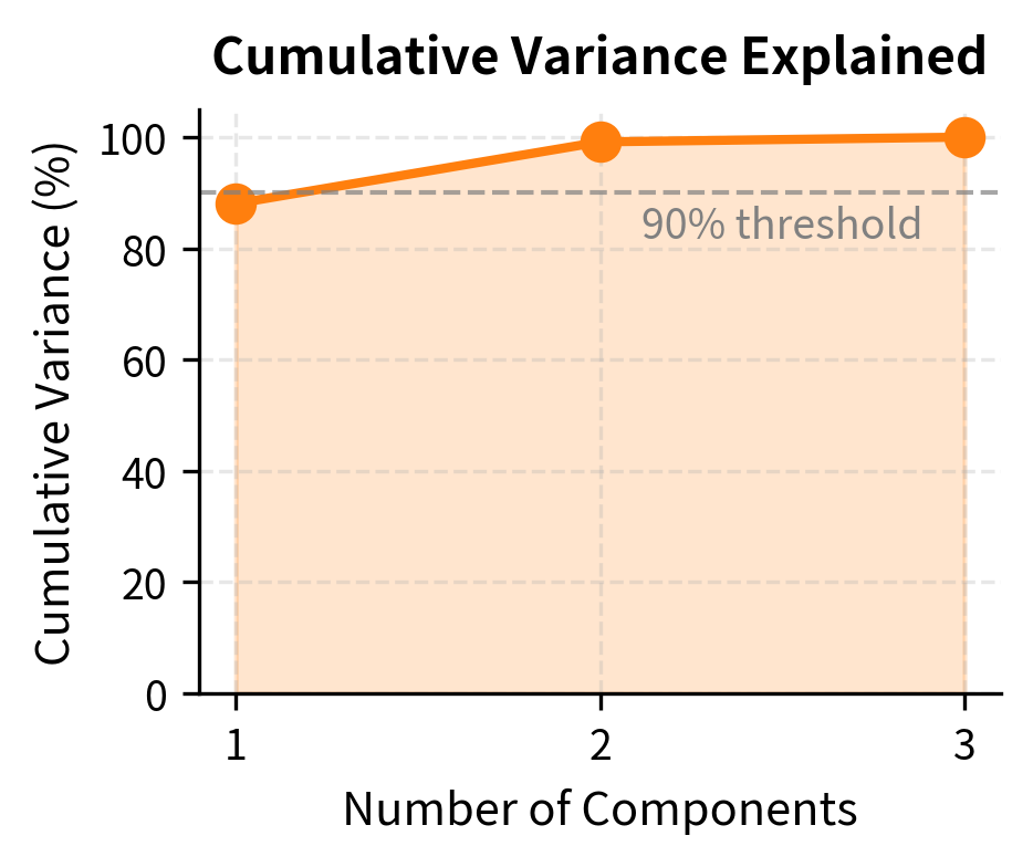
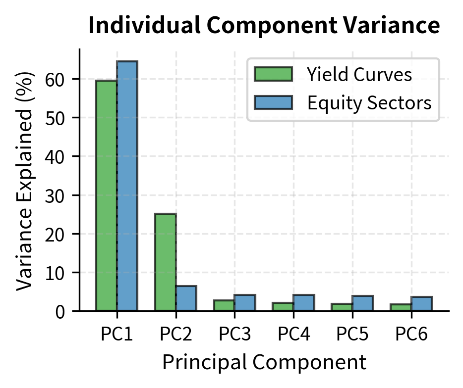
The first three principal components explain over 99% of yield curve variation, confirming the well-known empirical result that yield curves have very low effective dimensionality. This finding has practical implications: despite having 11 maturities, we can capture virtually all yield curve dynamics with just three factors.
Interpreting the Principal Components
The loading vectors reveal the economic interpretation of each component:

The three components have clear economic interpretations:
-
PC1 (Level): Nearly constant loadings across maturities. When this component increases, all yields move up by similar amounts, representing a parallel shift of the entire curve.
-
PC2 (Slope): Loadings change monotonically with maturity, positive at one end and negative at the other. A positive shock to this component steepens the curve (short rates fall while long rates rise, or vice versa).
-
PC3 (Curvature): Loadings peak at intermediate maturities with opposite signs at the extremes. This component captures "twist" movements where the middle of the curve moves differently from the ends.
These interpretations are consistent across different countries, time periods, and yield curve datasets. The level factor typically explains 80-90% of variance, slope explains 5-10%, and curvature explains most of the remainder.
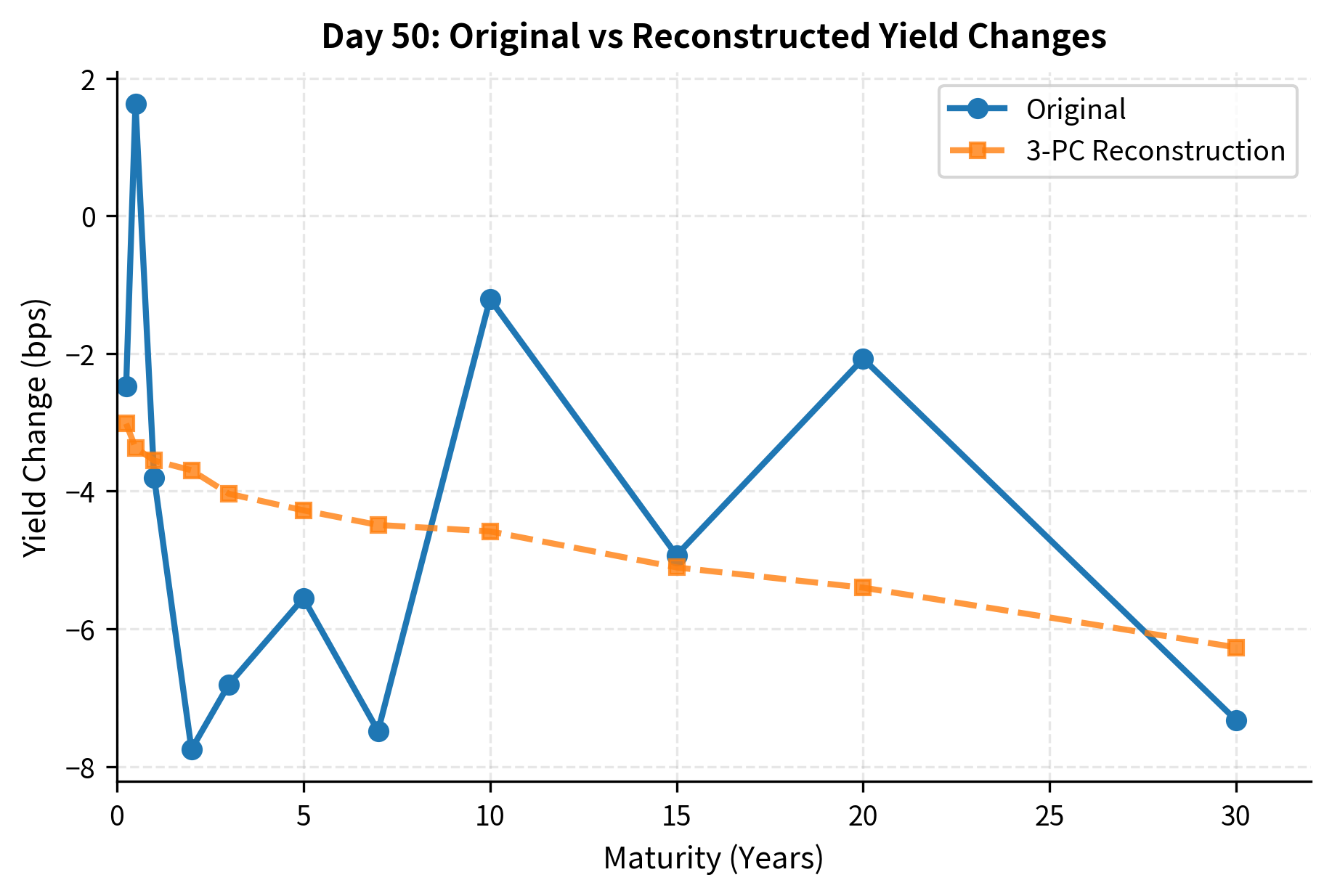
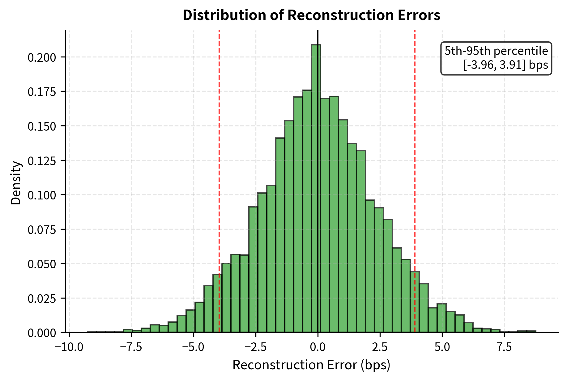
Reconstructing Yield Curves
We can reconstruct yield curve changes using only the first few principal components. This demonstrates how dimension reduction works in practice:
The reconstruction error is tiny compared to the magnitude of yield changes, confirming that three components capture the essential dynamics.
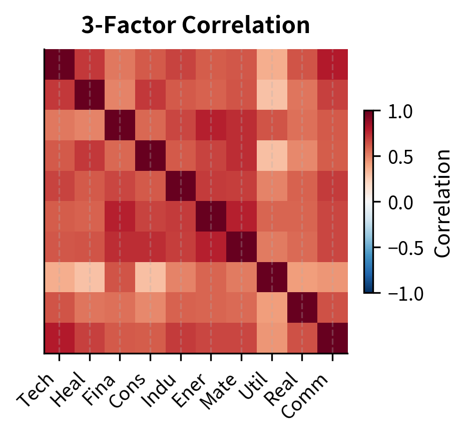
PCA Applied to Equity Returns
Equity returns present a more challenging application of PCA. Unlike yield curves, where maturities have a natural ordering and the factor structure is highly regular, equity returns exhibit a messier factor structure with lower variance concentration in the leading components.
Analyzing Sector Returns
Let's apply PCA to a set of simulated sector returns:
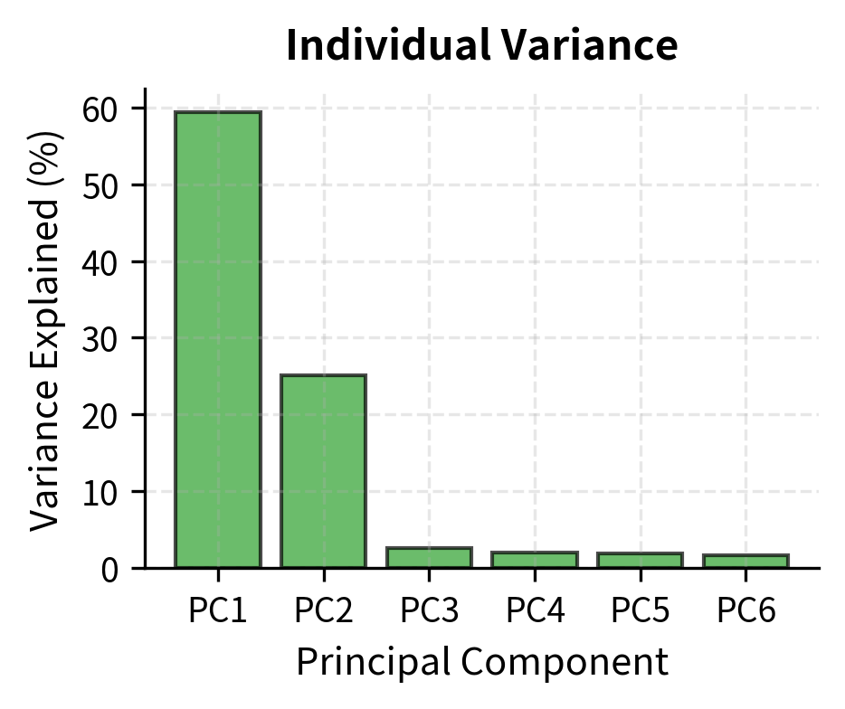
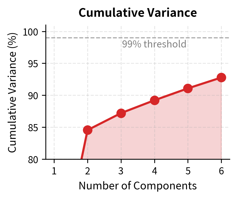
Unlike yield curves, equity returns require more components to achieve high variance explanation. The first component (the market factor) explains a smaller fraction of total variance because idiosyncratic risk is more significant for individual stocks and sectors.
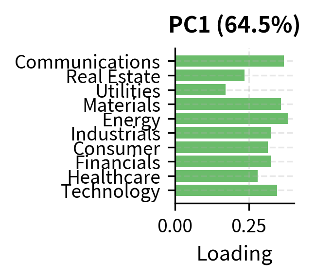
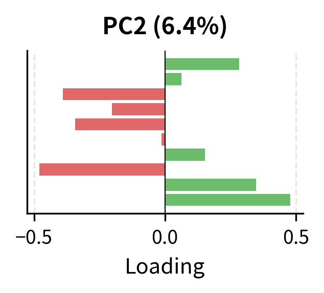
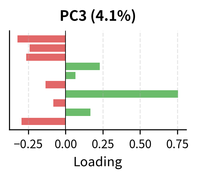
The loading patterns reveal the underlying factor structure:
- PC1: All positive loadings indicate a common market factor. The relative magnitudes reflect each sector's market beta.
- PC2: The pattern of positive and negative loadings separates sectors along a dimension that might correspond to growth versus value characteristics.
- PC3: Further differentiation, potentially capturing interest rate sensitivity given the high loadings on Utilities and Real Estate.
Using scikit-learn for PCA
For production applications, scikit-learn provides an efficient and well-tested PCA implementation:
The output confirms that the first few principal components capture the majority of the variance, consistent with our manual implementation. However, the exact percentages differ slightly because we standardized the data. Standardization effectively performs PCA on the correlation matrix (giving equal weight to all assets) rather than the covariance matrix (where high-volatility assets dominate).
When variables have different scales, standardizing them (subtracting the mean and dividing by standard deviation) before PCA ensures that all variables contribute equally to the analysis. For yield curves, where all variables are in the same units (percentage yields), standardization is typically unnecessary. For equity returns with different volatilities, standardization may be appropriate depending on whether you want to explain variance in original units or give equal weight to all assets.
Key Parameters
The key parameters for Principal Component Analysis are:
- X: The input data matrix of shape , where is the number of observations and is the number of variables.
- n_components: The number of principal components to retain. This determines the dimensionality of the reduced data.
- Standardization: Whether to scale variables to unit variance before analysis. This is critical when variables have different units or vastly different variances.
- Centering: PCA requires data to be centered (mean zero). This is handled automatically by most libraries but is a necessary preprocessing step in manual implementation.
Connection to Factor Models
PCA extracts statistical factors from data without imposing any economic structure. This contrasts with economic factor models like CAPM and APT, which we'll study in Part IV. Understanding the relationship between these approaches is crucial for quantitative practice. Both approaches seek to explain asset returns through a small number of common factors, but they differ fundamentally in how those factors are identified and what guarantees they provide.
Statistical versus Fundamental Factors
Factor models express asset returns as linear combinations of factor exposures:
where:
- : return on asset
- : intercept (alpha) for asset
- : factor loading of asset on factor
- : return of factor
- : idiosyncratic return
- : number of factors
This linear structure assumes that each asset's return can be decomposed into two parts. The systematic component, captured by the summation term, reflects the asset's exposure to common factors. The idiosyncratic component represents asset-specific fluctuations uncorrelated with the factors or with other assets' idiosyncratic terms.
The factors can be:
-
Fundamental/Economic: Observable characteristics like market returns, size, value, momentum. These have clear economic interpretations but require us to specify them in advance. You must decide which factors to include based on economic theory or empirical evidence.
-
Statistical: Extracted from return data using techniques like PCA. These are guaranteed to be uncorrelated and to maximize variance explanation, but their economic interpretation must be inferred after extraction. PCA does not tell us what the factors represent; it only tells us that they capture the dominant patterns in the data.
PCA provides the optimal statistical factors in the sense that no other set of orthogonal factors can explain more variance. However, statistical factors may not correspond to tradeable portfolios or have stable interpretations over time. The first principal component of equity returns resembles the market factor, but subsequent components often lack clear economic meaning and may shift as the composition of the market changes.
PCA and the Covariance Matrix
A key insight connects PCA to portfolio risk management. The covariance matrix decomposition:
where:
- : covariance matrix
- : orthogonal matrix of eigenvectors
- : diagonal matrix of eigenvalues
- : -th eigenvalue
- : -th eigenvector
- : total number of variables
This representation expresses the covariance matrix as a sum of outer products, where each term is a rank-one matrix scaled by the corresponding eigenvalue. The decomposition shows that the covariance matrix is a weighted sum of rank-one matrices, with weights given by eigenvalues. This has practical implications:
-
Factor risk decomposition: The total variance of any portfolio can be decomposed into contributions from each principal component. This allows you to identify which systematic factors drive portfolio volatility and to understand whether risk is concentrated in one factor or spread across many.
-
Regularization: For ill-conditioned covariance matrices (common with many assets and limited data), we can improve estimation by shrinking small eigenvalues or discarding noisy components. Small eigenvalues are most affected by estimation error, and setting them to zero or a small positive value can dramatically improve the stability of downstream calculations like portfolio optimization.
-
Scenario analysis: We can stress test portfolios by shocking individual principal components, which represent the orthogonal sources of systematic risk. A one-standard-deviation shock to the first principal component simulates what would happen if the dominant market factor moved sharply, while shocks to other components simulate alternative stress scenarios.
Computing Factor Covariance Matrix
Using PCA, we can construct a reduced-rank approximation to the covariance matrix that may be more stable than the full sample estimate:
The factor-based covariance matrix has a lower condition number, making it more numerically stable for portfolio optimization. The correlation structure is well preserved despite using only three factors.
Applications in Risk Management
PCA provides powerful tools for understanding and managing portfolio risk. We'll explore two key applications: risk decomposition and hedging. These applications demonstrate how the mathematical framework of PCA translates into practical risk management techniques.
Risk Decomposition by Principal Component
For a portfolio with weights , the portfolio variance is:
where:
- : portfolio variance
- : vector of portfolio weights
- : covariance matrix
This quadratic form compresses the full covariance structure into a single number representing total portfolio risk. However, this summary obscures the underlying sources of that risk. By substituting the spectral decomposition into the variance formula, we can decompose this into contributions from each principal component:
where:
- : variance of the -th component
- : -th eigenvector
- : portfolio weights
- : portfolio variance
- : total number of variables
This decomposition reveals the anatomy of portfolio risk. The term represents the portfolio's exposure to the -th principal component, meaning its square scales that component's contribution to total variance. Each component's contribution depends on two things: the variance of that component () and the portfolio's exposure to it. A portfolio can have low total variance either by avoiding exposure to high-variance components or by having low exposure to many components.
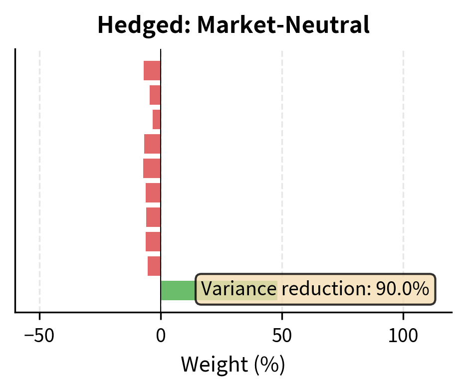
The decomposition shows that most portfolio variance comes from exposure to the first few principal components. For a market-neutral portfolio, we would want near-zero exposure to PC1 (the market factor).

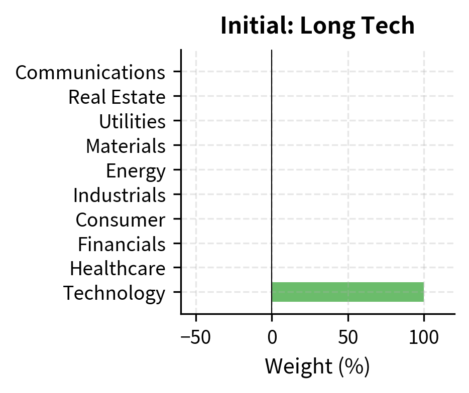
Constructing Factor-Hedged Portfolios
Understanding principal component exposures allows us to construct portfolios with specific factor characteristics:
By hedging out exposure to the first principal component, we significantly reduce portfolio variance. The hedged portfolio's performance will depend more on sector-specific factors (Technology's outperformance of other sectors) rather than overall market movements.
Limitations and Practical Considerations
While PCA is a powerful technique, several limitations affect its application to financial data.
Stationarity Assumptions
PCA assumes that the covariance structure is stable over time. In financial markets, this assumption often fails. Correlations spike during crises, factor loadings drift, and new factors emerge. The principal components extracted from 2005-2007 data looked very different from those needed to explain 2008 crisis dynamics. We address this by using rolling windows for PCA, but this introduces a tradeoff between stability (longer windows) and adaptability (shorter windows).
The yield curve factor structure is relatively stable because it reflects fundamental relationships between maturities. Equity factor structures are more volatile, especially for style factors like momentum or value, which experience periodic reversals in their relationship to underlying assets.
Interpretation Challenges
Unlike economic factors (market, size, value), statistical factors from PCA may lack clear interpretation. The second or third principal component of equity returns might capture a blend of industry effects, regional exposures, and macroeconomic sensitivities that resists simple characterization. This makes it difficult to communicate factor exposures to portfolio managers or clients who think in terms of economic factors.
Furthermore, PCA provides loadings that are only identified up to sign and rotation. The sign of each eigenvector is arbitrary (both and are valid eigenvectors), and when eigenvalues are close, the corresponding eigenvectors may mix across different samples.
Sample Size Requirements
Accurate estimation of covariance matrices requires observations substantially exceeding the number of variables. The rule of thumb suggests at least 3-5 observations per variable for stable eigenvalue estimates. With 500 stocks and daily data, this requires multiple years of history. For monthly data, the requirements become impractical.
This limitation is particularly severe in the tails of the eigenvalue distribution. The smallest eigenvalues are most prone to estimation error, often being indistinguishable from zero due to noise. Sophisticated techniques like random matrix theory help distinguish signal from noise in the eigenvalue spectrum, but these go beyond standard PCA.
The Factor Zoo Problem
In equity markets, academic research has identified hundreds of factors that predict returns. PCA offers no guidance on which statistical factors correspond to compensated risk factors versus data-mined anomalies. A factor that explains significant variance may offer no expected return premium. Conversely, important economic factors may explain little contemporaneous variance but matter greatly for expected returns. This distinction between risk factors (explaining variance) and priced factors (carrying risk premia) is fundamental but beyond PCA's scope.
Summary
This chapter developed Principal Component Analysis as a technique for extracting dominant factors from high-dimensional financial data. The key concepts include:
Mathematical foundation: PCA finds orthogonal directions of maximum variance through eigendecomposition of the covariance matrix. The eigenvalues quantify variance explained; the eigenvectors define the principal components.
Yield curve applications: The term structure of interest rates has remarkably low dimensionality. Three components (level, slope, and curvature) explain over 99% of yield curve movements. This finding simplifies risk management and enables efficient hedging with a small number of instruments.
Equity applications: Stock returns exhibit a factor structure dominated by market exposure, with additional components capturing sector, style, and other systematic effects. However, variance is less concentrated than in yield curves, and factor interpretations are less stable.
Risk management: PCA enables decomposition of portfolio variance by factor, identification of dominant risk sources, and construction of hedged portfolios with targeted factor exposures. Factor-based covariance matrices provide more stable inputs for portfolio optimization.
Connection to factor models: PCA extracts statistical factors that are optimal for variance explanation but may differ from economic factors used in asset pricing models. The relationship between statistical and economic factors is a theme we'll explore further when studying multi-factor models in Part IV.
The techniques from this chapter prepare you for the calibration and parameter estimation methods in the next chapter, where fitting models to market data relies heavily on similar linear algebra concepts.
Quiz
Ready to test your understanding? Take this quick quiz to reinforce what you've learned about Principal Component Analysis and Factor Extraction.

Comments