GARCH Volatility Models: Capturing Time-Varying Market Risk

In our study of the stylized facts of financial returns (Part III, Chapter 1), we observed a striking phenomenon. Large price movements tend to cluster together, followed by periods of relative calm. This volatility clustering violates the constant volatility assumption in the Black-Scholes-Merton framework we developed in Chapters 5 through 8. When we examined implied volatility and the volatility smile, we found that markets reject constant volatility, pricing options at different implied volatilities across strikes and maturities.

This chapter addresses a fundamental question: how do we model volatility that changes over time? The answer came from Robert Engle's groundbreaking ARCH model in 1982, which earned him the Nobel Prize in Economics. Tim Bollerslev extended this work with GARCH in 1986, creating what became the most widely used volatility model in finance. These models capture the empirical reality that today's volatility depends on yesterday's shocks and yesterday's volatility, creating the persistence and clustering we observe in markets.

Understanding time-varying volatility has profound implications. You need accurate volatility forecasts for Value at Risk calculations, exploit the gap between implied and forecasted volatility, and adjust position sizes based on volatility regimes. By the end of this chapter, you will be able to specify, estimate, and use GARCH models to capture the dynamic nature of financial volatility.

Recall from our time-series chapter that when we fit ARMA models to returns, we implicitly assumed that the error terms have constant variance. This property is called homoskedasticity, a term derived from the Greek words meaning "same dispersion." The assumption seems reasonable initially. If markets are efficient and information arrives randomly, why should the magnitude of price fluctuations vary systematically over time? Yet empirical observation tells a different story. Volatility itself becomes a dynamic, predictable quantity.

Mathematically, if we model returns as:

where:

• $r_t$: return at time $t$
• $\mu$: constant mean return
• $\epsilon_t$: residual or shock at time $t$

homoskedasticity requires:

where:

• $\text{Var}(\epsilon_t)$: variance of the error term
• $\sigma^2$: constant variance parameter

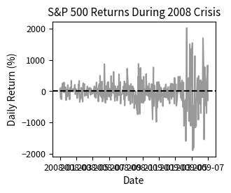
To appreciate what this assumption demands, consider what it implies. The variance of today's return shock must equal the variance of yesterday's shock, last month's shock, and the shock during the 2008 financial crisis. A single number, $\sigma^2$, must describe the dispersion of returns across all market conditions. This assumption is convenient for mathematical tractability, but it rarely holds for financial data. Let's see why by examining actual market data.

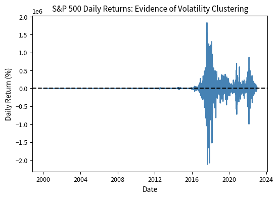
The visual evidence is compelling and immediate: returns during 2008-2009 swing wildly between large positive and negative values, creating a dense band of extreme observations that dominates that section of the chart. The COVID-induced volatility in early 2020 shows a similar pattern, with daily moves that would be extraordinary during normal times occurring repeatedly over several weeks. In contrast, periods like 2017 or 2013 exhibit remarkably calm, small daily movements, with the return series appearing almost compressed near the zero line. This is volatility clustering in action: large returns (of either sign) tend to be followed by large returns, and small returns tend to be followed by small returns. The phenomenon is so visually striking that no statistical test seems necessary, yet formal verification strengthens our confidence and quantifies the effect.

We can formally test for time-varying variance using several approaches, each building on the fundamental insight that if variance were truly constant, certain statistical patterns should be absent from the data. The simplest and most intuitive approach is to examine the autocorrelation of squared returns. The logic is simple. If volatility were constant, knowing that yesterday's squared return was large would tell you nothing about today's squared return; they would be independent and show zero autocorrelation. However, if volatility clusters, a large squared return yesterday signals we are in a high-volatility regime, making a large squared return today more likely. This creates positive autocorrelation in the squared return series.

In practice, squared returns show strong positive autocorrelation that persists for many lags. We verify this using the Ljung-Box test on squared returns, specifically checking the test statistic and p-value at 10 lags. This test aggregates autocorrelation evidence across multiple lags into a single statistic, making it a powerful diagnostic for detecting the type of serial dependence that violates homoskedasticity.

The highly significant Ljung-Box test confirms what we saw visually: squared returns are autocorrelated, meaning volatility exhibits persistence. The extremely small p-value allows us to reject the null hypothesis of no autocorrelation with overwhelming confidence. This finding is not unique to the S&P 500 or to our particular sample period; it emerges consistently across different markets, time periods, and asset classes. This is the phenomenon ARCH and GARCH models are designed to capture, and the universality of the finding motivates the development of a general modeling framework.

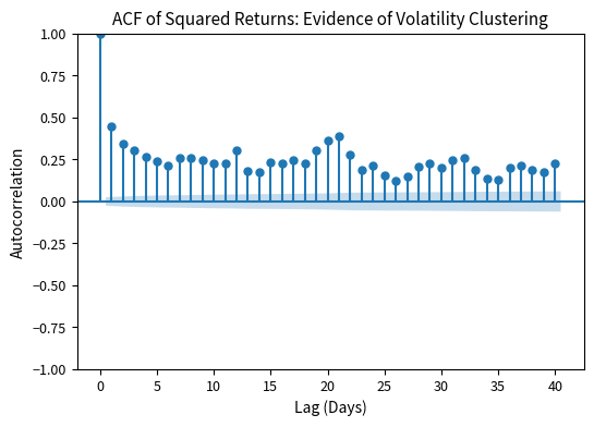
The ACF plot provides visual confirmation of what the Ljung-Box test detected statistically. The significant positive autocorrelation persists for many lags, with bars extending well beyond the confidence bands even at lags of 20 or 30 days. This slow decay indicates that volatility shocks have long-lasting effects, a key feature that GARCH models are designed to capture.

Robert Engle introduced the ARCH (Autoregressive Conditional Heteroskedasticity) model in 1982 to capture the observation that large shocks tend to be followed by large shocks. The name itself encodes the model's key features. "Autoregressive" indicates that the model uses its own past values to predict future values, much like the AR models we studied for returns themselves. "Conditional" emphasizes that we are modeling the variance conditional on past information, distinguishing it from the unconditional variance that averages across all market conditions. "Heteroskedasticity" simply means non-constant variance, the very phenomenon we seek to capture.

The key insight underlying ARCH is elegantly simple. Rather than treating variance as a fixed parameter to be estimated once from historical data, we model the conditional variance as a function of past squared residuals. This means that after observing a large price shock, our estimate of tomorrow's variance increases. Conversely, after a string of small price movements, we expect tomorrow's variance to be low. The model thus learns from recent market behavior and adapts its volatility estimate accordingly.

The ARCH(q) model specifies:

where:

• $r_t$: return at time $t$
• $\mu$: mean return
• $\epsilon_t$: innovation (shock) term

where the error term has time-varying variance:

where:

• $\sigma_t$: conditional standard deviation (volatility) at time $t$
• $z_t$: standardized residual, independent and identically distributed (i.i.d.)

This decomposition of the error term is crucial for understanding how ARCH works. The standardized residual $z_t$ captures the direction and magnitude of the shock in normalized terms, while $\sigma_t$ scales this shock to the appropriate level given current market conditions. When volatility is high, a typical standardized shock (say, $z_t = 1$) produces a large observed return shock $\epsilon_t$. The standardized residuals themselves are assumed to be i.i.d., meaning all the time-varying dynamics in returns come through the conditional variance.

The conditional variance follows:

where:

• $\sigma_t^2$: conditional variance at time $t$, given information at $t-1$
• $\omega$: constant term (intercept), must be positive
• $\alpha_i$: ARCH coefficients measuring the impact of past shocks
• $\epsilon_{t-i}^2$: squared residuals from $i$ periods ago (volatility shocks)
• $q$: number of lags in the ARCH model

This equation is the heart of the ARCH model. Reading it from right to left, today's conditional variance starts with a baseline level $\omega$ and then adds contributions from each of the past $q$ squared residuals. Each squared residual is weighted by its corresponding $\alpha_i$ coefficient, which measures how strongly that lag affects current variance. The summation structure creates the autoregressive nature: current variance depends on past squared shocks, just as AR models for returns make current returns depend on past returns.

The model captures a simple but powerful idea. If yesterday's return was unexpectedly large (positive or negative), today's conditional variance should be higher. Think of it as the market "remembering" recent turbulence. After a large price move, uncertainty increases, leading to more cautious or more reactive trading and larger subsequent price movements. The squaring of $\epsilon_{t-i}$ ensures that both positive and negative shocks increase volatility, consistent with the symmetric response we often observe in practice. A three percent gain creates as much "news" as a three percent loss in terms of its impact on expected future variance.

For the model to be well-defined and produce sensible variance forecasts, we need parameter constraints:

• $\omega > 0$ (positive baseline variance)
• $\alpha_i \geq 0$ for all $i$ (non-negative impact of shocks)
• $\sum_{i=1}^{q} \alpha_i < 1$ (ensures stationarity)

The first constraint guarantees that even in the complete absence of shocks, the model produces a positive variance. This makes economic sense: there is always some baseline uncertainty in financial markets. The second constraint ensures that past shocks cannot reduce variance, which would be counterintuitive. The third constraint, the stationarity condition, is particularly important because it guarantees that volatility doesn't explode over time. If the sum of the alpha coefficients exceeded one, a large shock would create even larger expected variance tomorrow, which would grow without bound.

When the stationarity condition holds, we find the unconditional (long-run) variance $\sigma^2$ by taking the expectation of the variance equation:

Solving for $\sigma^2$:

where:

• $\sigma^2$: unconditional (long-run) variance
• $\omega$: constant baseline variance parameter
• $\alpha_i$: ARCH coefficients summing to less than 1

This formula reveals that the unconditional variance depends on both the baseline parameter $\omega$ and the persistence of the process captured by the sum of the alpha coefficients. When this sum is close to one, the denominator becomes small, making the unconditional variance large. Intuitively, high persistence means that shocks have lasting effects on variance, inflating the long-run average level.

While ARCH captures volatility clustering, it has practical limitations that became apparent as researchers applied it to financial data:

• Many parameters needed: Capturing persistence in volatility often requires high-order ARCH models (large q), meaning many parameters to estimate.
• Slow decay: Volatility shocks persist for months empirically.
• No leverage effect: The symmetric treatment of positive and negative shocks misses that negative returns often increase volatility more than positive returns of equal magnitude.

If volatility shocks truly persist for, say, 60 trading days, we would need an ARCH(60) model with 61 parameters in the variance equation alone. Estimating so many parameters reliably requires enormous datasets and provides little insight into the underlying dynamics. This parameter proliferation problem motivated the development of GARCH, which achieves the same modeling power with remarkable parsimony.

Tim Bollerslev's 1986 GARCH (Generalized ARCH) model elegantly addresses ARCH's limitations by adding lagged conditional variance terms. This simple addition has major implications. Instead of requiring many lagged squared residuals to capture persistence, GARCH introduces a feedback mechanism: yesterday's conditional variance directly affects today's conditional variance. With this addition, GARCH(1,1) often fits as well as or better than high-order ARCH models with far fewer parameters.

The intuition behind adding lagged variance terms is that conditional variance itself carries information about the volatility state. If yesterday's conditional variance was high, we were in a turbulent market environment. That turbulence is likely to continue regardless of whether yesterday's specific realized shock was large or small. The lagged variance term captures this "regime" information that squared residuals alone might miss.

The GARCH(p,q) model specifies:

where:

• $\sigma_t^2$: conditional variance at time $t$
• $\omega$: constant parameter
• $\alpha_i$: ARCH coefficients measuring impact of past shocks
• $\epsilon_{t-i}^2$: squared residuals from $i$ periods ago
• $\beta_j$: GARCH coefficients measuring the impact of past variance
• $\sigma_{t-j}^2$: lagged conditional variance terms
• $p$: number of GARCH lags
• $q$: number of ARCH lags

The addition of $\beta_j \sigma_{t-j}^2$ terms creates a feedback mechanism: high variance yesterday directly contributes to high variance today, beyond just the impact of past shocks. This means that even if yesterday's specific return was modest, if we were in a high-variance state, that elevated variance carries forward into today's forecast. The GARCH terms essentially summarize the effect of all historical shocks, weighted by their distance from the present.

The GARCH(1,1) specification is by far the most widely used variant in both academic research and industry practice:

where:

• $\sigma_t^2$: conditional variance for day $t$
• $\omega$: constant parameter
• $\alpha$: coefficient on the lagged squared residual (news impact)
• $\epsilon_{t-1}^2$: squared return shock from previous day
• $\beta$: coefficient on the lagged variance (persistence)
• $\sigma_{t-1}^2$: conditional variance from previous day

This equation admits a natural interpretation. Today's conditional variance consists of three components.

• Baseline level $\omega$: Represents the minimum variance floor
• News component $\alpha \epsilon_{t-1}^2$: Captures how yesterday's specific return shock affects the variance estimate. If yesterday's shock was large, this term increases today's variance.
• Memory component $\beta \sigma_{t-1}^2$: Carries forward yesterday's overall volatility state. If you were in a high-volatility regime yesterday, that regime persists to some degree today.

The parameter constraints for stationarity are.

• $\omega > 0$ (positive baseline variance) 0$,$\beta \geq 0$
• $\alpha + \beta < 1$

When these hold, we find the unconditional variance by setting expectations $E[\sigma_t^2] = E[\epsilon_{t-1}^2] = \bar{\sigma}^2$ in the GARCH equation:

Thus:

where:

• $\bar{\sigma}^2$: long-run unconditional variance
• $\omega$: constant parameter
• $\alpha, \beta$: ARCH and GARCH coefficients
• $\alpha + \beta$: persistence of the process (must be $< 1$)

This result shows that the unconditional variance depends inversely on the quantity $(1 - \alpha - \beta)$. When $\alpha + \beta$ is close to one, the denominator approaches zero and the unconditional variance becomes very large. This makes sense: high persistence means shocks have lasting effects, inflating the average variance level over time.

The sum $\alpha + \beta$ measures volatility persistence. This quantity determines how quickly volatility reverts to its long-run mean after a shock. Higher values mean slower reversion, with volatility remaining elevated (or depressed) for longer periods following a disturbance.

To see this mathematically, we can rewrite GARCH(1,1) in terms of deviations from unconditional variance. After a shock at time $t$, the expected conditional variance at time $t+h$ is:

where:

• $E[\sigma_{t+h}^2 | \mathcal{F}_t]$: expected conditional variance at time $t+h$ given information at time $t$
• $\bar{\sigma}^2$: unconditional long-run variance
• $\alpha + \beta$: persistence parameter (decay rate)
• $h$: forecast horizon (days ahead)
• $\sigma_t^2$: current conditional variance

This formula has a powerful interpretation. The deviation of conditional variance from its long-run mean decays exponentially at rate $\alpha + \beta$. If today's variance is above average, the expected variance tomorrow will be closer to average, but not all the way there. The gap shrinks by a factor of $(\alpha + \beta)$ each day. When persistence is high (say, 0.98), only 2% of the gap closes each day, meaning elevated volatility persists for many weeks.

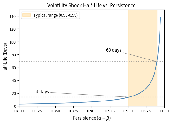
We define the half-life $k$ as the time required for the shock's impact to reduce by 50%:

Therefore:

where:

• $\text{Half-life}$: time required for a shock's impact to reduce by 50%
• $\alpha + \beta$: persistence parameter

In financial data, $\alpha + \beta$ typically ranges from 0.95 to 0.99, implying half-lives of 14 to 69 days. Volatility shocks are highly persistent, meaning that after a crisis or turbulent period, markets do not quickly return to normal. Instead, elevated volatility fades gradually over weeks and months, a pattern that has important implications for risk management and option pricing.

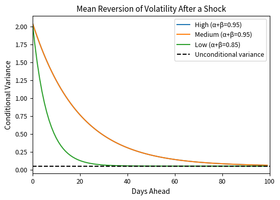
This figure illustrates the key insight: volatility mean-reverts, but slowly. After a large shock that elevates variance above its long-run level, it takes many days for conditional variance to return to its equilibrium. The decay is exponential, with higher persistence parameters producing slower convergence. This persistence is what makes GARCH models so useful for forecasting: we can predict that elevated volatility will gradually decline, and depressed volatility will gradually rise, toward the long-run average.

There is an elegant connection between GARCH and ARMA models that illuminates why GARCH(1,1) is so parsimonious. Just as ARMA models capture the autocorrelation structure of returns, GARCH can be viewed as an ARMA model for the variance process. This connection not only provides theoretical insight but also justifies why a single GARCH lag often suffices.

Define the variance innovation as:

where:

• $v_t$: variance innovation (martingale difference sequence)
• $\epsilon_t^2$: realized squared return (proxy for volatility)
• $\sigma_t^2$: conditional variance (expected volatility)

This represents the difference between the realized squared return and its conditional expectation (the variance). The variance innovation $v_t$ is a martingale difference sequence. This means it has zero expected value and is unpredictable from past information. It captures the surprise in realized variance relative to what the model predicted.

We substitute $\sigma_t^2 = \epsilon_t^2 - v_t$ into the GARCH(1,1) equation. Similarly substituting for $t-1$, we derive the ARMA structure:

where:

• $\epsilon_t^2$: squared return at time $t$
• $\omega, \alpha, \beta$: GARCH parameters
• $v_t$: variance innovation term

This is an ARMA(1,1) model for squared returns! The AR coefficient is $(\alpha + \beta)$ and the MA coefficient is $-\beta$. The connection explains why GARCH(1,1) is so parsimonious: it captures the same dynamics as an ARMA(1,1) for the variance process. Just as ARMA(1,1) often suffices for modeling the autocorrelation structure of returns, GARCH(1,1) suffices for modeling the autocorrelation structure of squared returns. The elegance of this representation also facilitates theoretical analysis of GARCH properties.

In our study of stylized facts, we noted that negative returns tend to increase volatility more than positive returns of the same magnitude. This asymmetry, called the leverage effect, has a financial explanation. When stock prices fall, firms become more leveraged (debt-to-equity ratio rises), increasing the riskiness of equity. A firm with fixed debt obligations becomes more precarious as its equity value declines, making future returns more uncertain.

Beyond the mechanical leverage explanation, psychological and behavioral factors may contribute. Negative returns may trigger fear and uncertainty among investors, leading to more volatile trading behavior. Margin calls during market declines force liquidations that amplify price movements. Whatever the cause, the empirical regularity is robust: bad news moves volatility more than good news.

Standard GARCH treats positive and negative shocks symmetrically through the $\epsilon_{t-1}^2$ term, so a positive two percent return and a negative two percent return contribute equally to tomorrow's variance. Several extensions address this limitation by allowing the model to distinguish between good and bad news.

Nelson's 1991 EGARCH model specifies the log of conditional variance:

where:

• $\ln(\sigma_t^2)$: natural log of conditional variance
• $\omega$: constant parameter
• $\frac{\epsilon_{t-1}}{\sigma_{t-1}}$: standardized residual $z_{t-1}$
• $\alpha$: coefficient on the magnitude of the shock (symmetric effect)
• $\gamma$: coefficient on the sign of the shock (asymmetric/leverage effect)
• $E\left| \frac{\epsilon_{t-1}}{\sigma_{t-1}} \right|$: expected absolute value of standardized residual
• $\beta$: persistence coefficient

The key features of EGARCH distinguish it from other asymmetric specifications:

• Log specification: Modeling the log of variance rather than variance itself ensures $\sigma_t^2 > 0$ without requiring parameter constraints. The exponential function always produces positive variance.
• Standardized residuals: Uses $z_{t-1} = \epsilon_{t-1}/\sigma_{t-1}$ for stability. Dividing by the conditional standard deviation normalizes the shock, making coefficients more interpretable and comparable across different volatility levels.
• Asymmetry parameter $\gamma$: Negative $\gamma$ captures the leverage effect, where negative shocks increase volatility more than positive shocks. negative standardized residual adds to log variance both through the magnitude term (which responds to the absolute value) and directly through the sign term (which is now positive when $z_{t-1}$ is negative).

Glosten, Jagannathan, and Runkle (1993) proposed a simpler asymmetric specification that modifies standard GARCH in a more intuitive way:

where $I_{t-1}$ is an indicator function:

where:

• $\sigma_t^2$: conditional variance
• $\omega$: constant parameter
• $\alpha$: coefficient on symmetric response
• $\gamma$: coefficient on asymmetric leverage effect
• $I_{t-1}$: binary indicator for negative shocks
• $\epsilon_{t-1}$: past return shock
• $\beta$: coefficient on past variance
• $\sigma_{t-1}^2$: lagged conditional variance

The interpretation is straightforward, requiring no logarithms or standardization.

• Positive shocks contribute $\alpha \epsilon_{t-1}^2$ to variance
• Negative shocks contribute $(\alpha + \gamma) \epsilon_{t-1}^2$ to variance
• $\gamma > 0$ implies negative shocks have a larger impact (leverage effect)

The indicator function acts as a switch. It turns on the additional $\gamma \epsilon_{t-1}^2$ term only when the previous shock was negative. This creates a piecewise linear response to shocks, with a steeper slope for negative shocks than for positive ones. The simplicity of this specification makes it easy to interpret and estimate, contributing to its popularity in applied work.

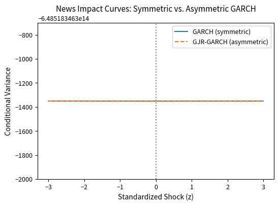
The news impact curve reveals the key difference between symmetric and asymmetric models. Under standard GARCH, the curve is a parabola centered at zero: positive and negative shocks of equal magnitude have identical effects on variance. Under GJR-GARCH, the variance response is steeper for negative shocks, creating an asymmetric parabola with a kink at zero. A negative two standard deviation shock increases variance more than a positive two standard deviation shock, consistent with empirical observations in equity markets. This visual representation makes clear exactly what the asymmetry parameter captures.

GARCH parameters are typically estimated via Maximum Likelihood Estimation (MLE). As discussed in the statistical inference chapter (Part I, Chapter 4), MLE finds parameters that maximize the probability of observing the data. For GARCH models, this means finding the variance equation parameters that make our observed return sequence most probable.

The likelihood function for GARCH builds on the assumption that standardized residuals are i.i.d. with a known distribution. Given parameters, we can compute the conditional variance at each point in time. We then evaluate how likely each observed return is given that conditional variance. Returns that are small relative to their conditional variance contribute more to the likelihood; returns that are large relative to their variance are penalized.

For a sample of returns $\{r_1, r_2, \ldots, r_T\}$, assuming conditional normality, the log-likelihood is:

where:

• $\mathcal{L}(\theta)$: log-likelihood of the sample
• $\ln(\sigma_t^2)$: penalty term for higher variance (uncertainty)
• $\frac{(r_t - \mu)^2}{\sigma_t^2}$: penalty term for poor fit (squared standardized residual)
• $\theta$: vector of parameters $(\mu, \omega, \alpha, \beta)$
• $T$: sample size
• $\sigma_t^2$: conditional variance at time $t$
• $r_t$: return at time $t$

This expression has an intuitive structure. The first term inside the brackets is a constant that normalizes the density. The second term $\ln(\sigma_t^2)$ penalizes high variance. All else equal, the model prefers parameters that produce lower variance because this implies more precision in the forecasts. The third term $(r_t - \mu)^2 / \sigma_t^2$ penalizes returns that are large relative to the predicted variance. The model prefers parameters that make large returns occur when variance is high and small returns occur when variance is low.

The estimation proceeds as follows:

1. Initialize: Set starting values for parameters and initial variance (often the sample variance)
2. Recursion: For each $t$, compute $\sigma_t^2$ using the GARCH equation
3. Evaluate: Calculate the log-likelihood contribution from each observation
4. Optimize: Use numerical optimization to find parameters maximizing total log-likelihood

The recursive structure of GARCH means that the conditional variance at time $t$ depends on the conditional variance at time $t-1$. We must specify an initial variance to start the recursion, typically set to the unconditional variance implied by preliminary parameter estimates or simply the sample variance. As the sample grows, the influence of this initialization diminishes, but for short samples it can matter.

While conditional normality is convenient, you know from our stylized facts chapter that return distributions have fatter tails than normal. Even after accounting for time-varying variance, standardized residuals often exhibit excess kurtosis. This suggests that the normal distribution may not adequately capture the probability of extreme returns. Two common alternatives address this limitation:

• Student-t distribution: Adds a degrees-of-freedom parameter $\nu$ to capture excess kurtosis, where lower $\nu$ means fatter tails. As $\nu$ approaches infinity, the Student-t converges to the normal distribution. Typical estimates for financial data fall between 4 and 10, indicating substantial tail risk.
• Generalized Error Distribution (GED): Flexible family that nests the normal as a special case. A shape parameter controls the tail thickness, with values less than 2 producing fatter tails than normal and values greater than 2 producing thinner tails.

Using fat-tailed distributions often improves model fit and produces more accurate tail risk estimates. For risk management applications where extreme events matter most, the choice of error distribution can substantially affect VaR and expected shortfall calculations.

Let's estimate a GARCH(1,1) model on S&P 500 returns. We use the arch_model function with vol='GARCH', p=1, and q=1 to specify the GARCH(1,1) structure, and set dist='t' to use Student-t distributed errors, which account for the fat tails observed in financial data.

The results reveal key features of S&P 500 volatility:

• High persistence: The sum $\alpha + \beta$ is very close to 1, indicating that volatility shocks decay slowly, which explains why elevated volatility during crises persists for months. A half-life of several weeks means that market turbulence does not quickly dissipate.
• Low $\alpha$, high $\beta$: Most of today's variance comes from yesterday's variance level, with only a small fraction attributable to yesterday's shock. This suggests smooth, persistent volatility dynamics rather than erratic jumps. The dominance of the beta term means volatility evolves gradually, with each day's level heavily influenced by the recent past.
• Fat tails: The Student-t degrees of freedom around 5 to 8 confirms significant excess kurtosis in the standardized residuals, even after accounting for time-varying volatility. The data still produce more extreme observations than a normal distribution would predict, which motivates using heavy-tailed error distributions.

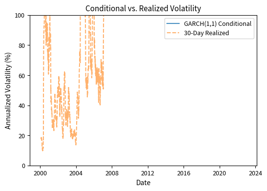
The GARCH conditional volatility reacts immediately to new return observations, while the rolling realized volatility lags because it weights all observations in the window equally. During the 2008 crisis and 2020 COVID shock, GARCH captures the volatility spike almost instantaneously, whereas rolling measures take weeks to fully adjust. This responsiveness makes GARCH particularly valuable for risk management during turbulent periods when accurate, timely volatility estimates matter most.

Let's compare symmetric GARCH with asymmetric GJR-GARCH to test for leverage effects. By setting o=1 in the arch_model function, we enable the asymmetric term that captures the different impacts of positive and negative shocks. This comparison allows us to assess whether the additional complexity of asymmetry is warranted by the data.

The significantly positive asymmetry parameter confirms the leverage effect: negative returns increase volatility more than positive returns. The magnitude of $\gamma$ indicates that the effect is economically meaningful, not just statistically significant. The lower AIC and BIC for GJR-GARCH indicate better fit despite the additional parameter, suggesting the asymmetry is economically meaningful and worth including in the model.

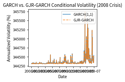
The comparison during the 2008 crisis period reveals how the asymmetric GJR-GARCH model responds more strongly to negative shocks. Following the large negative returns in September-October 2008, GJR-GARCH produces higher volatility estimates than the symmetric GARCH model. This difference reflects the leverage effect: the asymmetric model correctly assigns greater volatility impact to the severe market declines during the crisis.

A well-specified GARCH model should produce standardized residuals that are approximately i.i.d. with no remaining autocorrelation in their squared values. If the model has successfully captured the volatility dynamics, the standardized residuals should look like random noise, exhibiting none of the clustering patterns we observed in the raw returns.

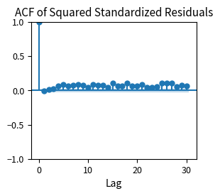
The much higher p-value for the Ljung-Box test on standardized squared residuals (compared to raw squared returns) indicates the GARCH model successfully captures most of the volatility clustering. The raw squared returns showed overwhelming evidence of autocorrelation, while the standardized squared residuals show much weaker dependence. The ACF plot shows minimal remaining autocorrelation, confirming that the model adequately describes the variance dynamics. While no model is perfect, these diagnostics suggest GARCH(1,1) provides a reasonable description of the volatility process.

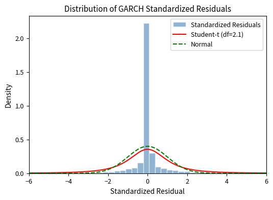
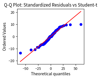
The histogram confirms that the Student-t distribution provides a better fit than the normal distribution for the standardized residuals. The observed distribution has heavier tails than normal, with more extreme observations in both directions than a Gaussian would predict. The fitted Student-t distribution with the estimated degrees of freedom captures this excess kurtosis, validating our choice of error distribution and explaining why risk measures based on normal assumptions would underestimate tail risk.

• ω (omega): Constant baseline variance term, must be positive
• α (alpha): ARCH parameter measuring impact of past squared shocks (news), with higher values indicating more sensitivity to recent events
• β (beta): GARCH parameter measuring persistence of past variance, with higher values meaning volatility clusters last longer
• γ (gamma): Asymmetry parameter (in GJR-GARCH), where positive values indicate negative shocks increase volatility more than positive shocks
• ν (nu): Degrees of freedom for the Student-t distribution, with lower values indicating fatter tails and higher probability of extreme events
• α + β: Persistence measure, with values close to 1 indicating volatility shocks decay very slowly

The primary application of GARCH models is forecasting future volatility. For GARCH(1,1), the one-step-ahead forecast is straightforward:

where:

• $\hat{\sigma}_{t+1}^2$: forecasted variance for the next period
• $\omega, \alpha, \beta$: estimated model parameters
• $\epsilon_t^2$: today's squared return shock
• $\sigma_t^2$: today's conditional variance

Given today's shock $\epsilon_t$ and variance $\sigma_t^2$, tomorrow's variance forecast is simply the GARCH equation evaluated at current values. This forecast incorporates two sources of information: the specific return shock that just occurred and the overall volatility state. The simplicity of this calculation makes GARCH particularly attractive for real-time applications where you must update forecasts daily.

For longer horizons, you iterate the GARCH equation forward. Since the expected squared shock equals the variance ($E_T[\epsilon_{T+k}^2] = E_T[\sigma_{T+k}^2]$), the forecast follows a recursive pattern:

where:

• $E_T[\sigma_{T+k}^2]$: expected variance $k$ steps ahead
• $\omega, \alpha, \beta$: model parameters
• $E_T[\sigma_{T+k-1}^2]$: expected variance at the previous step

Subtracting the unconditional variance $\bar{\sigma}^2$ from both sides reveals the mean-reverting dynamic:

where:

• $E_T[\sigma_{T+k}^2] - \bar{\sigma}^2$: expected deviation of variance from the long-run average at horizon $k$
• $\alpha + \beta$: persistence parameter determining decay rate
• $E_T[\sigma_{T+k-1}^2] - \bar{\sigma}^2$: expected deviation at the previous step

This relationship shows that the expected deviation from unconditional variance shrinks by a factor of $(\alpha + \beta)$ each period. Starting from any initial variance, forecasts converge geometrically toward the long-run level. Iterating this relationship $h-1$ times yields the $h$-step-ahead forecast from time $T$:

where:

• $E_T[\sigma_{T+h}^2]$: expected variance $h$ days ahead given info at $T$
• $\bar{\sigma}^2$: unconditional long-run variance
• $\alpha, \beta$: persistence parameters
• $h$: forecast horizon
• $\hat{\sigma}_{T+1}^2$: next day's variance forecast

As the horizon $h$ increases, the forecast converges to the unconditional variance. This is mean reversion in action. As you become increasingly uncertain about future volatility, your best guess converges to the long-run average. At very long horizons, your specific knowledge of current market conditions becomes irrelevant, and you fall back on the unconditional variance as your forecast.

The volatility term structure shows how GARCH forecasts evolve with horizon. If current volatility is above the long-run level, the forecast gradually declines; if below, it gradually rises. This mean-reverting behavior is economically sensible and distinguishes GARCH from naive historical measures that assume volatility is constant. The shaded region illustrates the increasing uncertainty associated with longer forecast horizons. Traders and risk managers can use this term structure to set appropriate volatility assumptions for options and risk calculations at different maturities.

You use GARCH to estimate time-varying Value at Risk. Rather than assuming constant volatility, you update daily VaR with the conditional variance:

where:

• $\text{VaR}_{t,\alpha}$: Value at Risk at confidence level $\alpha$ for time $t$
• $\mu$: expected daily return
• $z_\alpha$: lower tail quantile of the distribution (typically negative)
• $\sigma_t$: conditional volatility forecast

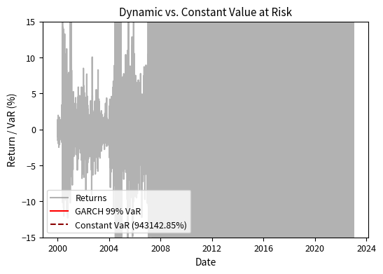
The dynamic VaR adapts to market conditions. During the 2008 crisis, GARCH VaR increases to reflect elevated risk, then gradually declines as markets stabilize. By contrast, constant VaR underestimates risk during crises and overestimates during calm periods. This adaptive property makes GARCH invaluable for risk management.

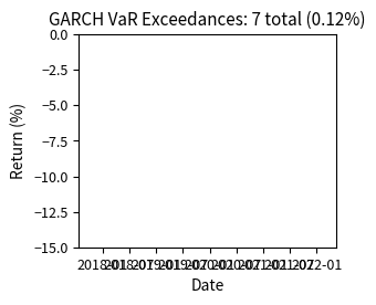
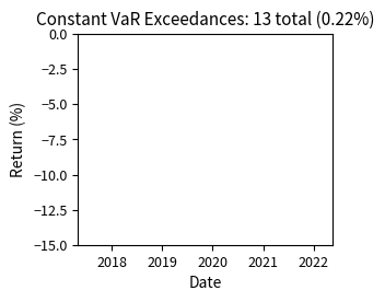
The exceedance analysis reveals a critical difference between the two approaches. The constant VaR produces clustered violations during the 2008 and 2020 crisis periods, when the fixed threshold was inadequate for the elevated volatility. The GARCH-based VaR distributes exceedances more uniformly across time because it adapts to changing market conditions. For a 99% VaR, we expect approximately 1% of observations to exceed the threshold; the dynamic approach comes closer to achieving this uniform coverage.

The Black-Scholes framework assumes constant volatility, but GARCH shows volatility is predictably time-varying. This has several implications for option pricing:

• Volatility term structure: GARCH implies that implied volatility should vary with option maturity, which is consistent with the term structure we observe in markets
• Volatility forecasting for trading: If GARCH forecasts volatility higher (lower) than current implied volatility, options may be underpriced (overpriced)
• GARCH option pricing models: Academic research has developed option pricing formulas under GARCH dynamics, though these are more complex than Black-Scholes

The connection between GARCH forecasts and implied volatility creates opportunities for volatility trading strategies. We'll explore regression-based approaches to this relationship in the next chapter.

GARCH volatility forecasts can inform portfolio allocation. A simple volatility timing strategy adjusts exposure based on predicted risk:

where:

• $w_t$: portfolio weight for the risky asset
• $\sigma_{\text{target}}$: target volatility level
• $\hat{\sigma}_{t+1}$: forecasted volatility for the next period

If predicted volatility is high, you reduce exposure to maintain constant risk. When low, you increase exposure. This approach connects to the portfolio optimization frameworks we'll develop in Part IV.

GARCH models successfully capture several stylized facts:

• Volatility clustering: The autoregressive structure ensures that large shocks lead to elevated variance
• Persistence: High $\alpha + \beta$ creates the slow decay observed in practice
• Fat tails: Even with normal errors, the mixture of variances produces unconditionally fat-tailed returns
• Leverage effects: Asymmetric variants like GJR-GARCH capture the negative correlation between returns and volatility

GARCH has important limitations, though:

• No jumps: GARCH assumes volatility evolves continuously. Major events like central bank announcements or geopolitical shocks can cause discrete volatility jumps that GARCH cannot capture.
• Univariate: GARCH doesn't naturally extend to capturing correlations across assets. Multivariate extensions (DCC-GARCH, BEKK) exist but come at the cost of substantial complexity.
• Returns-only information: GARCH models volatility based solely on past returns, ignoring other relevant information like option prices, macroeconomic indicators, or sentiment measures.
• Extreme tails: While GARCH captures unconditional fat tails through time-varying variance, it may not fully account for the extreme tails observed in practice, particularly during crisis periods.

Several practical issues arise when applying GARCH models. Model selection between GARCH, GJR-GARCH, EGARCH, and other variants requires judgment. Information criteria like AIC and BIC help, but out-of-sample forecast evaluation is the gold standard. The degrees-of-freedom parameter for Student-t errors and the lag orders (p, q) require careful selection.

Parameter stability is another concern. GARCH parameters estimated over one period may not remain stable, particularly across different volatility regimes. Rolling or expanding window estimation can reveal parameter drift. Very high persistence (near-integrated GARCH with α + β ≈ 1) can cause numerical issues and unrealistic long-run variance estimates.

For intraday applications, standard daily GARCH may be insufficient. High-frequency volatility modeling uses realized variance measures and represents an active research area.

Despite its limitations, GARCH transformed how practitioners and academics think about volatility. Before Engle's work, constant volatility was the default assumption. GARCH provided a tractable, estimable framework for time-varying volatility that:

• Improved risk measurement and capital allocation
• Enhanced derivative pricing and hedging
• Enabled volatility forecasting for trading strategies
• Established volatility itself as an object of study and trading

Robert Engle's 2003 Nobel Prize recognized these contributions. Today, GARCH and its variants remain the workhorses of volatility modeling, forming the foundation upon which more sophisticated approaches build.

This chapter developed the essential tools for modeling time-varying volatility in financial markets:

Core concepts:

• Volatility clusters because large shocks tend to be followed by large shocks, and small shocks by small shocks
• ARCH models capture this by making conditional variance depend on past squared returns
• GARCH adds lagged variance terms, achieving parsimony. GARCH(1,1) captures the same dynamics as high-order ARCH with just three parameters

Key relationships:

• The persistence $\alpha + \beta$ determines how quickly volatility reverts to its long-run mean
• Typical financial data shows persistence of 0.95 to 0.99, meaning volatility shocks decay slowly
• Asymmetric models like GJR-GARCH capture the leverage effect where negative returns increase volatility more than positive returns

Practical applications include:

• Parameter estimation via maximum likelihood, typically with Student-t errors to capture fat tails
• Model diagnostics through Ljung-Box tests on squared standardized residuals
• Volatility forecasting for risk management (dynamic VaR) and trading (volatility timing)

Limitations to remember:

• GARCH is univariate and ignores cross-asset dependencies
• Continuous volatility evolution misses discrete jumps
• Parameters may be unstable across different market regimes

The next chapter on regression analysis will extend our toolkit for understanding relationships in financial data, including how GARCH volatility forecasts relate to market-implied volatility and other explanatory variables.

Ready to test your understanding? Take this quick quiz to reinforce what you've learned about volatility modeling and GARCH.