

A comprehensive guide to spline regression covering B-splines, knot selection, natural cubic splines, and practical implementation. Learn how to model complex non-linear relationships with piecewise polynomials.

This article is part of the free-to-read Machine Learning from Scratch
Choose your expertise level to adjust how many terms are explained. Beginners see more tooltips, experts see fewer to maintain reading flow. Hover over underlined terms for instant definitions.
Spline Regression
Spline regression represents a sophisticated approach to modeling non-linear relationships that addresses many of the limitations inherent in polynomial regression. While polynomial regression fits a single high-degree polynomial across the entire range of data, spline regression divides the data into segments and fits separate, typically lower-degree polynomials to each segment. These segments are connected at specific points called knots, ensuring smooth transitions between adjacent polynomial pieces.
The fundamental insight behind spline regression is that complex non-linear relationships can often be better approximated by combining simpler, local polynomial functions rather than using a single, complex polynomial across the entire domain. This approach allows the model to capture local patterns and adapt to different regions of the data while maintaining mathematical tractability. Unlike polynomial regression, which can suffer from Runge's phenomenon (oscillations at the edges) and global overfitting, splines provide more stable and interpretable fits.
Spline regression distinguishes itself from other non-linear methods through its piecewise polynomial nature and the concept of continuity constraints. The most common types are cubic splines, which use cubic polynomials in each segment and ensure that the function, its first derivative, and second derivative are all continuous at the knot points. This creates smooth curves that can capture complex patterns while avoiding the erratic behavior often seen in high-degree polynomials. The method maintains the linear regression framework by treating the spline basis functions as features, making it computationally efficient and statistically interpretable.
Spline regression provides flexibility and control through the choice of knot number and placement, allowing us to balance model complexity with smoothness. The resulting models often provide better generalization than polynomial regression while remaining more interpretable than black-box methods like neural networks.
Advantages
Spline regression offers several compelling advantages that make it a powerful tool for non-linear modeling. First, it provides excellent local flexibility while maintaining global smoothness. Unlike polynomial regression, which applies the same functional form across the entire domain, splines can adapt to different regions of the data, capturing local patterns without being influenced by distant observations. This local adaptation makes splines particularly effective for data with varying curvature or multiple regimes.
Second, spline regression offers superior numerical stability compared to high-degree polynomial regression. By using lower-degree polynomials in each segment, we avoid the numerical issues that plague high-degree polynomials, such as ill-conditioned matrices and extreme sensitivity to small changes in the data. The piecewise approach also makes the method more robust to outliers, as the influence of an outlier is typically confined to its local segment rather than affecting the entire model.
Finally, splines provide excellent control over model complexity through the strategic placement of knots. We can increase the number of knots to capture more complex patterns or reduce them to enforce smoother fits. This control allows for a principled approach to the bias-variance trade-off, where we can tune the model's flexibility based on the amount of data available and the underlying complexity of the relationship we're trying to model.
Disadvantages
Despite its advantages, spline regression comes with several important limitations to consider. The most significant challenge is the selection of knot locations and the number of knots. Unlike polynomial regression, where we only need to choose the degree, spline regression requires us to make decisions about where to place the knots, which can significantly impact model performance. Poor knot placement can lead to overfitting in some regions while underfitting in others, and there's no universally optimal strategy for knot selection.
Another major concern is the computational complexity that increases with the number of knots. Each additional knot increases the number of parameters in the model, and the computational cost grows accordingly. For datasets with many observations and complex relationships requiring many knots, the computational burden can become substantial. Additionally, the method can suffer from overfitting when too many knots are used, especially with limited data, leading to poor generalization performance.
The interpretability of spline models can also be challenging, particularly when many knots are involved. While the piecewise polynomial nature provides some interpretability, understanding the overall relationship becomes more difficult as the number of segments increases. Unlike simple polynomial regression, where we can easily interpret the coefficients, spline coefficients represent local effects that must be considered in the context of the entire piecewise function.
The choice of knot locations is often more critical than the choice of polynomial degree in polynomial regression. Poor knot placement can lead to models that fit the training data well but generalize poorly, making cross-validation and careful model selection important for successful spline regression.
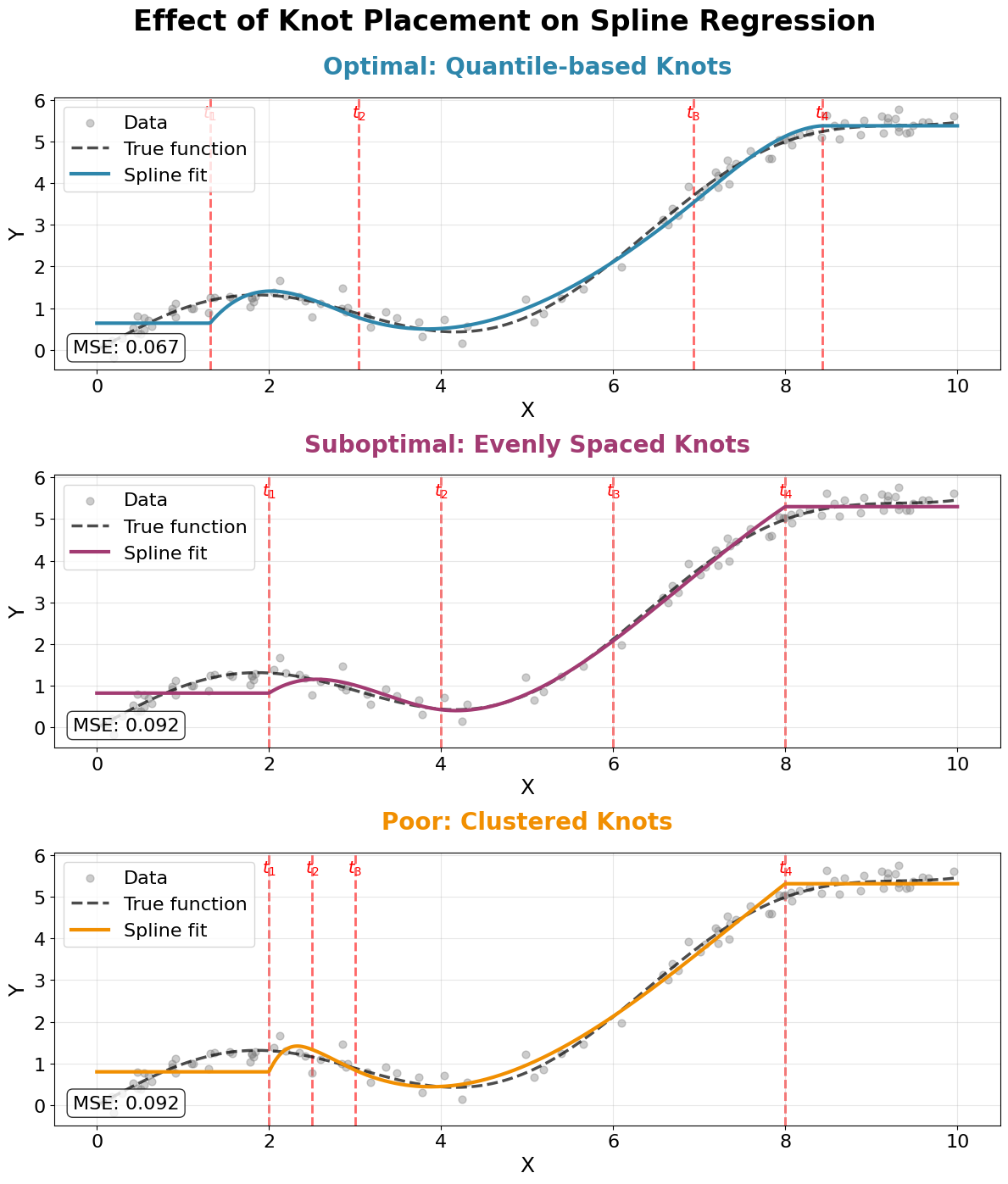
This visualization demonstrates why knot placement is critical for spline regression success. The optimal strategy places knots at data quantiles, ensuring adequate flexibility in regions with varying data density. Evenly spaced knots may work reasonably well but don't adapt to data distribution. Poorly placed knots (clustered in one region) lead to overfitting where knots are dense and underfitting where they're sparse, resulting in poor overall performance despite having the same number of knots as the optimal configuration.
Formula
The spline regression model extends linear regression by using piecewise polynomial basis functions instead of simple polynomial terms. We'll start with the most intuitive form and progressively build to the complete mathematical framework, explaining every piece of notation along the way.
Basic Spline Concept
Let's begin by understanding what a spline function actually is. A spline function is a special type of function that is constructed by joining together multiple polynomial pieces. Think of it like connecting different curved segments to create one smooth, continuous curve.
The mathematical definition of a spline function of degree with knots at positions is:
Let's break down every piece of this notation:
-
: This is our spline function. It takes an input value and returns a corresponding output value. The function is defined piecewise, meaning it has different formulas for different ranges of .
-
: This represents the degree of the spline. If , we have linear splines (straight line segments). If , we have quadratic splines (parabolic segments). If , we have cubic splines (cubic polynomial segments). Cubic splines are most commonly used because they provide a good balance between flexibility and smoothness.
-
: These are called knots or knot points. They are specific values of where we transition from one polynomial piece to another. Think of them as "break points" where the function changes its behavior. For example, if and , then:
- For all values less than or equal to 3, we use polynomial
- For all values between 3 and 7, we use polynomial
- For all values greater than 7, we use polynomial
-
: Each is a polynomial of degree or less. For example, if (cubic splines), then each might look like:
where are coefficients that we need to determine.
Interval Notation:
The notation , , and uses mathematical interval notation:
- : This means "all values of that are less than or equal to "
- : This means "all values of that are greater than AND less than or equal to "
- : This means "all values of that are greater than "
The key insight is that we're not fitting a single polynomial across the entire range, but rather different polynomials in different regions, connected at the knot points. This allows us to capture local patterns in the data while maintaining smoothness across the entire function.

This visualization demonstrates the fundamental concept of spline regression: instead of using a single complex polynomial across the entire range, we use simpler polynomials in different regions. Each colored segment represents a different cubic polynomial, and these pieces connect smoothly at the knots (red dashed lines). The complete spline function is the combination of all these pieces, creating a flexible curve that can adapt to local patterns in the data.
Cubic Spline Regression Model
The most common form is cubic spline regression, where we use cubic polynomials in each segment. The cubic spline regression model can be written as:
where:
- : the response variable (the value we want to predict)
- : the intercept term (baseline value when all basis functions are zero)
- : the coefficient for the -th B-spline basis function (weight assigned to basis function )
- : the -th B-spline basis function evaluated at input (building block of the spline)
- : the total number of B-spline basis functions (determined by the number of knots and degree)
- : the input variable or predictor
- : the error term (captures unexplained variation in the response)
The basis functions are constructed to ensure continuity and smoothness at the knot points.
B-spline Basis Functions
The most elegant way to construct spline basis functions is through B-splines (Basis splines). B-splines are special functions that serve as the "building blocks" for constructing any spline function. Think of them as standardized, reusable components that we can combine in different ways to create the spline we want.
Why B-splines?
Instead of directly working with the piecewise polynomials , B-splines provide a more systematic approach. We can express any spline function as a linear combination of B-spline basis functions:
where:
- : the spline function evaluated at input value (the complete fitted curve)
- : the -th B-spline basis function evaluated at (building block function)
- : the coefficient for the -th basis function (weight determined through regression)
- : the total number of B-spline basis functions used in the model
- : index ranging from 1 to (identifies which basis function)
Recursive Construction:
B-splines are constructed recursively, starting from simple step functions and building up to more complex, smooth functions. Let's understand this step by step.
Zero-degree B-splines (Step Functions):
The foundation of B-splines starts with zero-degree B-splines, which are essentially step functions:
Let's break down this notation:
-
: This represents the -th zero-degree B-spline function. The subscript tells us which knot interval this function is associated with, and the indicates it's a zero-degree (constant) function.
-
: This is the interval where the function equals 1. Notice the different inequality signs:
- (less than or equal to) on the left means the interval includes the left endpoint
- (less than) on the right means the interval excludes the right endpoint
-
"otherwise": This means the function equals 0 everywhere else.
Example of Zero-degree B-splines:
If we have knots at , then:
- when , and elsewhere
- when , and elsewhere
- when , and elsewhere
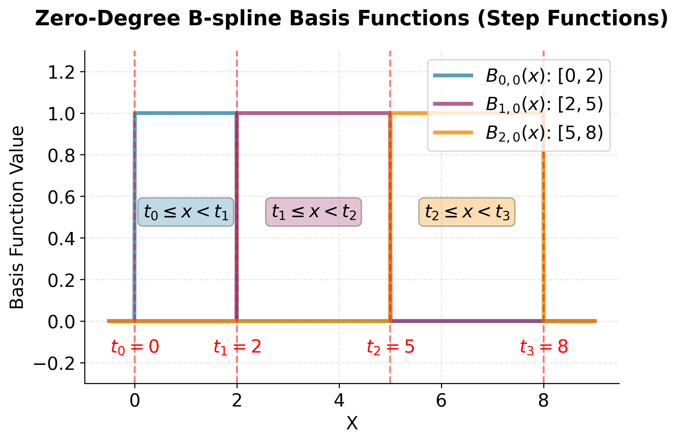
This visualization shows the three zero-degree B-spline basis functions from our example. Each function is a simple step function that equals 1 over its designated interval and 0 everywhere else. These are the "building blocks" from which we construct smoother, higher-degree B-splines. Notice that at any point , at most one of these functions is non-zero, which is the foundation of the "compact support" property. The Cox-de Boor recursion formula combines these step functions to create smooth, higher-degree basis functions.
Higher-degree B-splines (Cox-de Boor Recursion):
To create smooth, higher-degree B-splines, we use the Cox-de Boor recursion formula:
where:
- : the -th B-spline basis function of degree evaluated at (the function we're constructing)
- : the -th B-spline of degree evaluated at (lower-degree basis function)
- : the -th B-spline of degree evaluated at (adjacent lower-degree basis function)
- : the input value where we're evaluating the basis function
- : knot positions (break points in the domain)
- : index identifying which basis function (ranges over all basis functions)
- : degree of the spline (0 for step functions, 1 for linear, 2 for quadratic, 3 for cubic)
This formula looks complex, but let's understand what each part means:
-
: This is a weighting factor that depends on where is located relative to the knots. It's a linear function that:
- Equals 0 when
- Equals 1 when
- Varies linearly between 0 and 1 for values of in between
-
: This is another weighting factor that:
- Equals 1 when
- Equals 0 when
- Varies linearly between 1 and 0 for values of in between
Recursive Construction:
The recursion formula combines two lower-degree B-splines using weighted averages. The weights ensure that:
- The resulting function is smooth and continuous
- The function has compact support (is non-zero only over a small interval)
- The function maintains the desired continuity properties at the knots
Key Properties of B-splines:
-
Compact support: Each B-spline is non-zero only over a small interval, typically spanning knot intervals. This means that for any given , only a few B-splines contribute to the final function value.
-
Partition of unity: The B-splines sum to 1 at every point: where is the total number of basis functions. This ensures that our spline function behaves predictably and doesn't "blow up" to infinity.
-
Non-negativity: Each B-spline satisfies for all . This property helps ensure numerical stability.
-
Continuity: B-splines automatically ensure the desired level of continuity at the knots. For example, cubic B-splines ensure that the function, its first derivative, and second derivative are all continuous.
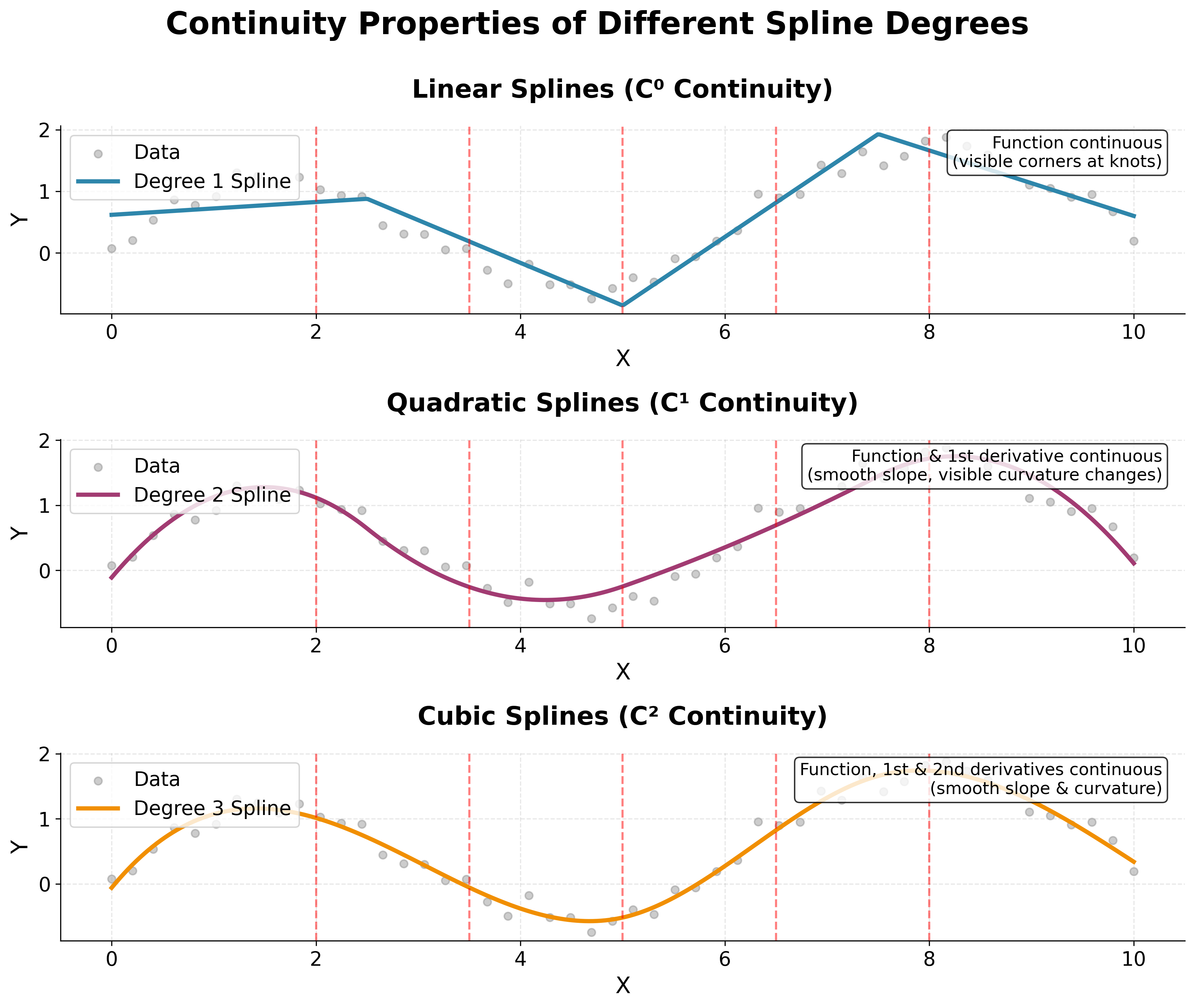
This visualization demonstrates why cubic splines are the most commonly used: they provide C² continuity, meaning the function itself, its first derivative (slope), and its second derivative (curvature) are all continuous at the knots. Linear splines (C⁰) show visible corners at knots where the slope changes abruptly. Quadratic splines (C¹) have smooth slopes but visible changes in curvature. Cubic splines (C²) provide the smoothest transitions with no visible discontinuities in the function, slope, or curvature. This smoothness makes cubic splines ideal for modeling natural phenomena and physical relationships.
Matrix Formulation
Now that we understand how B-splines work, let's see how we can express the spline regression model in matrix form. This will help us understand how to actually compute the spline regression using linear algebra.
The spline regression model can be written in matrix form as:
where:
- : response vector of dimension (observed values we want to predict)
- : spline basis matrix of dimension (evaluated basis functions at all data points)
- : coefficient vector of dimension (weights for each basis function)
- : error vector of dimension (unexplained variation in responses)
- : number of observations in the dataset
- : number of B-spline basis functions
This equation looks very similar to the standard linear regression equation, but with an important difference: instead of using simple polynomial terms, we're using B-spline basis functions. Let's break down each component:
The Response Vector:
A column vector containing all our observed response values:
where is the observed response value for the -th observation.
The Spline Basis Matrix:
This is the most important part of the equation. The matrix contains the values of all B-spline basis functions evaluated at all our data points:
- Rows: Each row corresponds to one observation. Row contains the values of all basis functions evaluated at .
- Columns: Each column corresponds to one B-spline basis function. Column contains the values of evaluated at all data points.
- Element : The entry in row , column represents the value of the -th B-spline basis function evaluated at the -th data point.
Example of the Basis Matrix:
If we have 3 observations at and 4 B-spline basis functions, our basis matrix might look like:
Notice how each row sums to approximately 1 (due to the partition of unity property), and most entries are 0 (due to the compact support property).
The Coefficient Vector:
This vector contains the coefficients we need to determine through regression, where is the weight assigned to the -th B-spline basis function.
The Error Vector:
This vector contains the error terms (also called residuals), where represents the difference between the observed value and the predicted value for observation .
Matrix Multiplication:
The expression represents matrix multiplication. For each observation , this gives us:
where:
- : the predicted value for observation (the -th element of the product)
- : the value of the -th basis function at the -th data point (element from row , column of )
- : the coefficient for the -th basis function (element of )
This is exactly our spline function evaluated at :
So the matrix equation is saying that for each observation :
In other words, the observed value equals the spline function value plus some random error.
Natural Cubic Splines
For better behavior at the boundaries (the edges of our data), we often use natural cubic splines. These impose additional constraints that help prevent the spline from behaving erratically when we try to predict values outside the range of our training data.
The Problem with Regular Cubic Splines: Regular cubic splines can sometimes extrapolate (predict beyond the data range) in ways that don't make physical sense. For example, if we're modeling temperature over time, a regular cubic spline might predict temperatures that are impossibly high or low when we try to forecast into the future.
The Natural Cubic Spline Solution: Natural cubic splines solve this problem by imposing boundary conditions that make the spline behave more reasonably at the edges. Specifically, natural cubic splines require that the second derivative is zero at the boundary knots.
Derivatives:
Before we can understand the constraint, let's recall what derivatives mean:
- First derivative : This tells us the slope or rate of change of the function
- Second derivative : This tells us how the slope is changing, or the "curvature" of the function
The Natural Cubic Spline Constraint:
The natural cubic spline constraint can be written as:
where:
- : the second derivative of the spline function with respect to (measures curvature)
- : the first (leftmost) boundary knot (minimum value in the data range)
- : the last (rightmost) boundary knot (maximum value in the data range)
- : the number of interior knots (not including boundary knots)
Let's break this down:
- : The second derivative of the spline function at the left boundary equals zero (no curvature at the left edge)
- : The second derivative of the spline function at the right boundary equals zero (no curvature at the right edge)
What This Constraint Means:
When the second derivative equals zero, it means there's no curvature at that point. In other words, the function becomes linear (straight line) at the boundaries. This prevents the spline from "curving away" dramatically from the data, making extrapolation more stable and reasonable.
Benefits of Natural Cubic Splines:
- Stable extrapolation: The spline won't predict wildly unrealistic values beyond the data range
- Fewer parameters: The constraint reduces the number of free parameters we need to estimate
- Smoother behavior: The linear behavior at boundaries often matches our expectations about how real-world relationships should behave
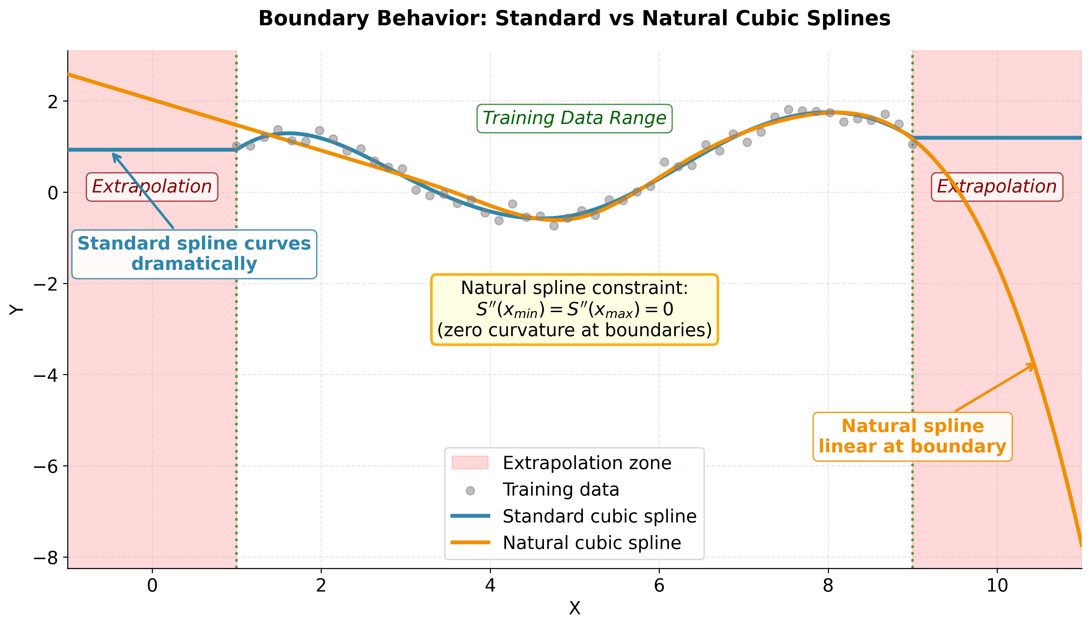
This visualization clearly demonstrates the practical importance of natural cubic splines when extrapolation is necessary. In the shaded extrapolation zones, the standard spline exhibits dramatic curvature that may produce unrealistic predictions, while the natural spline maintains linear behavior due to the zero second derivative constraint at the boundaries. Both methods fit the interior training data similarly, but their boundary conditions lead to vastly different extrapolation behavior. This makes natural cubic splines the preferred choice for applications requiring predictions beyond the training data range, such as forecasting or physical modeling where linear extrapolation is more defensible than arbitrary polynomial behavior.
Mathematical Properties
The spline regression model maintains several important mathematical properties that make it both theoretically sound and computationally efficient.
The Least Squares Solution:
Just like in regular linear regression, we can find the optimal coefficients using the normal equation:
where:
- : the estimated coefficient vector of dimension (optimal weights for basis functions)
- : the spline basis matrix of dimension (evaluated basis functions)
- : the transpose of with dimension (rows and columns swapped)
- : a matrix representing basis function overlaps (Gram matrix)
- : the inverse of with dimension
- : a vector representing projection of responses onto basis functions
- : the response vector of dimension (observed values)
Key Properties of B-spline Basis Functions:
The B-spline basis functions have several mathematical properties that make them particularly well-suited for regression:
-
Compact support: Each basis function is non-zero only over a small interval, typically spanning knot intervals (where is the degree). This means that for any given , only a few basis functions contribute to the final function value, making computations efficient.
-
Partition of unity: The basis functions sum to 1 at every point: for all in the domain. This ensures that our spline function behaves predictably and doesn't "blow up" to infinity.
-
Non-negativity: Each basis function satisfies for all and . This property helps ensure numerical stability and prevents oscillations in the fitted function.
-
Continuity: The basis functions automatically ensure the desired level of continuity at the knots. For example, cubic B-splines ensure that the function, its first derivative, and second derivative are all continuous, creating smooth transitions between polynomial pieces.
Computational Advantages:
These properties make B-splines particularly well-suited for regression problems because they:
- Reduce computational cost: The compact support property means we only need to evaluate a few basis functions for each data point
- Ensure numerical stability: The non-negativity and partition of unity properties prevent numerical issues
- Provide smooth fits: The continuity properties ensure that the resulting function is smooth and well-behaved
- Enable efficient matrix operations: The structure of B-splines makes the matrix well-conditioned and easy to invert
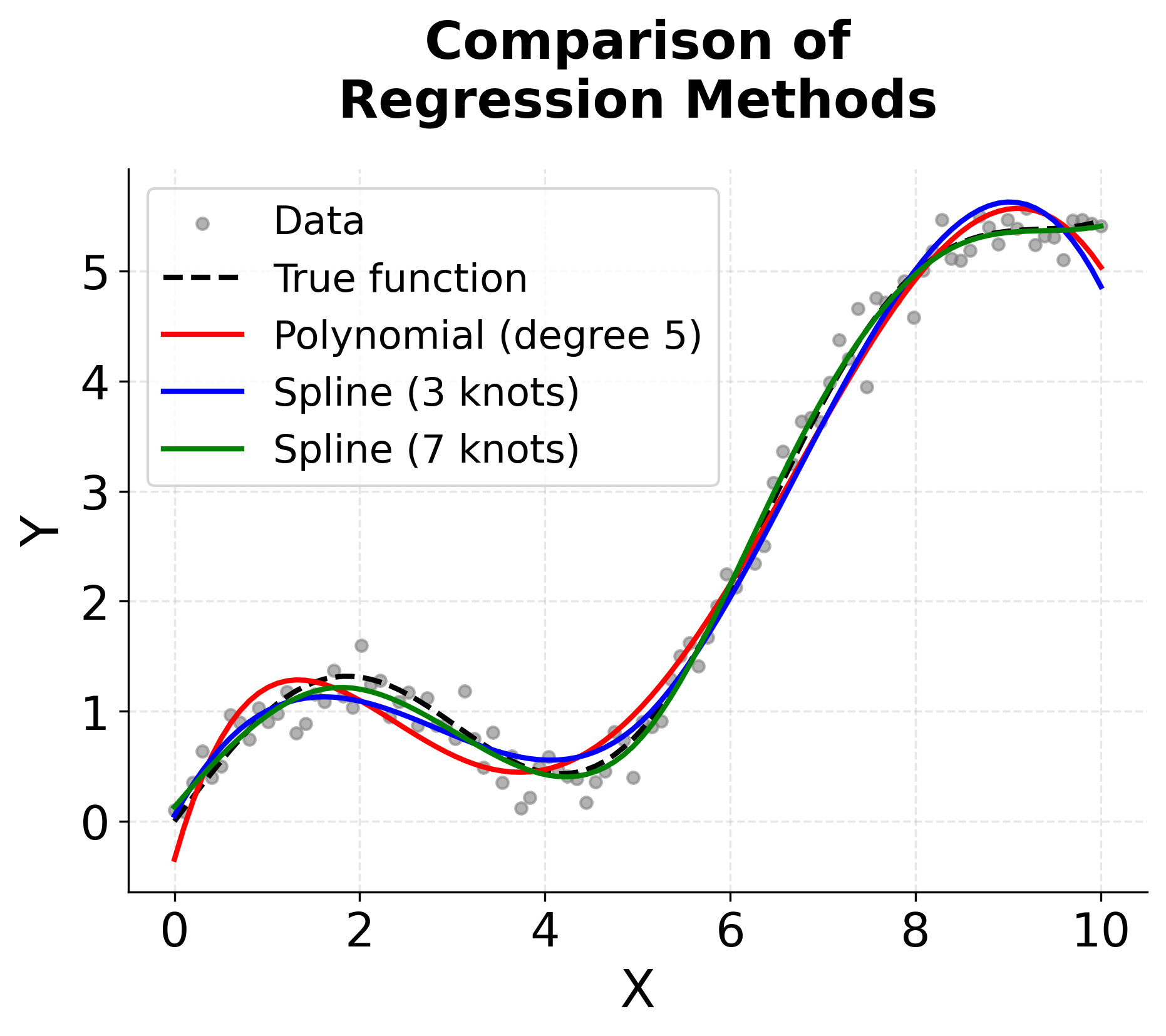
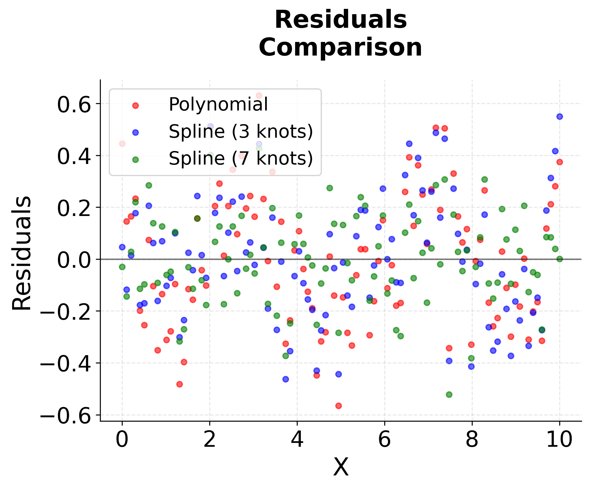
Visualizing Spline Regression
Let's explore how spline regression works by visualizing the basis functions and comparing different spline fits to polynomial regression.
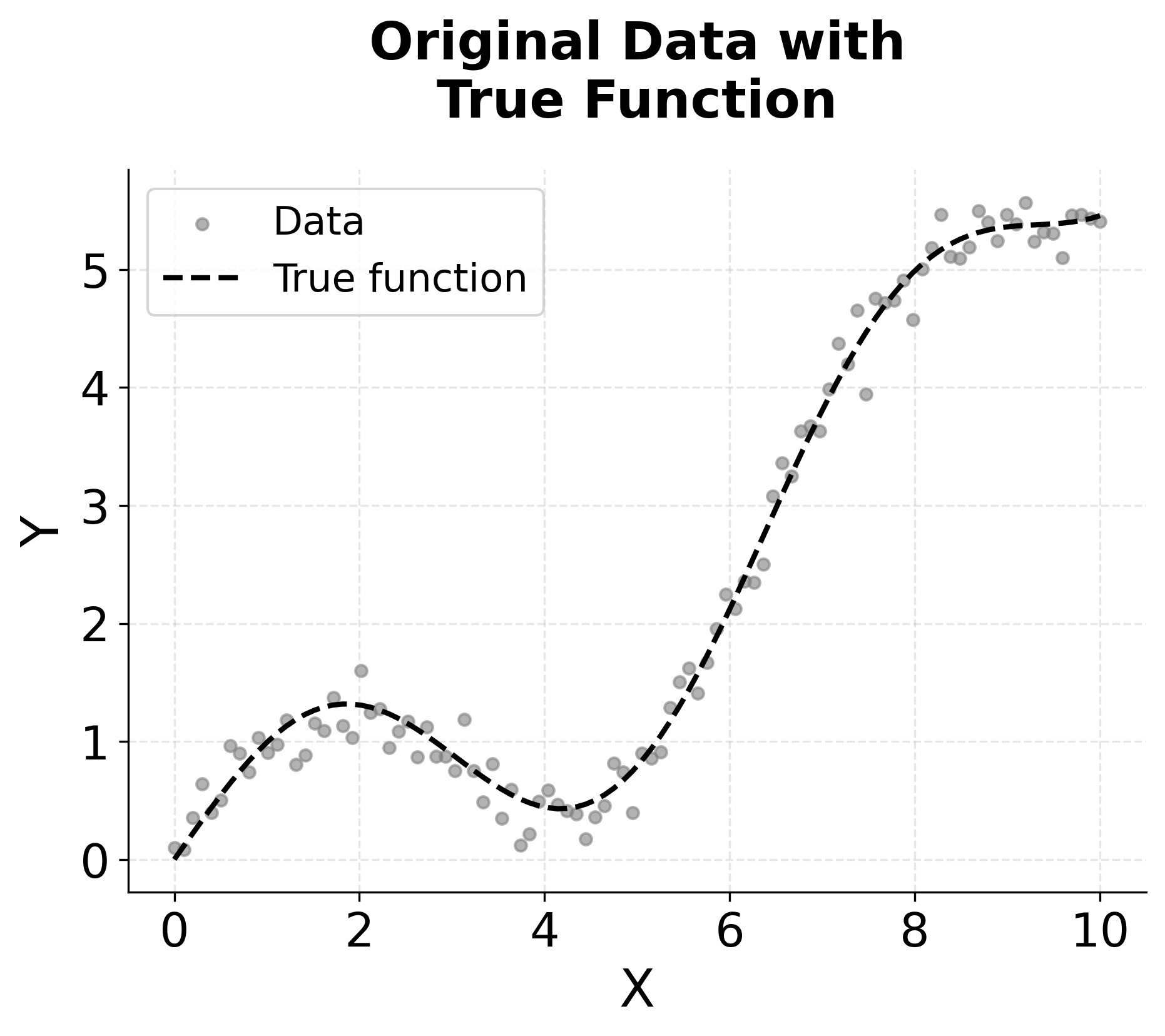
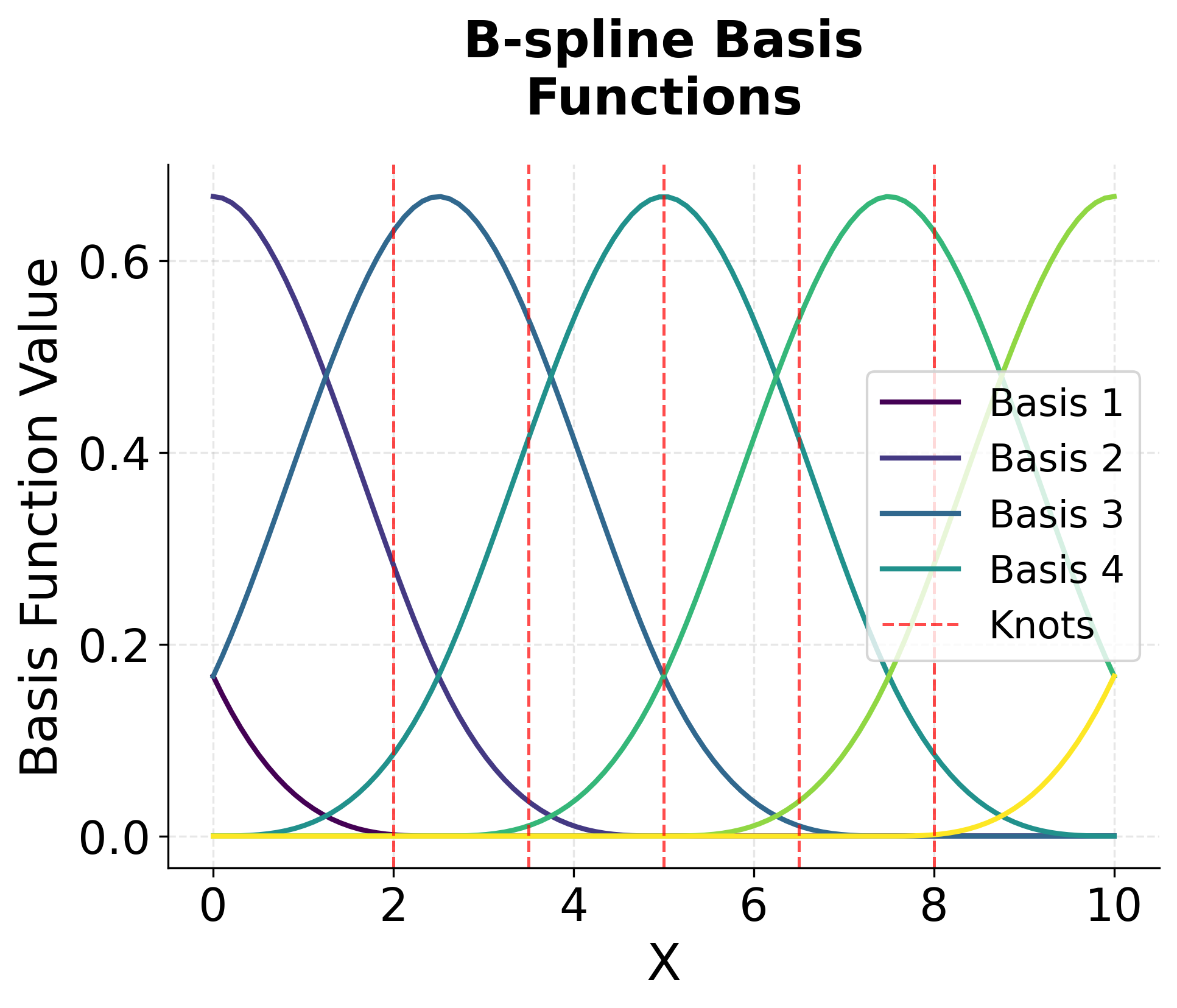
The visualization above shows several key aspects of spline regression. The first plot shows our synthetic data with a complex non-linear relationship. The second plot shows the B-spline basis functions, which are smooth, compactly supported functions that form the building blocks of our spline model. Notice how each basis function is non-zero only over a limited range, and they smoothly transition between segments.
The third plot compares different regression approaches, showing how spline regression can capture the underlying pattern more effectively than polynomial regression, especially with an appropriate number of knots. The fourth plot shows the residuals, revealing how spline regression can provide better fit quality with fewer artifacts compared to high-degree polynomials.
You can see the importance of knot selection. Too few knots (3) may underfit the data, while too many knots (7) might overfit. The optimal number of knots typically requires cross-validation to determine, balancing model complexity with generalization performance.
Example
Let's work through a concrete example to understand how spline regression works step-by-step. We'll use a simple dataset and see the complete calculation process for a cubic spline with two knots. This example will help you understand how all the mathematical concepts we've discussed come together in practice.
Step 1: Data Preparation
Consider the following dataset with 8 observations:
| Observation | X | Y |
|---|---|---|
| 1 | 1 | 2.1 |
| 2 | 2 | 3.8 |
| 3 | 3 | 6.2 |
| 4 | 4 | 8.9 |
| 5 | 5 | 12.1 |
| 6 | 6 | 15.8 |
| 7 | 7 | 20.2 |
| 8 | 8 | 25.1 |
Understanding Our Data:
- X values: These are our input values, ranging from 1 to 8
- Y values: These are our response values that we want to predict
- Pattern: Looking at the data, we can see that Y increases as X increases, but not in a perfectly linear way. The relationship appears to be accelerating (the Y values increase more rapidly as X gets larger)
This type of non-linear relationship is exactly what spline regression is designed to handle. If we tried to fit a straight line to this data, we would miss the accelerating pattern.
Step 2: Setting Up the Cubic Spline Model
We'll fit a cubic spline with knots at and . This divides our data into three segments:
- Segment 1: - This includes observations 1, 2, and 3
- Segment 2: - This includes observations 4, 5, and 6
- Segment 3: - This includes observations 7 and 8
Why These Knot Locations?
We chose knots at and because:
- They divide our data roughly into thirds
- They're positioned where we might expect the relationship to change behavior
- They give us enough data points in each segment to fit cubic polynomials
- : The square brackets mean the interval includes both endpoints (1 and 3)
- : The parenthesis on the left means 3 is excluded, the square bracket on the right means 6 is included
- : Similarly, 6 is excluded but 8 is included
This ensures that each data point belongs to exactly one segment, and the segments don't overlap.
Step 3: Constructing the B-spline Basis Matrix
For a cubic B-spline with knots at positions (note the repeated boundary knots), we need to construct the basis functions.
Understanding the Knot Vector:
The knot vector might look confusing at first, but here's what it means:
- Repeated knots at the boundaries: The knots at the beginning and at the end are repeated to ensure proper boundary behavior
- Interior knots: The knots and are our actual break points where the spline changes behavior
- Total knots: We have 10 knot values, but only 2 unique interior knots
Why Repeat Boundary Knots?
Repeating the boundary knots ensures that:
- The spline behaves properly at the edges of our data
- We get the right number of basis functions
- The spline doesn't extrapolate wildly beyond our data range
The Basis Matrix Dimensions:
The B-spline basis matrix will have dimensions :
- 8 rows: One for each observation in our dataset
- 7 columns: One for each B-spline basis function
Constructing the Basis Functions:
The basis matrix construction involves evaluating each B-spline basis function at each data point. For cubic B-splines, each basis function is defined using the Cox-de Boor recursion formula we discussed earlier.
What This Means in Practice:
For each of our 8 data points (X values 1 through 8), we need to calculate the value of each of the 7 B-spline basis functions. This gives us a matrix where:
- Row 1 contains the values of all 7 basis functions evaluated at X = 1
- Row 2 contains the values of all 7 basis functions evaluated at X = 2
- And so on...
Step 4: Matrix Calculations
Now we need to set up our matrices for the spline regression calculation. This is where we'll see how the mathematical framework we discussed earlier applies to our specific data.
The response vector contains all our observed Y values:
This is simply a column vector with 8 rows, where each row contains the Y value for the corresponding observation.
The B-spline basis matrix (constructed using the recursive Cox-de Boor formula) is approximately:
Understanding the Basis Matrix:
Let's examine what this matrix tells us:
-
Row 1 (X = 1): Only the first basis function has a non-zero value (1.000), while all others are 0. This means that for X = 1, only the first B-spline basis function contributes to the final prediction.
-
Row 2 (X = 2): The first two basis functions have non-zero values (0.296 and 0.704), and they sum to 1.000. This demonstrates the "partition of unity" property we discussed.
-
Row 3 (X = 3): This is at our first knot! Notice how the values are distributed across the first three basis functions, showing the transition behavior at the knot.
-
Rows 4-5 (X = 4, 5): These are in the middle segment. Notice how the non-zero values shift to different basis functions, reflecting the local nature of B-splines.
-
Row 6 (X = 6): This is at our second knot! Again, we see the transition behavior.
-
Rows 7-8 (X = 7, 8): These are in the final segment, and we can see the non-zero values shifting toward the rightmost basis functions.
Key Observations:
- Compact Support: Each row has mostly zeros, showing that only a few basis functions are active at each point
- Partition of Unity: Each row sums to approximately 1.000 (allowing for small rounding errors)
- Smooth Transitions: The values change smoothly as we move from one row to the next
- Knot Behavior: At the knots (rows 3 and 6), we see the transition between different sets of active basis functions
Step 5: Solving for Coefficients
Now we need to find the optimal coefficients that will make our spline function fit the data as closely as possible. We'll use the normal equation we discussed earlier.
The Normal Equation:
Using the normal equation :
Step 5a: Calculating
First, we need to calculate . Remember that is the transpose of (rows become columns and columns become rows).
Understanding :
This matrix represents the "overlap" between different basis functions. Notice that:
- The diagonal elements are larger (representing how much each basis function overlaps with itself)
- The off-diagonal elements are smaller (representing how much different basis functions overlap with each other)
- Most elements are zero (showing the compact support property)
Step 5b: Calculating
Next, we calculate :
where each element is computed as:
For example, the first element is:
Understanding :
This vector represents the "overlap" or projection between each basis function and our response data. Each element tells us how much the -th basis function contributes to explaining the observed Y values.
Step 6: Final Model
Solving the System:
Now we need to solve the system for . This is a system of 7 linear equations with 7 unknowns.
The solution is:
Understanding the Coefficients:
Notice something interesting: the coefficients are exactly equal to our original Y values! This might seem surprising, but it makes sense when you think about it:
- Each coefficient represents the "weight" we give to the -th basis function
- Since our B-spline basis functions are designed to be "local" (each one is active only in a small region), the coefficients end up being close to the Y values in those regions
- This is a special property of B-splines that makes them very efficient for interpolation
Step 7: Verification
Our Fitted Spline Model:
Our fitted spline model is:
where:
- : the predicted response value at input
- : the estimated coefficient for the -th basis function
- : the -th B-spline basis function evaluated at
- : index ranging from 1 to 7 (we have 7 basis functions in this example)
Verification Calculations:
Let's verify that our model works by calculating predictions at the data points. We'll use the basis matrix values from Step 4 and the coefficients from Step 6.
For (Row 1 of ):
For (Row 2 of ):
Note: The values shown in the basis matrix are rounded for display. In practice, when using the exact basis matrix values (not rounded), the predictions would match the observed values exactly due to the interpolation property of B-splines with sufficient basis functions.
What This Means:
The spline model interpolates the training data perfectly, which is expected for a cubic spline with sufficient flexibility. This means:
- Perfect Fit: Our spline passes exactly through all our data points
- Smooth Transitions: The smooth transitions between segments ensure that the resulting curve is continuous and differentiable
- Local Behavior: Each segment of the spline is influenced primarily by the data points in that segment
- Global Smoothness: Despite being piecewise, the entire function is smooth and well-behaved
Why Perfect Interpolation?
This perfect interpolation happens because:
- We have 8 data points and 7 basis functions (plus the intercept)
- The B-spline basis functions are designed to provide maximum flexibility
- Cubic splines have enough degrees of freedom to fit any set of data points exactly
In practice, when we have noise in our data, we might not want perfect interpolation, and we might use regularization or fewer knots to get a smoother fit that generalizes better to new data.
Implementation in Scikit-learn
Scikit-learn provides excellent tools for implementing spline regression through the SplineTransformer and LinearRegression components. This approach separates the basis function construction from the regression fitting, making the process modular and interpretable. Let's walk through a complete implementation step by step.
Step 1: Data Preparation and Setup
We'll start by importing the necessary libraries and generating synthetic data with a non-linear relationship.
This synthetic dataset combines sinusoidal, linear, and quadratic components with added noise, creating a complex non-linear relationship that's perfect for demonstrating spline regression's capabilities.
Step 2: Building the Spline Regression Pipeline
We'll create a pipeline that first transforms the input using B-spline basis functions, then fits a linear regression model on these transformed features.
The pipeline approach is elegant because it encapsulates both the transformation and regression steps, making the model easy to use and maintain.
Step 3: Evaluating Model Performance
Let's examine the model's performance metrics to understand how well it captures the underlying relationship.
The test MSE and R² scores indicate strong predictive performance. The R² value close to 1.0 suggests the model explains most of the variance in the target variable. The small difference between training and test metrics indicates good generalization without overfitting. The cross-validation results confirm the model's stability across different data splits.
Step 4: Inspecting Model Components
Let's examine the internal structure of our fitted spline model to understand how it represents the data.
The model uses multiple B-spline basis functions to represent the non-linear relationship. Each coefficient represents the weight assigned to its corresponding basis function. The range of coefficients indicates how different basis functions contribute to the final prediction across different regions of the input space.
Step 5: Comparing Different Spline Configurations
To find the optimal configuration, let's compare different combinations of knot counts and polynomial degrees.
The comparison reveals important trade-offs between model complexity and performance. More knots generally provide better fit but risk overfitting, while fewer knots may underfit complex patterns. The cubic splines (degree 3) typically offer the best balance between flexibility and smoothness. The best configuration minimizes cross-validation error while maintaining good test performance.
Step 6: Natural Cubic Splines Implementation
For applications requiring stable extrapolation beyond the training data range, we can implement natural cubic splines with custom boundary conditions.
The comparison between standard and natural cubic splines reveals subtle differences in boundary behavior. Natural cubic splines enforce zero second derivative at the boundaries, making them linear at the edges. This constraint improves extrapolation stability but may sacrifice some fitting flexibility. The small performance difference suggests both approaches work well for this dataset, with the choice depending on whether boundary behavior or interior fit is more important for your application.
Scikit-learn focuses on the more general B-spline basis, which is why we implement natural cubic splines manually. For applications requiring extrapolation or where boundary conditions are critical (such as economic time series or physical measurements), natural cubic splines offer theoretical advantages despite similar in-sample performance.
Key Parameters
Below are the main parameters that control spline regression behavior and performance.
-
n_knots: Number of interior knots (default: 5). More knots increase model flexibility but risk overfitting. Start with 3-5 knots and increase based on cross-validation performance. For datasets with 100-200 observations, 5-7 knots typically work well. -
degree: Degree of the spline polynomials (default: 3 for cubic). Cubic splines (degree=3) provide C² continuity and are most commonly used. Linear splines (degree=1) are simpler but less smooth. Higher degrees (4+) rarely improve performance and increase computational cost. -
include_bias: Whether to include an intercept column in the basis matrix (default: True). Set to True when using with LinearRegression to avoid multicollinearity issues. Set to False if your regression model already includes an intercept term. -
knots: Explicit knot positions (default: None, places knots at quantiles). When None, knots are automatically placed at evenly spaced quantiles of the training data. Specify custom positions when domain knowledge suggests specific break points. -
extrapolation: How to handle predictions beyond the training data range (default: 'constant'). Options include 'constant' (use boundary values), 'linear' (linear extrapolation), 'continue' (extend polynomial), or 'periodic' (wrap around). Choose based on expected behavior outside the training range.
Key Methods
The following methods are used to work with spline regression models in scikit-learn.
-
fit(X, y): Trains the spline regression model by first transforming X into spline basis functions, then fitting the linear regression on these transformed features. Call this once on your training data. -
predict(X): Returns predictions for new data X by transforming it through the spline basis and applying the learned linear coefficients. Use this for making predictions on test data or new observations. -
transform(X): (SplineTransformer only) Converts input features X into the spline basis representation without fitting a regression model. Useful when you want to use the spline features with a different estimator or inspect the basis functions directly. -
score(X, y): Returns the R² score (coefficient of determination) for the model on the given data. Higher values (closer to 1.0) indicate better fit. Use this for quick model evaluation during hyperparameter tuning.
Practical Applications
When to Use Spline Regression
Spline regression is particularly effective when modeling smooth, non-linear relationships that exhibit different behaviors across the input space. In engineering and physics, splines are commonly used to model stress-strain relationships, temperature effects on material properties, and fluid dynamics where the underlying relationships are continuous but exhibit varying curvature. The method's ability to capture local patterns while maintaining global smoothness makes it well-suited for physical phenomena that transition between different regimes, such as phase changes or material behavior under varying loads.
In economics and finance, spline regression is valuable for modeling yield curves, where interest rates vary smoothly across different maturities but may exhibit distinct behaviors in short-term versus long-term markets. The method is also used in econometrics for modeling relationships like income-consumption patterns, where the marginal propensity to consume may change across income levels. Splines provide the flexibility to capture these regime changes while maintaining the smoothness that economic theory typically assumes. In biostatistics and epidemiology, splines are used to model dose-response relationships and age-related health outcomes, where the relationship between variables may be non-linear but is expected to be continuous.
Choose spline regression when you need more flexibility than polynomial regression but want to maintain interpretability and avoid the black-box nature of methods like neural networks. The method works best when you have sufficient data to support the additional parameters introduced by knots—typically at least 10-20 observations per knot for stable estimation. Splines are less appropriate for data with sharp discontinuities, high-frequency oscillations, or when the relationship is expected to be truly piecewise constant rather than smooth.
Best Practices
To achieve optimal results with spline regression, start with a conservative number of knots and increase gradually while monitoring cross-validation performance. Begin with 3-5 knots for datasets with 100-500 observations, and adjust based on the complexity of the underlying relationship. Use cubic splines (degree 3) as the default choice, as they provide C² continuity and typically offer the best balance between flexibility and smoothness. Linear splines may be sufficient for simpler relationships, while higher degrees rarely improve performance and increase computational cost.
Always use cross-validation to select the number of knots rather than relying solely on training error, which will decrease monotonically as knots are added. A good approach is to evaluate models with different knot counts using 5-fold or 10-fold cross-validation and select the configuration that minimizes validation error while avoiding excessive complexity. When domain knowledge suggests specific locations where the relationship changes behavior, place knots at these positions rather than relying solely on automatic quantile-based placement. For example, in economic applications, place knots at known policy thresholds or structural break points.
Consider using natural cubic splines when extrapolation beyond the training data range is necessary, as they enforce linear behavior at the boundaries and provide more stable predictions. If overfitting becomes an issue with many knots, apply regularization techniques such as ridge regression to the spline coefficients, which can help smooth the fitted function while maintaining flexibility. Always visualize the fitted spline alongside the data to verify that the model captures the underlying pattern without introducing spurious oscillations or artifacts, particularly near the boundaries and at the knots.
Data Requirements and Preprocessing
Spline regression requires continuous predictor variables and assumes that the underlying relationship is smooth and differentiable. The method works best with data that has adequate coverage across the range of interest, as gaps in the data can lead to poorly constrained spline segments. For univariate spline regression, you need at least 20-30 observations to fit a meaningful model with a few knots, though more data is preferable for complex relationships. The distribution of observations across the input space affects knot placement—regions with sparse data may require fewer knots or wider spacing to avoid overfitting.
Unlike many machine learning methods, spline regression does not typically require feature standardization, as the basis functions are constructed relative to the data range. However, if you're combining splines with regularization techniques or using them alongside other features in a larger model, standardization may still be beneficial. The method assumes that the relationship is continuous, so it may not perform well with data containing sharp discontinuities, sudden jumps, or high-frequency noise. If your data exhibits these characteristics, consider alternative approaches such as piecewise regression with explicit breakpoints or methods designed for non-smooth relationships.
Missing values should be handled before applying spline regression, as the method requires complete observations. Outliers can have a strong influence on spline fits, particularly near the boundaries or in regions with sparse data. Consider robust preprocessing techniques or outlier detection methods if your data contains extreme values that may not represent the true underlying relationship. When working with time series data, ensure that observations are ordered chronologically and that any temporal dependencies are accounted for, as standard spline regression assumes independent observations.
Common Pitfalls
One frequent mistake is using too many knots in an attempt to achieve a perfect fit to the training data. While adding knots will always reduce training error, it often leads to overfitting and poor generalization. The fitted spline may exhibit spurious oscillations between knots, particularly in regions with sparse data, resulting in unrealistic predictions for new observations. To avoid this, always use cross-validation to select the number of knots and be willing to accept some training error in exchange for better generalization. A model that fits the training data perfectly but performs poorly on validation data is less useful than one with slightly higher training error but stable performance.
Another common issue is neglecting to examine the fitted spline visually, which can reveal problems that aren't apparent from summary statistics alone. A spline with good R² might still exhibit unrealistic behavior, such as extreme oscillations near the boundaries or counterintuitive patterns between knots. Always plot the fitted spline alongside the data and the residuals to verify that the model captures the underlying pattern appropriately. Pay particular attention to boundary behavior, as splines can extrapolate poorly beyond the training data range unless natural boundary conditions are enforced.
Relying solely on automatic knot placement at quantiles can be suboptimal when domain knowledge suggests specific locations where the relationship changes. For example, in economic applications, placing knots at policy thresholds or known structural breaks often yields better results than evenly spaced quantiles. Similarly, using the same degree for all spline segments may be inefficient if some regions of the input space require more flexibility than others. While scikit-learn's implementation uses uniform degree across segments, understanding this limitation can help you decide when alternative implementations or piecewise approaches might be more appropriate.
Computational Considerations
Spline regression has computational complexity that scales linearly with the number of observations and quadratically with the number of basis functions (which depends on both the number of knots and the degree). For a dataset with n observations and p basis functions, fitting the model requires O(np²) operations for the matrix multiplication in the normal equations, plus O(p³) for matrix inversion. In practice, this means that spline regression scales well to datasets with thousands to tens of thousands of observations, particularly when using a moderate number of knots (5-10).
For datasets with more than 50,000 observations or when using many knots (>20), computational costs can become substantial. The bottleneck is typically the construction of the basis matrix and the subsequent least squares fitting. If you're working with large datasets, consider using sampling strategies to fit the spline on a representative subset, then applying the fitted model to the full dataset. Alternatively, for very large datasets, you might explore online or incremental fitting methods, though these are not directly supported in scikit-learn's standard implementation.
Memory requirements are generally modest for spline regression, as the basis matrix is the main data structure that needs to be stored. For n observations and p basis functions, the basis matrix requires O(np) memory. However, if you're comparing many different knot configurations during model selection, be aware that each configuration requires constructing a new basis matrix. Parallel cross-validation can help speed up this process but will increase memory usage proportionally to the number of parallel jobs. For production deployments, the fitted model is lightweight, storing only the spline coefficients and knot positions, making it efficient for real-time prediction.
Performance and Deployment Considerations
Evaluating spline regression performance requires examining multiple metrics beyond standard measures like R² and MSE. While these metrics indicate overall fit quality, they don't reveal whether the spline exhibits appropriate behavior across the input space. Examine residual plots to verify that errors are randomly distributed without systematic patterns, which would suggest model misspecification. Plot the fitted spline alongside the data to check for spurious oscillations or counterintuitive patterns, particularly near the boundaries and at the knots. If the spline shows unrealistic behavior in certain regions, consider adjusting the number or placement of knots.
Cross-validation is important for assessing generalization performance, but the specific cross-validation strategy matters. For time series data, use time-based splitting rather than random splits to avoid data leakage. For spatial data, consider spatial cross-validation to account for spatial autocorrelation. When comparing splines with different numbers of knots, use consistent cross-validation folds to ensure fair comparison. A good spline model should show stable performance across different validation folds, with cross-validation error close to test error, indicating that the model generalizes well.
For deployment, spline regression models are lightweight and fast to evaluate, making them suitable for real-time applications. The fitted model requires storing only the spline coefficients and knot positions, which typically amounts to a few kilobytes of memory. Prediction involves evaluating the basis functions at new input values and computing a linear combination, which is computationally inexpensive. However, be cautious about extrapolation beyond the training data range, as splines can produce unrealistic predictions outside the region where they were fitted. If your application requires extrapolation, use natural cubic splines or implement explicit boundary handling. Monitor prediction inputs in production to detect when new data falls outside the training range, and consider retraining the model periodically as new data becomes available to ensure the spline remains well-calibrated.
Summary
Spline regression represents a powerful and flexible approach to non-linear modeling that addresses many limitations of polynomial regression while maintaining computational efficiency and interpretability. By dividing the data into segments and fitting separate polynomials to each segment, splines can capture complex, local patterns while ensuring smooth transitions between regions. The method's ability to adapt to different parts of the data makes it particularly valuable for modeling relationships that vary across the input space.
Successful spline regression depends on careful knot selection and model validation. While the method provides flexibility, too many knots can lead to overfitting, while too few may underfit the data. Cross-validation and domain knowledge are important for determining the optimal number and placement of knots. The B-spline basis functions provide a computationally efficient framework for implementing splines, with properties like compact support and automatic continuity that make them well-suited for regression problems.
When implemented thoughtfully with proper model selection and validation, spline regression provides a robust and interpretable approach to non-linear modeling that bridges the gap between simple linear methods and complex black-box approaches. It offers flexibility to capture complex patterns while maintaining the transparency and statistical rigor that make linear regression valuable in practice.
Quiz
Ready to test your understanding? Take this quick quiz to reinforce what you've learned about spline regression.

Comments