Market Microstructure: Order Books & Execution Mechanics

Michael Brenndoerfer

Quantitative Finance algorithmic-trading market-mechanics

Explore market microstructure mechanics including order book architecture, matching algorithms, and order types. Master liquidity analysis and execution logic.

Reading Level

Choose your expertise level to adjust how many terms are explained. Beginners see more tooltips, experts see fewer to maintain reading flow. Hover over underlined terms for instant definitions.

Market Microstructure and Order TypesLink Copied

When you submit an order to buy 1,000 shares of Apple, what actually happens? The answer is far more complex than "someone sells it to you." Your order enters an intricate ecosystem of competing exchanges, order books, matching engines, and execution protocols that determine not just whether your trade executes, but at what price, in what sequence, and with what impact on subsequent prices.

Market microstructure is the study of how trades are executed and prices are formed at the granular level. While traditional finance often treats markets as frictionless, assuming you can buy or sell any quantity at the current price, reality is messier. Orders queue in electronic order books, compete for execution priority, and leave footprints that move prices. Understanding these mechanics is essential for you to translate theoretical strategies into actual executed positions.

Building on our discussion of transaction costs and market impact in the previous chapter, we now examine the underlying plumbing: the order book architecture that determines execution, the taxonomy of order types available to traders, and the rules that govern how orders interact. This knowledge directly informs the execution algorithms we'll develop in the next chapter on optimal execution.

The Order BookLink Copied

The order book is the central mechanism through which modern electronic markets operate. It's a real-time record of all outstanding buy and sell orders for a security, organized by price level and arrival time.

Structure of the Order BookLink Copied

Before diving into the technical definition, it helps to understand what problem the order book solves. In any market, buyers and sellers rarely arrive at exactly the same moment with perfectly matching quantities and prices. Someone who wants to sell 500 shares right now may not find a buyer willing to take exactly 500 shares at that exact instant. The order book solves this coordination problem by serving as a persistent record of trading interest, allowing buyers and sellers to express their willingness to trade at specific prices and wait for counterparties to arrive.

Order Book

An order book is a list of all outstanding limit orders to buy (bids) and sell (asks/offers) a security organized by price level. It represents the current supply and demand for immediate execution at each price point.

The order book has two sides: the bid side contains all buy orders, and the ask side (or offer side) contains all sell orders. Orders on each side are sorted by price, with the most aggressive prices at the top. The highest bid is called the best bid, and the lowest ask is called the best ask (or best offer). The difference between these two prices is the bid-ask spread.

To quantify the key features of the order book, we define two fundamental measures that traders constantly monitor. The spread captures the cost of trading immediately, while the midprice provides a reference point for the security's theoretical fair value. These quantities are defined mathematically as follows:

\begin{aligned} S &= P_a - P_b \\ M &= \frac{P_a + P_b}{2} \end{aligned}

Let us examine each component of these formulas to understand their economic meaning:

$P_a$ : best ask price (lowest price to buy). This represents the minimum price at which someone in the market is currently willing to sell. If you want to buy immediately, this is the price you will pay.
$P_b$ : best bid price (highest price to sell). This represents the maximum price at which someone is currently willing to buy. If you want to sell immediately, this is the price you will receive.
$S$ : bid-ask spread, representing the cost of immediacy. The spread is always non-negative in a properly functioning market, since the best ask must be at least as high as the best bid (otherwise orders would immediately cross and execute). A narrow spread indicates a liquid market where trading is cheap, while a wide spread suggests illiquidity or uncertainty.
$M$ : midprice, representing the theoretical fair value. The midprice sits exactly halfway between the best bid and ask, and we often use it as a reference point for the "true" price of the security. However, the midprice is not a price at which you can actually trade; it is merely a convenient benchmark.

In[2]:

Code

from dataclasses import dataclass
from enum import Enum


# Define order side
class Side(Enum):
    BID = "bid"
    ASK = "ask"


@dataclass
class Order:
    """Represents a single order in the order book."""

    order_id: int
    side: Side
    price: float
    quantity: int
    timestamp: float  # seconds since epoch

    def __repr__(self):
        return f"Order({self.order_id}, {self.side.value}, ${self.price:.2f}, {self.quantity} shares)"

from dataclasses import dataclass
from enum import Enum


# Define order side
class Side(Enum):
    BID = "bid"
    ASK = "ask"


@dataclass
class Order:
    """Represents a single order in the order book."""

    order_id: int
    side: Side
    price: float
    quantity: int
    timestamp: float  # seconds since epoch

    def __repr__(self):
        return f"Order({self.order_id}, {self.side.value}, ${self.price:.2f}, {self.quantity} shares)"

Let's create a simple order book class that captures the essential mechanics:

In[3]:

Code

from collections import defaultdict
from typing import List, Tuple, Optional
from dataclasses import dataclass
from enum import Enum


# Re-import/define Side and Order for this cell
class Side(Enum):
    BID = "bid"
    ASK = "ask"


@dataclass
class Order:
    """Represents a single order in the order book."""

    order_id: int
    side: Side
    price: float
    quantity: int
    timestamp: float

    def __repr__(self):
        return f"Order({self.order_id}, {self.side.value}, ${self.price:.2f}, {self.quantity} shares)"


class OrderBook:
    """A simple limit order book implementation."""

    def __init__(self, ticker: str):
        self.ticker = ticker
        self.bids = defaultdict(list)  # price -> list of orders
        self.asks = defaultdict(list)  # price -> list of orders
        self.order_id_counter = 0
        self.current_time = 0.0

    def add_limit_order(self, side: Side, price: float, quantity: int) -> Order:
        """Add a limit order to the book."""
        self.order_id_counter += 1
        order = Order(
            order_id=self.order_id_counter,
            side=side,
            price=price,
            quantity=quantity,
            timestamp=self.current_time,
        )

        if side == Side.BID:
            self.bids[price].append(order)
        else:
            self.asks[price].append(order)

        self.current_time += 0.001  # increment time
        return order

    def get_best_bid(self) -> Optional[float]:
        """Return the highest bid price."""
        if not self.bids:
            return None
        return max(self.bids.keys())

    def get_best_ask(self) -> Optional[float]:
        """Return the lowest ask price."""
        if not self.asks:
            return None
        return min(self.asks.keys())

    def get_spread(self) -> Optional[float]:
        """Return the bid-ask spread."""
        best_bid = self.get_best_bid()
        best_ask = self.get_best_ask()
        if best_bid is None or best_ask is None:
            return None
        return best_ask - best_bid

    def get_midprice(self) -> Optional[float]:
        """Return the midpoint between best bid and ask."""
        best_bid = self.get_best_bid()
        best_ask = self.get_best_ask()
        if best_bid is None or best_ask is None:
            return None
        return (best_bid + best_ask) / 2

    def get_depth_at_price(self, side: Side, price: float) -> int:
        """Return total quantity at a given price level."""
        orders = self.bids[price] if side == Side.BID else self.asks[price]
        return sum(o.quantity for o in orders)

    def get_book_snapshot(self, levels: int = 5) -> Tuple[List, List]:
        """Return top N levels of bids and asks."""
        bid_prices = sorted(self.bids.keys(), reverse=True)[:levels]
        ask_prices = sorted(self.asks.keys())[:levels]

        bid_levels = [
            (p, self.get_depth_at_price(Side.BID, p)) for p in bid_prices
        ]
        ask_levels = [
            (p, self.get_depth_at_price(Side.ASK, p)) for p in ask_prices
        ]

        return bid_levels, ask_levels

from collections import defaultdict
from typing import List, Tuple, Optional
from dataclasses import dataclass
from enum import Enum


# Re-import/define Side and Order for this cell
class Side(Enum):
    BID = "bid"
    ASK = "ask"


@dataclass
class Order:
    """Represents a single order in the order book."""

    order_id: int
    side: Side
    price: float
    quantity: int
    timestamp: float

    def __repr__(self):
        return f"Order({self.order_id}, {self.side.value}, ${self.price:.2f}, {self.quantity} shares)"


class OrderBook:
    """A simple limit order book implementation."""

    def __init__(self, ticker: str):
        self.ticker = ticker
        self.bids = defaultdict(list)  # price -> list of orders
        self.asks = defaultdict(list)  # price -> list of orders
        self.order_id_counter = 0
        self.current_time = 0.0

    def add_limit_order(self, side: Side, price: float, quantity: int) -> Order:
        """Add a limit order to the book."""
        self.order_id_counter += 1
        order = Order(
            order_id=self.order_id_counter,
            side=side,
            price=price,
            quantity=quantity,
            timestamp=self.current_time,
        )

        if side == Side.BID:
            self.bids[price].append(order)
        else:
            self.asks[price].append(order)

        self.current_time += 0.001  # increment time
        return order

    def get_best_bid(self) -> Optional[float]:
        """Return the highest bid price."""
        if not self.bids:
            return None
        return max(self.bids.keys())

    def get_best_ask(self) -> Optional[float]:
        """Return the lowest ask price."""
        if not self.asks:
            return None
        return min(self.asks.keys())

    def get_spread(self) -> Optional[float]:
        """Return the bid-ask spread."""
        best_bid = self.get_best_bid()
        best_ask = self.get_best_ask()
        if best_bid is None or best_ask is None:
            return None
        return best_ask - best_bid

    def get_midprice(self) -> Optional[float]:
        """Return the midpoint between best bid and ask."""
        best_bid = self.get_best_bid()
        best_ask = self.get_best_ask()
        if best_bid is None or best_ask is None:
            return None
        return (best_bid + best_ask) / 2

    def get_depth_at_price(self, side: Side, price: float) -> int:
        """Return total quantity at a given price level."""
        orders = self.bids[price] if side == Side.BID else self.asks[price]
        return sum(o.quantity for o in orders)

    def get_book_snapshot(self, levels: int = 5) -> Tuple[List, List]:
        """Return top N levels of bids and asks."""
        bid_prices = sorted(self.bids.keys(), reverse=True)[:levels]
        ask_prices = sorted(self.asks.keys())[:levels]

        bid_levels = [
            (p, self.get_depth_at_price(Side.BID, p)) for p in bid_prices
        ]
        ask_levels = [
            (p, self.get_depth_at_price(Side.ASK, p)) for p in ask_prices
        ]

        return bid_levels, ask_levels

Now let's populate an order book with some sample orders and visualize it:

In[4]:

Code

import numpy as np

# Create an order book for a hypothetical stock
book = OrderBook("XYZ")

# Add bid orders (buyers)
np.random.seed(42)
for price in [99.90, 99.85, 99.80, 99.75, 99.70]:
    for _ in range(np.random.randint(2, 6)):
        qty = np.random.randint(100, 1000)
        book.add_limit_order(Side.BID, price, qty)

# Add ask orders (sellers)
for price in [100.00, 100.05, 100.10, 100.15, 100.20]:
    for _ in range(np.random.randint(2, 6)):
        qty = np.random.randint(100, 1000)
        book.add_limit_order(Side.ASK, price, qty)

# Get the snapshot
bid_levels, ask_levels = book.get_book_snapshot(levels=5)

import numpy as np

# Create an order book for a hypothetical stock
book = OrderBook("XYZ")

# Add bid orders (buyers)
np.random.seed(42)
for price in [99.90, 99.85, 99.80, 99.75, 99.70]:
    for _ in range(np.random.randint(2, 6)):
        qty = np.random.randint(100, 1000)
        book.add_limit_order(Side.BID, price, qty)

# Add ask orders (sellers)
for price in [100.00, 100.05, 100.10, 100.15, 100.20]:
    for _ in range(np.random.randint(2, 6)):
        qty = np.random.randint(100, 1000)
        book.add_limit_order(Side.ASK, price, qty)

# Get the snapshot
bid_levels, ask_levels = book.get_book_snapshot(levels=5)

Out[5]:

Console

Order Book for XYZ
==================================================
Best Bid: $99.90
Best Ask: $100.00
Spread: $0.10
Midprice: $99.95

Top 5 Bid Levels:
  $99.90: 2,071 shares
  $99.85: 2,421 shares
  $99.80: 1,647 shares
  $99.75: 3,133 shares
  $99.70: 1,547 shares

Top 5 Ask Levels:
  $100.00: 1,152 shares
  $100.05: 972 shares
  $100.10: 2,155 shares
  $100.15: 732 shares
  $100.20: 3,037 shares

The order book reveals several key pieces of information. The spread of $0.10 represents the cost of immediacy: if you want to buy immediately, you pay the ask ($100.00), but if you're willing to wait, you could place a bid at $99.90. The depth at each level shows how much liquidity is available before the price moves to the next level.

Visualizing Order Book DepthLink Copied

A depth chart provides an intuitive visualization of the order book, showing cumulative volume at each price level:

In[6]:

Code

def plot_order_book_depth(book: OrderBook, levels: int = 10):
    """Create a depth chart visualization of the order book."""

    # Get all price levels
    bid_prices = sorted(book.bids.keys(), reverse=True)
    ask_prices = sorted(book.asks.keys())

    # Calculate cumulative depth
    bid_cumulative = []
    cumsum = 0
    for p in bid_prices:
        cumsum += book.get_depth_at_price(Side.BID, p)
        bid_cumulative.append((p, cumsum))

    ask_cumulative = []
    cumsum = 0
    for p in ask_prices:
        cumsum += book.get_depth_at_price(Side.ASK, p)
        ask_cumulative.append((p, cumsum))

    plt.rcParams.update(
        {
            "figure.figsize": (6.0, 4.0),
            "font.size": 10,
            "axes.titlesize": 11,
            "axes.labelsize": 10,
            "xtick.labelsize": 9,
            "ytick.labelsize": 9,
            "legend.fontsize": 9,
        }
    )
    fig, ax = plt.subplots()

    # Plot bids (green, left side)
    if bid_cumulative:
        bid_prices_plot = [x[0] for x in bid_cumulative]
        bid_depths = [x[1] for x in bid_cumulative]
        ax.fill_between(
            bid_prices_plot, bid_depths, alpha=0.3, color="green", step="post"
        )
        ax.step(
            bid_prices_plot,
            bid_depths,
            where="post",
            color="green",
            linewidth=2,
            label="Bids",
        )

    # Plot asks (red, right side)
    if ask_cumulative:
        ask_prices_plot = [x[0] for x in ask_cumulative]
        ask_depths = [x[1] for x in ask_cumulative]
        ax.fill_between(
            ask_prices_plot, ask_depths, alpha=0.3, color="red", step="post"
        )
        ax.step(
            ask_prices_plot,
            ask_depths,
            where="post",
            color="red",
            linewidth=2,
            label="Asks",
        )

    # Mark the spread
    best_bid = book.get_best_bid()
    best_ask = book.get_best_ask()
    ax.axvline(x=best_bid, color="green", linestyle="--", alpha=0.5)
    ax.axvline(x=best_ask, color="red", linestyle="--", alpha=0.5)
    ax.axvspan(best_bid, best_ask, alpha=0.1, color="gray", label="Spread")

    ax.set_xlabel("Price ($)")
    ax.set_ylabel("Cumulative Volume (shares)")
    ax.set_title(f"{book.ticker} Order Book Depth")
    ax.legend(loc="upper right")
    ax.grid(True, alpha=0.3)

    plt.show()

def plot_order_book_depth(book: OrderBook, levels: int = 10):
    """Create a depth chart visualization of the order book."""

    # Get all price levels
    bid_prices = sorted(book.bids.keys(), reverse=True)
    ask_prices = sorted(book.asks.keys())

    # Calculate cumulative depth
    bid_cumulative = []
    cumsum = 0
    for p in bid_prices:
        cumsum += book.get_depth_at_price(Side.BID, p)
        bid_cumulative.append((p, cumsum))

    ask_cumulative = []
    cumsum = 0
    for p in ask_prices:
        cumsum += book.get_depth_at_price(Side.ASK, p)
        ask_cumulative.append((p, cumsum))

    plt.rcParams.update(
        {
            "figure.figsize": (6.0, 4.0),
            "font.size": 10,
            "axes.titlesize": 11,
            "axes.labelsize": 10,
            "xtick.labelsize": 9,
            "ytick.labelsize": 9,
            "legend.fontsize": 9,
        }
    )
    fig, ax = plt.subplots()

    # Plot bids (green, left side)
    if bid_cumulative:
        bid_prices_plot = [x[0] for x in bid_cumulative]
        bid_depths = [x[1] for x in bid_cumulative]
        ax.fill_between(
            bid_prices_plot, bid_depths, alpha=0.3, color="green", step="post"
        )
        ax.step(
            bid_prices_plot,
            bid_depths,
            where="post",
            color="green",
            linewidth=2,
            label="Bids",
        )

    # Plot asks (red, right side)
    if ask_cumulative:
        ask_prices_plot = [x[0] for x in ask_cumulative]
        ask_depths = [x[1] for x in ask_cumulative]
        ax.fill_between(
            ask_prices_plot, ask_depths, alpha=0.3, color="red", step="post"
        )
        ax.step(
            ask_prices_plot,
            ask_depths,
            where="post",
            color="red",
            linewidth=2,
            label="Asks",
        )

    # Mark the spread
    best_bid = book.get_best_bid()
    best_ask = book.get_best_ask()
    ax.axvline(x=best_bid, color="green", linestyle="--", alpha=0.5)
    ax.axvline(x=best_ask, color="red", linestyle="--", alpha=0.5)
    ax.axvspan(best_bid, best_ask, alpha=0.1, color="gray", label="Spread")

    ax.set_xlabel("Price ($)")
    ax.set_ylabel("Cumulative Volume (shares)")
    ax.set_title(f"{book.ticker} Order Book Depth")
    ax.legend(loc="upper right")
    ax.grid(True, alpha=0.3)

    plt.show()

Out[7]:

Visualization

Step chart with green bid curve on left and red ask curve on right, showing cumulative order book depth. — Cumulative depth of the limit order book for the simulated asset. The green (bid) and red (ask) curves show available volume at each price level, with the gap between them representing the bid-ask spread and the slope indicating market depth.

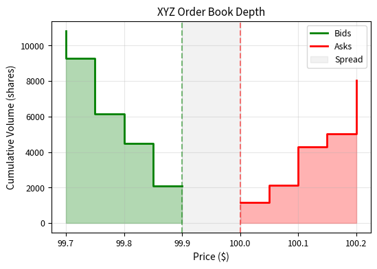
The depth chart shows how much buying power exists at each price level below the current price (bids) and how much selling pressure exists above (asks). The steeper the curve, the more liquidity is concentrated near the best prices. Shallow curves indicate thin markets where even modest order sizes can move prices significantly.

Order TypesLink Copied

Understanding order types is crucial for implementing trading strategies effectively. Each order type serves a specific purpose and carries different execution characteristics and risks.

Market OrdersLink Copied

The most fundamental question a trader faces is whether to trade now or wait. Market orders represent the choice to trade immediately, accepting whatever price the market offers in exchange for certain execution. This trade-off between price and certainty lies at the heart of all order type decisions.

Market Order

A market order is an instruction to buy or sell immediately at the best available price. Market orders guarantee execution (in liquid markets) but not the execution price.

Market orders are the simplest order type: you want to trade now, regardless of price. When you submit a market buy order, it executes against the best available ask prices in the order book, consuming liquidity until your order is filled. The execution process follows the order book's price levels sequentially: your order first takes all available shares at the best ask, then moves to the next price level if more shares are needed, and continues until completely filled.

The key characteristics of market orders include:

Immediate execution: Your order fills right away against standing limit orders
Price uncertainty: The execution price depends on available liquidity
Liquidity consumption: You remove liquidity from the order book, typically paying a fee
Slippage risk: Large orders may walk through multiple price levels

The slippage risk deserves particular attention. When your order size exceeds the available quantity at the best price, you experience slippage: the average execution price differs from the initial best price. This is not a market malfunction; it is the natural consequence of consuming multiple price levels to complete a large order.

Let's implement market order execution in our order book:

In[8]:

Code

def execute_market_order(
    book: OrderBook, side: Side, quantity: int
) -> List[Tuple[float, int]]:
    """
    Execute a market order against the book.
    Returns list of (price, quantity) fills.
    """
    fills = []
    remaining = quantity

    # Determine which side of the book to hit
    if side == Side.BID:  # Buying - hit the asks
        price_levels = sorted(book.asks.keys())
        target_book = book.asks
    else:  # Selling - hit the bids
        price_levels = sorted(book.bids.keys(), reverse=True)
        target_book = book.bids

    for price in price_levels:
        if remaining <= 0:
            break

        orders_at_price = target_book[price]
        i = 0
        while i < len(orders_at_price) and remaining > 0:
            order = orders_at_price[i]
            fill_qty = min(order.quantity, remaining)
            fills.append((price, fill_qty))

            remaining -= fill_qty
            order.quantity -= fill_qty

            if order.quantity == 0:
                orders_at_price.pop(i)
            else:
                i += 1

        # Clean up empty price levels
        if not orders_at_price:
            del target_book[price]

    return fills

def execute_market_order(
    book: OrderBook, side: Side, quantity: int
) -> List[Tuple[float, int]]:
    """
    Execute a market order against the book.
    Returns list of (price, quantity) fills.
    """
    fills = []
    remaining = quantity

    # Determine which side of the book to hit
    if side == Side.BID:  # Buying - hit the asks
        price_levels = sorted(book.asks.keys())
        target_book = book.asks
    else:  # Selling - hit the bids
        price_levels = sorted(book.bids.keys(), reverse=True)
        target_book = book.bids

    for price in price_levels:
        if remaining <= 0:
            break

        orders_at_price = target_book[price]
        i = 0
        while i < len(orders_at_price) and remaining > 0:
            order = orders_at_price[i]
            fill_qty = min(order.quantity, remaining)
            fills.append((price, fill_qty))

            remaining -= fill_qty
            order.quantity -= fill_qty

            if order.quantity == 0:
                orders_at_price.pop(i)
            else:
                i += 1

        # Clean up empty price levels
        if not orders_at_price:
            del target_book[price]

    return fills

Let's see how a market order executes and potentially walks through multiple price levels:

In[9]:

Code

# Create a fresh order book
book = OrderBook("XYZ")

# Build the order book with known quantities
book.add_limit_order(Side.ASK, 100.00, 500)
book.add_limit_order(Side.ASK, 100.00, 300)
book.add_limit_order(Side.ASK, 100.05, 400)
book.add_limit_order(Side.ASK, 100.10, 600)

book.add_limit_order(Side.BID, 99.95, 400)
book.add_limit_order(Side.BID, 99.90, 500)

# Capture state before execution
best_ask_before = book.get_best_ask()

# Execute a large market buy order
market_buy_qty = 1500
fills = execute_market_order(book, Side.BID, market_buy_qty)

# Calculate execution statistics
total_qty = sum(qty for _, qty in fills)
total_cost = sum(price * qty for price, qty in fills)
avg_price = total_cost / total_qty if total_qty > 0 else 0

# Create a fresh order book
book = OrderBook("XYZ")

# Build the order book with known quantities
book.add_limit_order(Side.ASK, 100.00, 500)
book.add_limit_order(Side.ASK, 100.00, 300)
book.add_limit_order(Side.ASK, 100.05, 400)
book.add_limit_order(Side.ASK, 100.10, 600)

book.add_limit_order(Side.BID, 99.95, 400)
book.add_limit_order(Side.BID, 99.90, 500)

# Capture state before execution
best_ask_before = book.get_best_ask()

# Execute a large market buy order
market_buy_qty = 1500
fills = execute_market_order(book, Side.BID, market_buy_qty)

# Calculate execution statistics
total_qty = sum(qty for _, qty in fills)
total_cost = sum(price * qty for price, qty in fills)
avg_price = total_cost / total_qty if total_qty > 0 else 0

Out[10]:

Console

Market Buy Order: 1500 shares
========================================

Execution Fills:
  500 shares @ $100.00
  300 shares @ $100.00
  400 shares @ $100.05
  300 shares @ $100.10

Total Filled: 1,500 shares
Average Price: $100.0333
Best Ask Before: $100.00
Slippage: $0.0333 per share

The market order walked through three price levels to fill completely. Starting at the best ask of $100.00, it consumed 800 shares, then moved to $100.05 for another 400 shares, and finally took 300 shares at $100.10. This price impact is exactly what we analyzed in the previous chapter on transaction costs.

Limit OrdersLink Copied

If market orders represent the choice to trade immediately, limit orders represent the opposite choice: patience in exchange for price control. A limit order says "I am willing to trade, but only at a price I consider acceptable." This patience comes with a cost, since there is no guarantee the market will ever reach your price.

Limit Order

A limit order is an instruction to buy at or below a specified price (limit buy) or sell at or above a specified price (limit sell). Limit orders guarantee the execution price but not execution itself.

Limit orders provide price protection at the cost of execution certainty. A limit buy order at $99.90 will only execute at $99.90 or better (lower). If the market never trades at that price, your order never fills. This creates a fundamental asymmetry between what you request and what you receive: you know with certainty the worst price you can get, but you cannot know whether you will get any price at all.

Key characteristics of limit orders include:

Price certainty: You know the worst price you'll receive
Execution uncertainty: Your order may never fill if the price doesn't reach your limit
Liquidity provision: You add liquidity to the order book, often receiving a rebate
Queue position: Your place in line at a price level affects fill probability

The concept of queue position is particularly important and often overlooked if you are new to trading. When you place a limit order at a price level where other orders already exist, you join a queue. Your order will not execute until all orders ahead of you at that price have been filled. This means that simply having an order at the "right" price is not enough; you must also arrive early enough to be near the front of the queue.

In[11]:

Code

def add_limit_order_with_crossing(
    book: OrderBook, side: Side, price: float, quantity: int
) -> Tuple[Order, List[Tuple[float, int]]]:
    """
    Add a limit order that may cross the spread and execute immediately.
    Returns the order and any immediate fills.
    """
    fills = []
    remaining = quantity

    # Check if limit order crosses the spread
    if side == Side.BID:
        best_ask = book.get_best_ask()
        # Limit buy that crosses: price >= best ask
        if best_ask is not None and price >= best_ask:
            # Execute against asks up to limit price
            ask_prices = sorted([p for p in book.asks.keys() if p <= price])
            for ask_price in ask_prices:
                if remaining <= 0:
                    break
                orders = book.asks[ask_price]
                i = 0
                while i < len(orders) and remaining > 0:
                    order = orders[i]
                    fill_qty = min(order.quantity, remaining)
                    fills.append((ask_price, fill_qty))
                    remaining -= fill_qty
                    order.quantity -= fill_qty
                    if order.quantity == 0:
                        orders.pop(i)
                    else:
                        i += 1
                if not orders:
                    del book.asks[ask_price]

    else:  # Sell side
        best_bid = book.get_best_bid()
        # Limit sell that crosses: price <= best bid
        if best_bid is not None and price <= best_bid:
            bid_prices = sorted(
                [p for p in book.bids.keys() if p >= price], reverse=True
            )
            for bid_price in bid_prices:
                if remaining <= 0:
                    break
                orders = book.bids[bid_price]
                i = 0
                while i < len(orders) and remaining > 0:
                    order = orders[i]
                    fill_qty = min(order.quantity, remaining)
                    fills.append((bid_price, fill_qty))
                    remaining -= fill_qty
                    order.quantity -= fill_qty
                    if order.quantity == 0:
                        orders.pop(i)
                    else:
                        i += 1
                if not orders:
                    del book.bids[bid_price]

    # Add remaining quantity to book
    new_order = None
    if remaining > 0:
        book.order_id_counter += 1
        new_order = Order(
            book.order_id_counter, side, price, remaining, book.current_time
        )
        book.current_time += 0.001
        if side == Side.BID:
            book.bids[price].append(new_order)
        else:
            book.asks[price].append(new_order)

    return new_order, fills

def add_limit_order_with_crossing(
    book: OrderBook, side: Side, price: float, quantity: int
) -> Tuple[Order, List[Tuple[float, int]]]:
    """
    Add a limit order that may cross the spread and execute immediately.
    Returns the order and any immediate fills.
    """
    fills = []
    remaining = quantity

    # Check if limit order crosses the spread
    if side == Side.BID:
        best_ask = book.get_best_ask()
        # Limit buy that crosses: price >= best ask
        if best_ask is not None and price >= best_ask:
            # Execute against asks up to limit price
            ask_prices = sorted([p for p in book.asks.keys() if p <= price])
            for ask_price in ask_prices:
                if remaining <= 0:
                    break
                orders = book.asks[ask_price]
                i = 0
                while i < len(orders) and remaining > 0:
                    order = orders[i]
                    fill_qty = min(order.quantity, remaining)
                    fills.append((ask_price, fill_qty))
                    remaining -= fill_qty
                    order.quantity -= fill_qty
                    if order.quantity == 0:
                        orders.pop(i)
                    else:
                        i += 1
                if not orders:
                    del book.asks[ask_price]

    else:  # Sell side
        best_bid = book.get_best_bid()
        # Limit sell that crosses: price <= best bid
        if best_bid is not None and price <= best_bid:
            bid_prices = sorted(
                [p for p in book.bids.keys() if p >= price], reverse=True
            )
            for bid_price in bid_prices:
                if remaining <= 0:
                    break
                orders = book.bids[bid_price]
                i = 0
                while i < len(orders) and remaining > 0:
                    order = orders[i]
                    fill_qty = min(order.quantity, remaining)
                    fills.append((bid_price, fill_qty))
                    remaining -= fill_qty
                    order.quantity -= fill_qty
                    if order.quantity == 0:
                        orders.pop(i)
                    else:
                        i += 1
                if not orders:
                    del book.bids[bid_price]

    # Add remaining quantity to book
    new_order = None
    if remaining > 0:
        book.order_id_counter += 1
        new_order = Order(
            book.order_id_counter, side, price, remaining, book.current_time
        )
        book.current_time += 0.001
        if side == Side.BID:
            book.bids[price].append(new_order)
        else:
            book.asks[price].append(new_order)

    return new_order, fills

Stop OrdersLink Copied

While market and limit orders express immediate trading intentions, stop orders represent contingent instructions: "If the market moves to a certain level, then I want to trade." This conditional nature makes stop orders essential tools for risk management, allowing traders to automate their response to adverse price movements.

Stop Order

A stop order (or stop-loss order) becomes active only when the market price reaches a specified trigger price. Once triggered, it converts to either a market order (stop-market) or a limit order (stop-limit).

Stop orders are used primarily for risk management: to limit losses or protect profits. A stop-loss sell order at $95 for a stock you bought at $100 will trigger if the price drops to $95 potentially limiting your loss. The order remains dormant until the trigger condition is met, at which point it activates and enters the normal order flow.

The mechanics work as follows:

Stop-market order: Trigger price reached → converts to market order → immediate execution at available prices
Stop-limit order: Trigger price reached → converts to limit order → executes only at limit price or better

The danger with stop-market orders is that in fast-moving markets, the execution price can be significantly worse than the stop price. Consider a gap opening: if a stock closes at $97 and opens the next day at $92 due to overnight news, a stop-market order with a $95 trigger will execute at approximately $92 far below the intended protection level. Stop-limit orders provide price protection but may not execute if the market gaps through your limit, leaving you with no protection at all.

Stop-Limit ExampleLink Copied

Consider a trader holding shares purchased at $100 who wants downside protection:

In[12]:

Code

import numpy as np
import pandas as pd

## Illustrative example of stop order scenarios
scenarios = pd.DataFrame(
    {
        "Order Type": [
            "Stop-Market Sell",
            "Stop-Limit Sell",
            "Stop-Market Sell",
        ],
        "Stop Price": [95.00, 95.00, 95.00],
        "Limit Price": [np.nan, 94.50, np.nan],
        "Market Scenario": [
            "Normal decline",
            "Normal decline",
            "Gap down opening",
        ],
        "Trigger": ["Price hits $95", "Price hits $95", "Opens at $92"],
        "Execution Price": [94.98, 94.52, 91.85],
        "Comment": ["Small slippage", "Within limit", "Major slippage"],
    }
)

import numpy as np
import pandas as pd

## Illustrative example of stop order scenarios
scenarios = pd.DataFrame(
    {
        "Order Type": [
            "Stop-Market Sell",
            "Stop-Limit Sell",
            "Stop-Market Sell",
        ],
        "Stop Price": [95.00, 95.00, 95.00],
        "Limit Price": [np.nan, 94.50, np.nan],
        "Market Scenario": [
            "Normal decline",
            "Normal decline",
            "Gap down opening",
        ],
        "Trigger": ["Price hits $95", "Price hits $95", "Opens at $92"],
        "Execution Price": [94.98, 94.52, 91.85],
        "Comment": ["Small slippage", "Within limit", "Major slippage"],
    }
)

Out[13]:

Console

Stop Order Execution Scenarios
================================================================================

Stop-Market Sell @ $95.00
  Scenario: Normal decline
  Trigger: Price hits $95
  Execution: $94.98
  Note: Small slippage

Stop-Limit Sell @ $95.00 (limit: $94.50)
  Scenario: Normal decline
  Trigger: Price hits $95
  Execution: $94.52
  Note: Within limit

Stop-Market Sell @ $95.00
  Scenario: Gap down opening
  Trigger: Opens at $92
  Execution: $91.85
  Note: Major slippage

Order Priority and MatchingLink Copied

When multiple orders exist at the same price level, the exchange must determine which orders execute first. The rules governing this priority are fundamental to understanding execution dynamics.

Price-Time PriorityLink Copied

The most common priority scheme is price-time priority (also (also called FIFO, first-in-first-out), used by exchanges like NYSE and NASDAQ, This system establishes a fair and predictable framework for determining execution order, rewarding both aggressive pricing and early arrival.

The priority rules work in a hierarchical manner:

Price priority: Orders at better prices always execute first. A bid at $100.01 executes before a bid at $100.00. This makes economic sense: if you are willing to pay more (or accept less), your order should receive preferential treatment.
Time priority: Among orders at the same price, earlier orders execute first. If you submit a bid at $100.00 at 9:30:00 and another trader submits at $100.00 at 9:30:01, your order has priority. This rewards market participants who commit to their prices early rather than waiting to see how the market evolves.

This creates a "queue" at each price level, and your position in the queue significantly affects fill probability:

In[14]:

Code

def simulate_queue_position_impact(
    queue_size: int,
    daily_volume_at_price: int,
    your_position: int,
    your_quantity: int,
) -> float:
    """
    Estimate probability of fill based on queue position.
    Simplified model assuming volume distributed evenly through day.
    """
    # Orders ahead of you in queue
    orders_ahead = your_position

    # If daily volume exceeds orders ahead + your order, you likely fill
    if daily_volume_at_price > orders_ahead + your_quantity:
        fill_prob = min(
            1.0, (daily_volume_at_price - orders_ahead) / daily_volume_at_price
        )
    else:
        fill_prob = max(
            0.0,
            (daily_volume_at_price - orders_ahead)
            / (orders_ahead + your_quantity),
        )

    return fill_prob


# Demonstrate queue position impact
queue_depth = 10000  # shares ahead at best bid
daily_volume = 50000  # daily volume at best bid

# Calculate probabilities for different queue positions
position_results = []
for position_pct in [10, 30, 50, 70, 90]:
    position = int(queue_depth * position_pct / 100)
    prob = simulate_queue_position_impact(
        queue_depth, daily_volume, position, 500
    )
    position_results.append((position_pct, position, prob))

def simulate_queue_position_impact(
    queue_size: int,
    daily_volume_at_price: int,
    your_position: int,
    your_quantity: int,
) -> float:
    """
    Estimate probability of fill based on queue position.
    Simplified model assuming volume distributed evenly through day.
    """
    # Orders ahead of you in queue
    orders_ahead = your_position

    # If daily volume exceeds orders ahead + your order, you likely fill
    if daily_volume_at_price > orders_ahead + your_quantity:
        fill_prob = min(
            1.0, (daily_volume_at_price - orders_ahead) / daily_volume_at_price
        )
    else:
        fill_prob = max(
            0.0,
            (daily_volume_at_price - orders_ahead)
            / (orders_ahead + your_quantity),
        )

    return fill_prob


# Demonstrate queue position impact
queue_depth = 10000  # shares ahead at best bid
daily_volume = 50000  # daily volume at best bid

# Calculate probabilities for different queue positions
position_results = []
for position_pct in [10, 30, 50, 70, 90]:
    position = int(queue_depth * position_pct / 100)
    prob = simulate_queue_position_impact(
        queue_depth, daily_volume, position, 500
    )
    position_results.append((position_pct, position, prob))

Out[15]:

Console

Fill Probability by Queue Position
=============================================
Total queue depth at best bid: 10,000 shares
Expected daily volume at best bid: 50,000 shares

Position: 10% back in queue (1,000 shares ahead)
  Estimated fill probability: 98.0%
Position: 30% back in queue (3,000 shares ahead)
  Estimated fill probability: 94.0%
Position: 50% back in queue (5,000 shares ahead)
  Estimated fill probability: 90.0%
Position: 70% back in queue (7,000 shares ahead)
  Estimated fill probability: 86.0%
Position: 90% back in queue (9,000 shares ahead)
  Estimated fill probability: 82.0%

Being near the front of the queue dramatically improves fill probability. This is why high-frequency traders invest heavily in latency: arriving microseconds earlier can mean the difference between the front and the back of the queue.

Pro-Rata MatchingLink Copied

Some markets, particularly options exchanges and certain futures markets, use pro-rata matching instead of pure time priority. This alternative system creates different incentive structures for market participants. Under pro-rata:

Price priority still applies: best-priced orders execute first
Size priority: At the same price, orders are filled proportionally to their size

If 1,000 shares trade at $100.00 and there are three orders at that price (500, 300, and 200 shares), each gets a proportional fill: 500, 300, and 200 respectively if the incoming order is large enough, or proportionally smaller amounts.

Pro-rata matching encourages larger order sizes since bigger orders get proportionally larger fills, regardless of arrival time. This creates different strategic considerations compared to price-time priority.

Order LifecycleLink Copied

An order goes through several states from submission to final disposition. Understanding this lifecycle is essential for building robust trading systems that can handle every possible outcome. The journey begins when the order is submitted to the exchange or broker and ends in one of several terminal states.

When an order is first submitted, it enters an acknowledgment phase where the exchange validates its parameters. If the order passes validation, it may either execute immediately (if it crosses the spread) or join the queue at its specified price level. From the queued state, the order can follow multiple paths: it may receive partial fills as counterparties arrive, eventually completing when fully filled. Alternatively, it may be cancelled by you, or it may expire if it carries a time-in-force restriction that is reached. If the initial validation fails, perhaps due to an invalid price or insufficient margin, the order is rejected and never enters the book.

Out[16]:

Visualization

Flow diagram showing order states: submitted, acknowledged, queued, with paths to filled, partially filled, cancelled, and expired. — State transition diagram representing the lifecycle of an electronic order. Orders progress from submission to acknowledgment and queuing, where they may be filled, cancelled, or expired, illustrating the complex path from intent to execution.

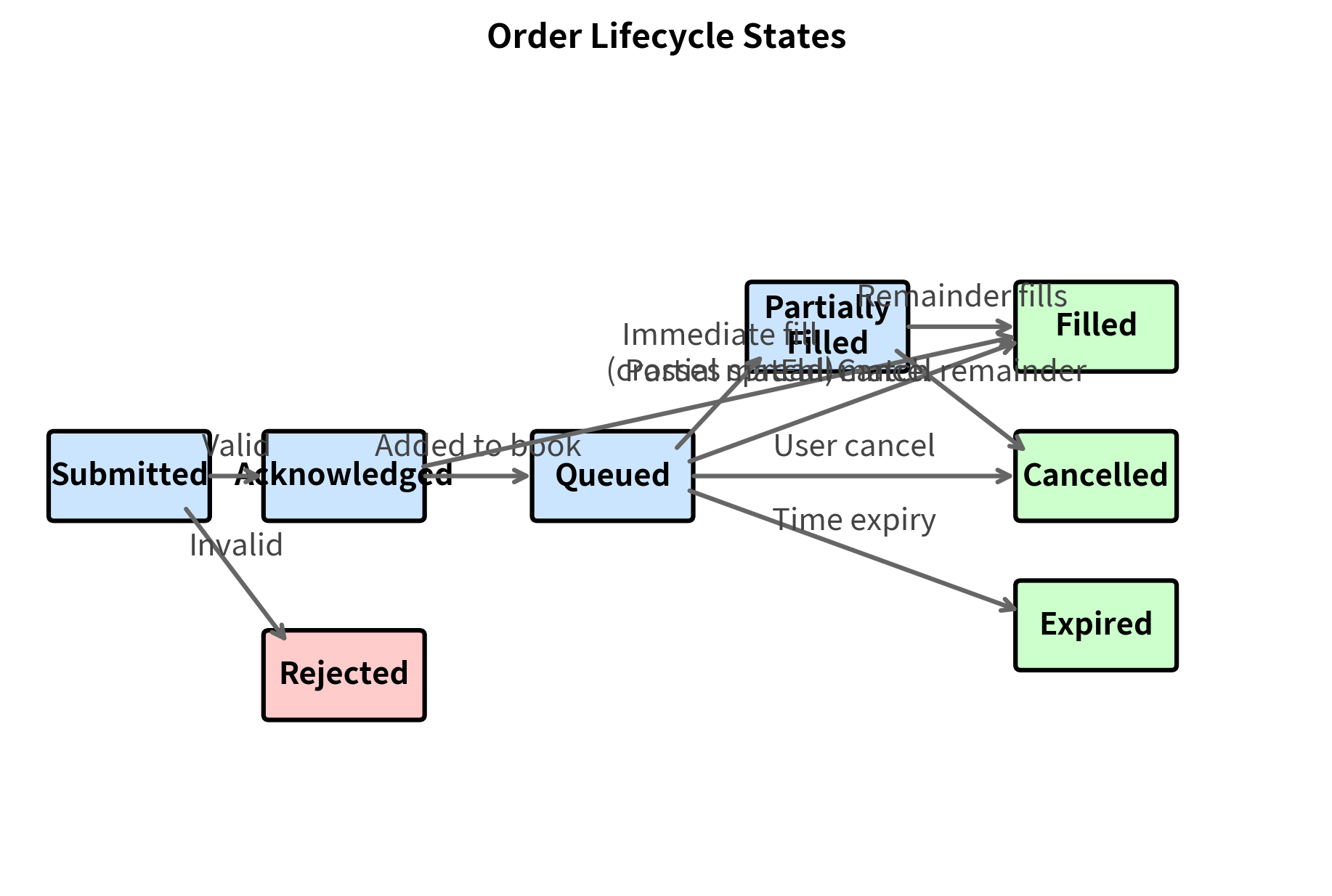
Understanding the order lifecycle is essential for building robust trading systems. Your system must handle each state transition, including partial fills that may occur over extended periods and unexpected rejections due to risk checks or connectivity issues.

Advanced Order TypesLink Copied

Beyond basic market and limit orders, exchanges and brokers offer specialized order types designed for specific trading needs.

Immediate-or-Cancel (IOC)Link Copied

An IOC order executes whatever quantity is immediately available and cancels the remainder. If you submit an IOC buy for 1,000 shares and only 400 are available at your limit price, you receive 400 shares and the remaining 600-share request is cancelled.

IOC orders are useful when you want to take available liquidity without leaving a footprint in the order book.

Fill-or-Kill (FOK)Link Copied

A FOK order must execute in its entirety immediately, or it is cancelled completely. Unlike IOC, there are no partial fills. This is used when partial execution would be undesirable, such as when hedging an exact position size.

Good-Till-Cancelled (GTC)Link Copied

Most orders are day orders; they expire at market close if unfilled. A GTC order remains active until it executes or is explicitly cancelled, potentially staying on the books for weeks or months.

Iceberg Orders (Reserve Orders)Link Copied

You might face a dilemma when executing large orders: you need to execute substantial orders, but displaying your full size would reveal your intentions and move prices against you. Iceberg orders solve this problem by splitting the order into a visible portion and a hidden reserve.

Iceberg Order

An iceberg order displays only a portion of the total order quantity in the visible order book. As the visible portion executes, more quantity is automatically revealed from the hidden reserve.

Iceberg orders help you minimize market impact by hiding the true size of your interest:

In[17]:

Code

@dataclass
class IcebergOrder:
    """An iceberg order with visible and hidden components."""

    total_quantity: int
    display_quantity: int
    price: float
    side: Side
    filled_quantity: int = 0

    @property
    def visible_quantity(self) -> int:
        remaining = self.total_quantity - self.filled_quantity
        return min(self.display_quantity, remaining)

    @property
    def hidden_quantity(self) -> int:
        return max(
            0,
            self.total_quantity - self.filled_quantity - self.display_quantity,
        )

    def fill(self, quantity: int) -> int:
        """Process a fill. Returns actual filled quantity."""
        fillable = min(quantity, self.total_quantity - self.filled_quantity)
        self.filled_quantity += fillable
        return fillable


# Example iceberg order
iceberg = IcebergOrder(
    total_quantity=10000, display_quantity=500, price=100.00, side=Side.BID
)

# Capture initial state
initial_visible = iceberg.visible_quantity
initial_hidden = iceberg.hidden_quantity

# Simulate execution: 3 fills of 500 shares
fill_size = 500
fills_count = 3
for _ in range(fills_count):
    iceberg.fill(fill_size)

# Capture final state
final_filled = iceberg.filled_quantity
final_visible = iceberg.visible_quantity
final_hidden = iceberg.hidden_quantity

@dataclass
class IcebergOrder:
    """An iceberg order with visible and hidden components."""

    total_quantity: int
    display_quantity: int
    price: float
    side: Side
    filled_quantity: int = 0

    @property
    def visible_quantity(self) -> int:
        remaining = self.total_quantity - self.filled_quantity
        return min(self.display_quantity, remaining)

    @property
    def hidden_quantity(self) -> int:
        return max(
            0,
            self.total_quantity - self.filled_quantity - self.display_quantity,
        )

    def fill(self, quantity: int) -> int:
        """Process a fill. Returns actual filled quantity."""
        fillable = min(quantity, self.total_quantity - self.filled_quantity)
        self.filled_quantity += fillable
        return fillable


# Example iceberg order
iceberg = IcebergOrder(
    total_quantity=10000, display_quantity=500, price=100.00, side=Side.BID
)

# Capture initial state
initial_visible = iceberg.visible_quantity
initial_hidden = iceberg.hidden_quantity

# Simulate execution: 3 fills of 500 shares
fill_size = 500
fills_count = 3
for _ in range(fills_count):
    iceberg.fill(fill_size)

# Capture final state
final_filled = iceberg.filled_quantity
final_visible = iceberg.visible_quantity
final_hidden = iceberg.hidden_quantity

Out[18]:

Console

Iceberg Order Example
========================================
Total Size: 10,000 shares
Display Size: 500 shares

What market participants see in order book:
  Bid: 500 shares @ $100.00

Actual state:
  Visible: 500 shares
  Hidden: 9,500 shares

After 3 fills of 500 shares each:
  Filled: 1,500 shares
  Visible: 500 shares
  Hidden: 8,000 shares

We look for 'iceberg detection' patterns repeated fills at the same price level that keep replenishing suggest hidden liquidity.

Key ParametersLink Copied

The key parameters for Iceberg Orders are:

Total Quantity: The full size of the order to be executed. This represents your complete trading interest.
Display Quantity: The portion of the order visible in the order book at any given time. This should be set large enough to attract counterparties but small enough to avoid revealing the true order size.
Hidden Quantity: The remaining quantity kept off the book, calculated as the difference between total quantity and display quantity. This hidden portion automatically replenishes the visible portion as fills occur.
Price: The limit price at which the order is placed. The entire order, both visible and hidden portions, executes only at this price or better.

Pegged OrdersLink Copied

Pegged orders automatically adjust their price relative to a reference point such as the NBBO (National Best Bid/Offer), midpoint, or a benchmark.

The main types of pegged orders include:

Primary peg: Pegged to the same-side NBBO (bid for buy orders, ask for sell orders)
Midpoint peg: Pegged to the midpoint between bid and ask
Market peg: Pegged to the opposite-side NBBO

Midpoint-pegged orders are popular for passive execution strategies because they potentially receive price improvement (better than the visible bid or ask) while still participating when the spread moves.

Algorithmic Order TypesLink Copied

Many brokers offer high-level algorithmic order types that translate into sophisticated execution strategies:

VWAP (Volume-Weighted Average Price): Execute throughout the day to match the market's volume pattern, targeting the volume-weighted average price
TWAP (Time-Weighted Average Price): Execute evenly over a specified time period
Percentage of Volume (POV): Execute as a target percentage of market volume
Implementation Shortfall: Minimize the difference between decision price and execution price

As we discussed in the chapter on transaction costs, these algorithms balance the trade-off between market impact and timing risk. We'll explore their implementation in detail in the next chapter on execution algorithms.

Bid-Ask Spread and LiquidityLink Copied

The bid-ask spread is perhaps the most fundamental indicator of market liquidity. It represents the cost of immediacy: the price you pay for instant execution versus patient limit orders.

Components of the SpreadLink Copied

Why does the spread exist at all? Why don't market makers simply quote the same price on both sides? The answer lies in the risks and costs that market makers face. They must be compensated for maintaining operations, holding inventory that may lose value, and trading against participants who possess superior information. The spread serves as this compensation.

The bid-ask spread compensates market makers for several costs and risks:

Order processing costs: The fixed costs of maintaining market-making operations
Inventory risk: The risk that prices move against the market maker's accumulated position
Adverse selection: The risk of trading against informed traders who have superior information

Mathematically, we can decompose the total spread $S$ into these three components:

S = C_{\text{proc}} + C_{\text{inv}} + C_{\text{adv}}

This decomposition provides insight into why spreads vary across different securities and market conditions. Let us examine each component:

$S$ : total bid-ask spread, the observable difference between the best ask and best bid prices
$C_{\text{proc}}$ : order processing component (fixed costs). This includes the infrastructure costs of running a trading operation: technology, connectivity, regulatory compliance, and personnel. For highly automated market makers, this component is relatively small and stable.
$C_{\text{inv}}$ : inventory risk component, proportional to volatility and position size. When a market maker buys shares from a seller, they hold inventory that may decline in value before they can sell it. Higher volatility increases this risk, requiring wider spreads as compensation.
$C_{\text{adv}}$ : adverse selection component, reflecting the probability of trading against better-informed participants. If some traders have superior information about future prices, the market maker loses money on average when trading with them. To break even, the market maker must recover these losses from uninformed traders through wider spreads.

In[19]:

Code

def decompose_spread_simple(
    spread: float, volatility: float, volume: float, tick_size: float
) -> dict:
    """
    Simplified spread decomposition model.
    Based on Huang and Stoll (1997) approach.
    """
    # Minimum spread is the tick size
    min_spread = tick_size

    # Adverse selection component increases with information asymmetry
    # Proxy: higher for volatile, lower-volume stocks
    adverse_selection = spread * 0.4  # typically 30-50% of spread

    # Inventory component increases with volatility
    inventory = spread * 0.3 * (volatility / 0.02)  # scaled by typical vol

    # Order processing is the residual
    order_processing = max(min_spread, spread - adverse_selection - inventory)

    return {
        "total_spread": spread,
        "adverse_selection": adverse_selection,
        "inventory": inventory,
        "order_processing": order_processing,
    }


# Example for different stocks
stocks = [
    {
        "name": "Large Cap Tech",
        "spread": 0.01,
        "vol": 0.25,
        "volume": 10_000_000,
    },
    {
        "name": "Mid Cap Industrial",
        "spread": 0.05,
        "vol": 0.30,
        "volume": 500_000,
    },
    {
        "name": "Small Cap Biotech",
        "spread": 0.15,
        "vol": 0.50,
        "volume": 100_000,
    },
]

# Calculate decompositions
decompositions = []
tick_size = 0.01
for stock in stocks:
    decomp = decompose_spread_simple(
        stock["spread"], stock["vol"], stock["volume"], tick_size
    )
    decompositions.append((stock, decomp))

def decompose_spread_simple(
    spread: float, volatility: float, volume: float, tick_size: float
) -> dict:
    """
    Simplified spread decomposition model.
    Based on Huang and Stoll (1997) approach.
    """
    # Minimum spread is the tick size
    min_spread = tick_size

    # Adverse selection component increases with information asymmetry
    # Proxy: higher for volatile, lower-volume stocks
    adverse_selection = spread * 0.4  # typically 30-50% of spread

    # Inventory component increases with volatility
    inventory = spread * 0.3 * (volatility / 0.02)  # scaled by typical vol

    # Order processing is the residual
    order_processing = max(min_spread, spread - adverse_selection - inventory)

    return {
        "total_spread": spread,
        "adverse_selection": adverse_selection,
        "inventory": inventory,
        "order_processing": order_processing,
    }


# Example for different stocks
stocks = [
    {
        "name": "Large Cap Tech",
        "spread": 0.01,
        "vol": 0.25,
        "volume": 10_000_000,
    },
    {
        "name": "Mid Cap Industrial",
        "spread": 0.05,
        "vol": 0.30,
        "volume": 500_000,
    },
    {
        "name": "Small Cap Biotech",
        "spread": 0.15,
        "vol": 0.50,
        "volume": 100_000,
    },
]

# Calculate decompositions
decompositions = []
tick_size = 0.01
for stock in stocks:
    decomp = decompose_spread_simple(
        stock["spread"], stock["vol"], stock["volume"], tick_size
    )
    decompositions.append((stock, decomp))

Out[20]:

Console

Spread Decomposition by Stock Type
============================================================

Large Cap Tech
  Total Spread: $0.010
  Adverse Selection: $0.004 (40%)
  Inventory Risk: $0.037 (375%)
  Order Processing: $0.010 (100%)

Mid Cap Industrial
  Total Spread: $0.050
  Adverse Selection: $0.020 (40%)
  Inventory Risk: $0.225 (450%)
  Order Processing: $0.010 (20%)

Small Cap Biotech
  Total Spread: $0.150
  Adverse Selection: $0.060 (40%)
  Inventory Risk: $1.125 (750%)
  Order Processing: $0.010 (7%)

The results illustrate how market characteristics drive spread composition. For the Small Cap Biotech stock, adverse selection and inventory risks constitute a much larger portion of the spread compared to the Large Cap Tech stock, reflecting higher volatility and lower liquidity.

The adverse selection component is particularly important for you. When you have better information than the market, you benefit from the adverse selection cost that market makers embed in spreads. Conversely, when you're trading without an edge, you're paying this cost to informed traders.

Key ParametersLink Copied

The key parameters for the spread decomposition model are:

spread: The observed bid-ask spread in the market. This is the starting point for decomposition and represents the total cost of crossing from bid to ask.
volatility: The volatility of the asset, which increases inventory risk. Higher volatility means greater potential for adverse price movements while the market maker holds inventory.
volume: Trading volume, used here as a proxy for liquidity and adverse selection risk. Higher volume typically correlates with lower adverse selection since uninformed traders constitute a larger share of the flow.
tick_size: The minimum price increment, acting as a lower bound for the spread. Regulatory requirements and exchange rules establish this minimum, which constrains how narrow spreads can become even for the most liquid securities.

Order Book Depth and LiquidityLink Copied

Beyond the spread, the depth of the order book at various price levels indicates how much liquidity is available before prices move:

In[21]:

Code

def calculate_liquidity_metrics(book: OrderBook, max_levels: int = 10) -> dict:
    """Calculate various liquidity metrics from an order book."""
    bid_levels, ask_levels = book.get_book_snapshot(max_levels)

    # Depth at best prices
    best_bid_depth = bid_levels[0][1] if bid_levels else 0
    best_ask_depth = ask_levels[0][1] if ask_levels else 0

    # Total visible depth
    total_bid_depth = sum(qty for _, qty in bid_levels)
    total_ask_depth = sum(qty for _, qty in ask_levels)

    # Book imbalance
    total_depth = total_bid_depth + total_ask_depth
    imbalance = (
        (total_bid_depth - total_ask_depth) / total_depth
        if total_depth > 0
        else 0
    )

    # Depth-weighted spread
    spread = book.get_spread()
    weighted_spread = (
        spread * (best_bid_depth + best_ask_depth) if spread else 0
    )

    return {
        "spread": spread,
        "best_bid_depth": best_bid_depth,
        "best_ask_depth": best_ask_depth,
        "total_bid_depth": total_bid_depth,
        "total_ask_depth": total_ask_depth,
        "book_imbalance": imbalance,
        "midprice": book.get_midprice(),
    }


# Create a more realistic order book
np.random.seed(123)
realistic_book = OrderBook("AAPL")

# Build with realistic depth profile (more at worse prices)
for i, price in enumerate([199.95, 199.90, 199.85, 199.80, 199.75]):
    depth = int(np.random.normal(1000 + i * 500, 200))
    for _ in range(np.random.randint(3, 8)):
        realistic_book.add_limit_order(Side.BID, price, depth // 5)

for i, price in enumerate([200.00, 200.05, 200.10, 200.15, 200.20]):
    depth = int(np.random.normal(1000 + i * 500, 200))
    for _ in range(np.random.randint(3, 8)):
        realistic_book.add_limit_order(Side.ASK, price, depth // 5)

metrics = calculate_liquidity_metrics(realistic_book)

def calculate_liquidity_metrics(book: OrderBook, max_levels: int = 10) -> dict:
    """Calculate various liquidity metrics from an order book."""
    bid_levels, ask_levels = book.get_book_snapshot(max_levels)

    # Depth at best prices
    best_bid_depth = bid_levels[0][1] if bid_levels else 0
    best_ask_depth = ask_levels[0][1] if ask_levels else 0

    # Total visible depth
    total_bid_depth = sum(qty for _, qty in bid_levels)
    total_ask_depth = sum(qty for _, qty in ask_levels)

    # Book imbalance
    total_depth = total_bid_depth + total_ask_depth
    imbalance = (
        (total_bid_depth - total_ask_depth) / total_depth
        if total_depth > 0
        else 0
    )

    # Depth-weighted spread
    spread = book.get_spread()
    weighted_spread = (
        spread * (best_bid_depth + best_ask_depth) if spread else 0
    )

    return {
        "spread": spread,
        "best_bid_depth": best_bid_depth,
        "best_ask_depth": best_ask_depth,
        "total_bid_depth": total_bid_depth,
        "total_ask_depth": total_ask_depth,
        "book_imbalance": imbalance,
        "midprice": book.get_midprice(),
    }


# Create a more realistic order book
np.random.seed(123)
realistic_book = OrderBook("AAPL")

# Build with realistic depth profile (more at worse prices)
for i, price in enumerate([199.95, 199.90, 199.85, 199.80, 199.75]):
    depth = int(np.random.normal(1000 + i * 500, 200))
    for _ in range(np.random.randint(3, 8)):
        realistic_book.add_limit_order(Side.BID, price, depth // 5)

for i, price in enumerate([200.00, 200.05, 200.10, 200.15, 200.20]):
    depth = int(np.random.normal(1000 + i * 500, 200))
    for _ in range(np.random.randint(3, 8)):
        realistic_book.add_limit_order(Side.ASK, price, depth // 5)

metrics = calculate_liquidity_metrics(realistic_book)

Out[22]:

Console

Order Book Liquidity Metrics
=============================================
Midprice: $199.97
Spread: $0.05 (2.5 bps)

Depth Analysis:
  Best Bid Depth: 1,092 shares
  Best Ask Depth: 728 shares
  Total Bid Depth (5 levels): 9,171 shares
  Total Ask Depth (5 levels): 9,438 shares

Book Imbalance: -1.43%

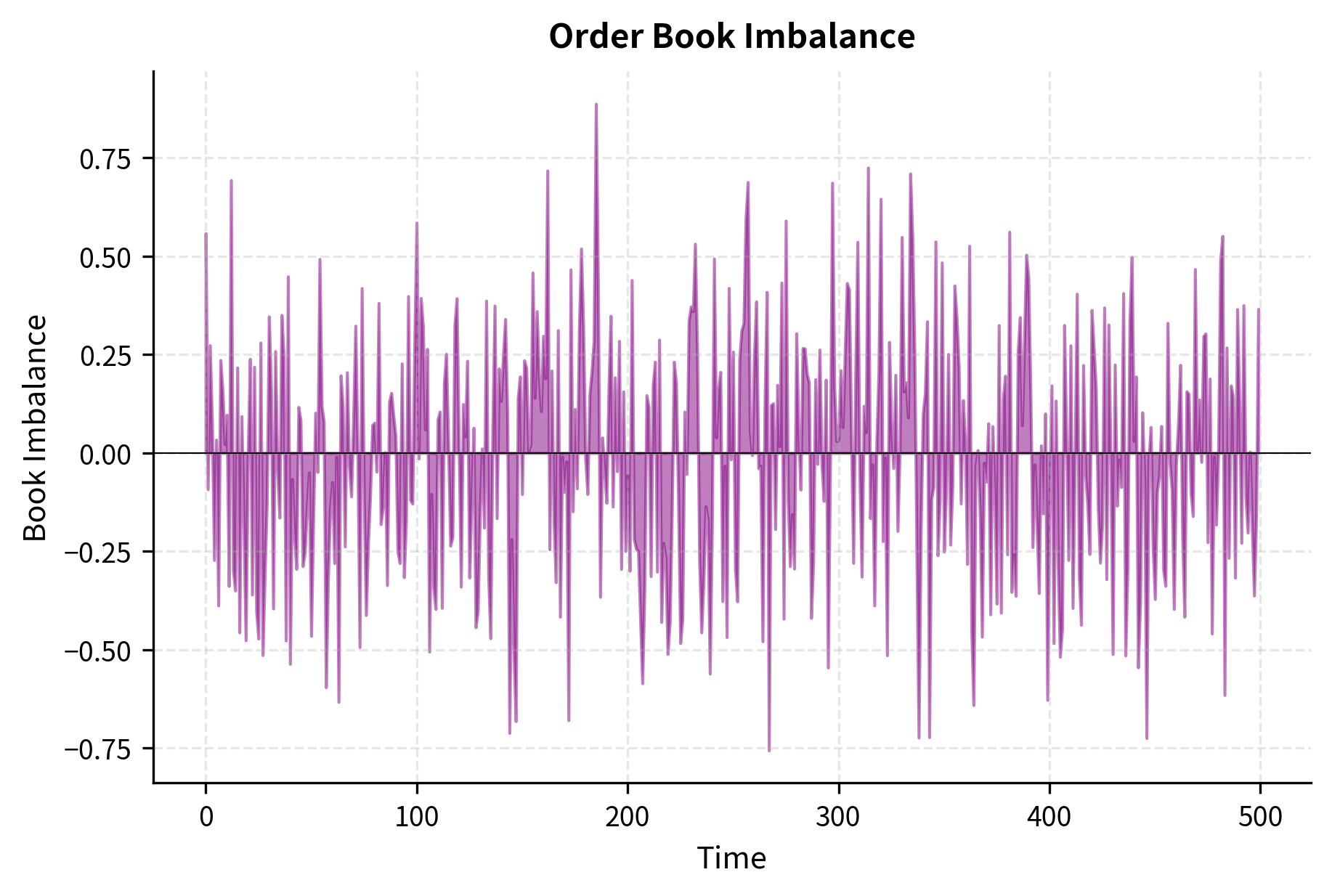
Book imbalance (or Order Book Imbalance, OBI) is a commonly studied signal in market microstructure research. The positive imbalance calculated above indicates stronger buying pressure in our simulated book, as bid volume exceeds ask volume. This metric quantifies the disparity between buying and selling pressure in the order book and can be expressed mathematically as:

\rho = \frac{V_b - V_a}{V_b + V_a}

Understanding this formula requires examining what each term represents and why the specific mathematical form was chosen:

$\rho$ : order book imbalance, ranging from -1 to +1. The Greek letter rho is commonly used to denote this imbalance measure. A value of +1 would indicate all visible liquidity is on the bid side (maximum buying pressure), while -1 indicates all liquidity is on the ask side (maximum selling pressure). A value of zero indicates perfect balance.
$V_b$ : total volume at the best bid (or top $N$ levels). This measures the depth of buying interest in the market. Larger values suggest substantial demand at current prices.
$V_a$ : total volume at the best ask (or top $N$ levels). This measures the depth of selling interest. Larger values suggest substantial supply at current prices.

The formula uses a normalized difference (dividing by the sum) rather than a simple difference because this produces a bounded measure that is comparable across securities with different typical order sizes. A stock with 10,000 shares on the bid and 8,000 on the ask has the same imbalance as a stock with 100 shares on the bid and 80 on the ask: both have $\rho = 0.11$ .

A positive $\rho$ indicates stronger buying pressure (more bids), while a negative value suggests selling pressure. Empirically, order book imbalance tends to predict short-term price movements: an excess of bids relative to asks often precedes price increases.

Dark Pools and Hidden LiquidityLink Copied

Not all liquidity is visible in the public order book. Dark pools are private trading venues that match orders without displaying quotes publicly.

Why Dark Pools ExistLink Copied

Dark pools emerged to address a fundamental tension: you might want to execute size without revealing your intentions to the market. When you need to sell $500 million of stock announcing that size would move prices against you before you can execute.

The key features of dark pools include:

Pre-trade anonymity: Order sizes and prices are not displayed publicly
Reduced information leakage: Other traders can't see your intentions
Potential price improvement: Many dark pools match at the midpoint, providing better prices than the lit market
Delayed reporting: Trades may not be reported until after execution

Dark pools now represent a substantial portion of U.S. equity volume:

Out[23]:

Visualization

Pie chart showing trading volume distribution: exchanges, dark pools, and other venues. — Approximate distribution of U.S. equity trading volume across different venue types. Off-exchange venues, including dark pools and wholesalers, account for over 50% of volume, illustrating the fragmentation of modern liquidity.

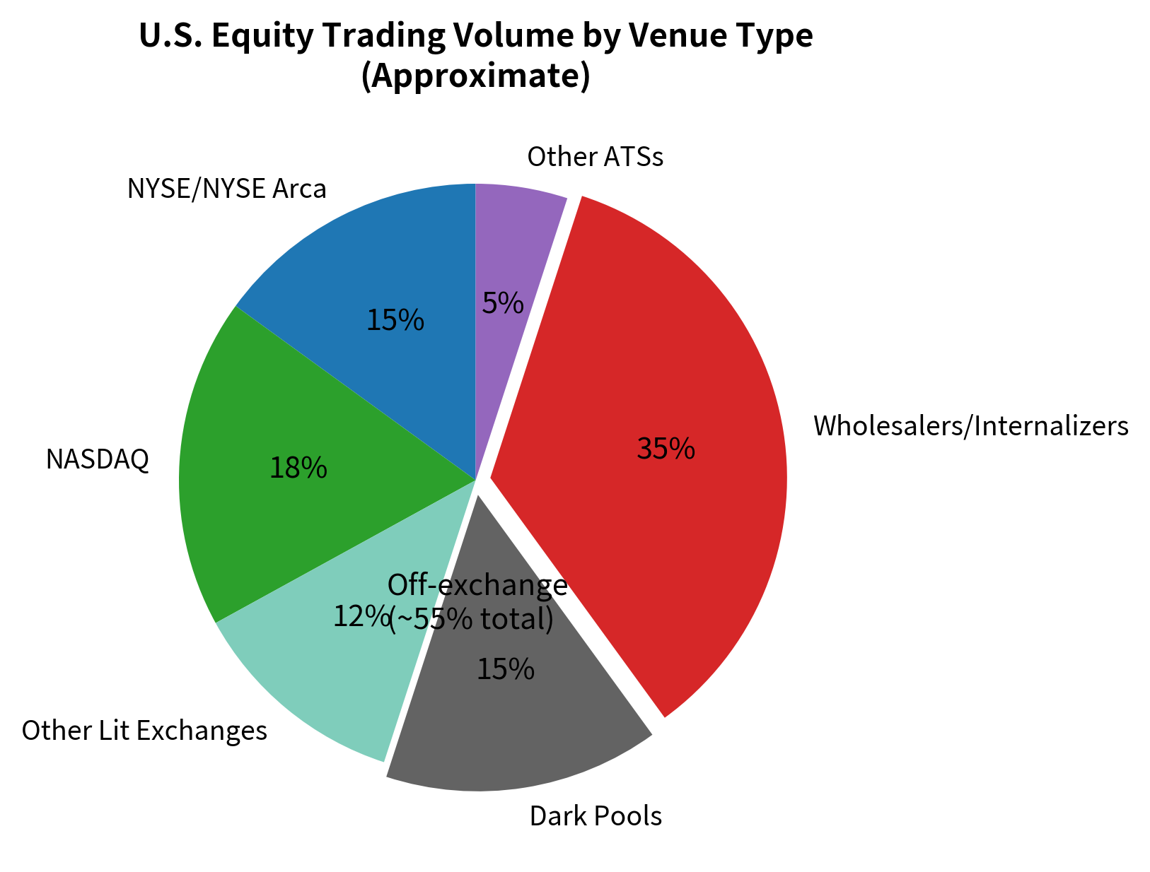
The significant share of off-exchange trading has important implications for order book analysis: the visible lit order book represents only part of the available liquidity. This is why execution algorithms often send orders to multiple venues, including dark pools, to access hidden liquidity.

Types of Dark Pool ParticipantsLink Copied

Understanding who participates in dark pools helps assess their utility:

Block-crossing networks: Match large institutional orders, often at scheduled intervals
Continuous dark pools: Match orders in real-time, similar to exchanges but without displayed quotes
Broker-dealer internalization: Brokers fill customer orders against their own inventory
Exchange dark order types: Even lit exchanges offer hidden order types

Risks of Dark Pool TradingLink Copied

While dark pools offer benefits, they also carry risks:

Adverse selection: Informed traders may selectively route to dark pools when beneficial to them
Information leakage: Some dark pools have been found to expose order information to select participants
Fill rate uncertainty: You may get partial or no fills, requiring lit market backup
Gaming: Predatory traders may probe dark pools for hidden orders

Order Book Dynamics and Price ImpactLink Copied

The order book is not static; it evolves continuously as orders arrive, execute, and cancel. Understanding these dynamics is crucial for execution and short-term trading strategies.

Event-Driven Order Book UpdatesLink Copied

Order book changes occur through several events:

In[24]:

Code

class OrderBookEvent:
    """Base class for order book events."""

    pass


@dataclass
class NewOrder(OrderBookEvent):
    order: Order


@dataclass
class CancelOrder(OrderBookEvent):
    order_id: int


@dataclass
class Trade(OrderBookEvent):
    price: float
    quantity: int
    aggressor_side: Side  # which side initiated the trade


def simulate_order_book_dynamics(
    book: OrderBook, n_events: int = 100
) -> List[dict]:
    """Simulate order book dynamics and track midprice evolution."""
    np.random.seed(42)

    history = []
    midprice = book.get_midprice()

    for t in range(n_events):
        # Record state before event
        mid_before = book.get_midprice()
        spread_before = book.get_spread()

        # Generate random event
        event_type = np.random.choice(
            [
                "new_bid",
                "new_ask",
                "cancel_bid",
                "cancel_ask",
                "market_buy",
                "market_sell",
            ],
            p=[0.25, 0.25, 0.15, 0.15, 0.10, 0.10],
        )

        if event_type == "new_bid":
            price = midprice - np.random.exponential(0.02)
            qty = np.random.randint(100, 500)
            book.add_limit_order(Side.BID, round(price, 2), qty)

        elif event_type == "new_ask":
            price = midprice + np.random.exponential(0.02)
            qty = np.random.randint(100, 500)
            book.add_limit_order(Side.ASK, round(price, 2), qty)

        elif event_type in ["market_buy", "market_sell"]:
            side = Side.BID if event_type == "market_buy" else Side.ASK
            qty = np.random.randint(200, 800)
            execute_market_order(book, side, qty)

        # Skip cancel events for simplicity in this simulation

        # Record state after event
        mid_after = book.get_midprice()
        spread_after = book.get_spread()

        if mid_after is not None:
            midprice = mid_after
            history.append(
                {
                    "time": t,
                    "event": event_type,
                    "midprice": mid_after,
                    "spread": spread_after,
                    "midprice_change": (mid_after - mid_before)
                    if mid_before
                    else 0,
                }
            )

    return history

class OrderBookEvent:
    """Base class for order book events."""

    pass


@dataclass
class NewOrder(OrderBookEvent):
    order: Order


@dataclass
class CancelOrder(OrderBookEvent):
    order_id: int


@dataclass
class Trade(OrderBookEvent):
    price: float
    quantity: int
    aggressor_side: Side  # which side initiated the trade


def simulate_order_book_dynamics(
    book: OrderBook, n_events: int = 100
) -> List[dict]:
    """Simulate order book dynamics and track midprice evolution."""
    np.random.seed(42)

    history = []
    midprice = book.get_midprice()

    for t in range(n_events):
        # Record state before event
        mid_before = book.get_midprice()
        spread_before = book.get_spread()

        # Generate random event
        event_type = np.random.choice(
            [
                "new_bid",
                "new_ask",
                "cancel_bid",
                "cancel_ask",
                "market_buy",
                "market_sell",
            ],
            p=[0.25, 0.25, 0.15, 0.15, 0.10, 0.10],
        )

        if event_type == "new_bid":
            price = midprice - np.random.exponential(0.02)
            qty = np.random.randint(100, 500)
            book.add_limit_order(Side.BID, round(price, 2), qty)

        elif event_type == "new_ask":
            price = midprice + np.random.exponential(0.02)
            qty = np.random.randint(100, 500)
            book.add_limit_order(Side.ASK, round(price, 2), qty)

        elif event_type in ["market_buy", "market_sell"]:
            side = Side.BID if event_type == "market_buy" else Side.ASK
            qty = np.random.randint(200, 800)
            execute_market_order(book, side, qty)

        # Skip cancel events for simplicity in this simulation

        # Record state after event
        mid_after = book.get_midprice()
        spread_after = book.get_spread()

        if mid_after is not None:
            midprice = mid_after
            history.append(
                {
                    "time": t,
                    "event": event_type,
                    "midprice": mid_after,
                    "spread": spread_after,
                    "midprice_change": (mid_after - mid_before)
                    if mid_before
                    else 0,
                }
            )

    return history

In[25]:

Code

# Create fresh book and simulate
sim_book = OrderBook("XYZ")

# Initialize with some depth
for price in np.arange(99.70, 99.96, 0.01):
    for _ in range(3):
        sim_book.add_limit_order(
            Side.BID, round(price, 2), np.random.randint(200, 600)
        )

for price in np.arange(100.00, 100.26, 0.01):
    for _ in range(3):
        sim_book.add_limit_order(
            Side.ASK, round(price, 2), np.random.randint(200, 600)
        )

# Run simulation
history = simulate_order_book_dynamics(sim_book, n_events=200)
history_df = pd.DataFrame(history)

# Create fresh book and simulate
sim_book = OrderBook("XYZ")

# Initialize with some depth
for price in np.arange(99.70, 99.96, 0.01):
    for _ in range(3):
        sim_book.add_limit_order(
            Side.BID, round(price, 2), np.random.randint(200, 600)
        )

for price in np.arange(100.00, 100.26, 0.01):
    for _ in range(3):
        sim_book.add_limit_order(
            Side.ASK, round(price, 2), np.random.randint(200, 600)
        )

# Run simulation
history = simulate_order_book_dynamics(sim_book, n_events=200)
history_df = pd.DataFrame(history)

Out[26]:

Visualization

Simulated midprice evolution over 200 events showing the impact of market orders. Vertical lines indicate buy (green) and sell (red) market orders that consume liquidity, often causing immediate shifts in the midprice.

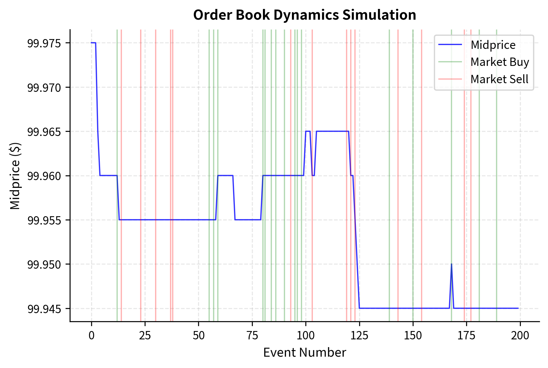
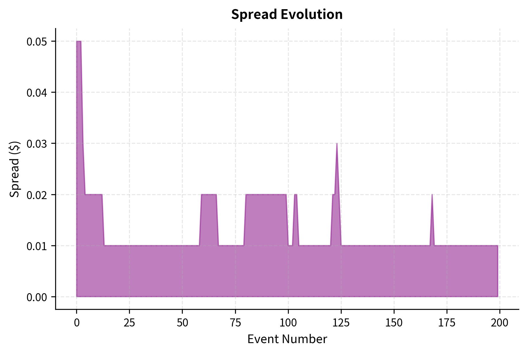
The simulation reveals several realistic patterns. Market orders cause immediate price impact (green and red vertical lines correspond to market buys and sells). The spread widens when liquidity is consumed and gradually tightens as new limit orders arrive.

Order Flow Imbalance and Price PredictionLink Copied

Research in market microstructure has established that order flow imbalance (the difference between buy and sell volume) predicts short-term price movements. The intuition behind this relationship is straightforward: when more buyers than sellers are actively trading, prices tend to rise to attract additional sellers, and vice versa.

We can define the Order Flow Imbalance (OFI) over a time window as:

\text{OFI} = \sum_{i=1}^{N} q_i \cdot d_i

This formula captures the net directional pressure from actual trades. Let us understand each component:

$\text{OFI}$ : Order Flow Imbalance over the time window. This is a signed quantity: positive values indicate net buying pressure, negative values indicate net selling pressure.
$q_i$ : quantity of the $i$ -th trade. Larger trades contribute more to the imbalance, reflecting the greater information content and market impact of size.
$d_i$ : direction of the trade (+1 for buyer-initiated, -1 for seller-initiated). A buyer-initiated trade occurs when a buyer submits a market order that executes against resting limit sell orders. A seller-initiated trade occurs when a seller's market order executes against resting limit buy orders.
$N$ : number of trades in the window. The window choice affects signal characteristics: shorter windows capture high-frequency dynamics, while longer windows smooth out noise but may lag actual price movements.

This relationship forms the basis for many high-frequency trading strategies, as we discussed in Part VI.

In[27]:

Code

def calculate_order_flow_imbalance(
    trades: pd.DataFrame, window: int = 10
) -> pd.Series:
    """
    Calculate order flow imbalance over a rolling window.
    Assumes trades dataframe has 'quantity' and 'aggressor_side' columns.
    """
    # Signed volume: positive for buys, negative for sells
    trades["signed_volume"] = np.where(
        trades["aggressor_side"] == "buy",
        trades["quantity"],
        -trades["quantity"],
    )

    # Rolling sum of signed volume
    rolling_signed = trades["signed_volume"].rolling(window=window).sum()
    rolling_total = trades["quantity"].abs().rolling(window=window).sum()

    imbalance = rolling_signed / rolling_total
    return imbalance


# Create synthetic trade data
np.random.seed(456)
n_trades = 500
synthetic_trades = pd.DataFrame(
    {
        "time": np.arange(n_trades),
        "price": 100 + np.cumsum(np.random.randn(n_trades) * 0.01),
        "quantity": np.random.randint(100, 1000, n_trades),
        "aggressor_side": np.random.choice(
            ["buy", "sell"], n_trades, p=[0.52, 0.48]
        ),
    }
)

# Calculate imbalance
synthetic_trades["imbalance"] = calculate_order_flow_imbalance(
    synthetic_trades, window=20
)

# Calculate future return
synthetic_trades["future_return"] = (
    synthetic_trades["price"].pct_change(5).shift(-5)
)

def calculate_order_flow_imbalance(
    trades: pd.DataFrame, window: int = 10
) -> pd.Series:
    """
    Calculate order flow imbalance over a rolling window.
    Assumes trades dataframe has 'quantity' and 'aggressor_side' columns.
    """
    # Signed volume: positive for buys, negative for sells
    trades["signed_volume"] = np.where(
        trades["aggressor_side"] == "buy",
        trades["quantity"],
        -trades["quantity"],
    )

    # Rolling sum of signed volume
    rolling_signed = trades["signed_volume"].rolling(window=window).sum()
    rolling_total = trades["quantity"].abs().rolling(window=window).sum()

    imbalance = rolling_signed / rolling_total
    return imbalance


# Create synthetic trade data
np.random.seed(456)
n_trades = 500
synthetic_trades = pd.DataFrame(
    {
        "time": np.arange(n_trades),
        "price": 100 + np.cumsum(np.random.randn(n_trades) * 0.01),
        "quantity": np.random.randint(100, 1000, n_trades),
        "aggressor_side": np.random.choice(
            ["buy", "sell"], n_trades, p=[0.52, 0.48]
        ),
    }
)

# Calculate imbalance
synthetic_trades["imbalance"] = calculate_order_flow_imbalance(
    synthetic_trades, window=20
)

# Calculate future return
synthetic_trades["future_return"] = (
    synthetic_trades["price"].pct_change(5).shift(-5)
)

In[28]:

Code

## Drop NaN values for analysis
analysis_df = synthetic_trades.dropna()

## Fit regression line
coef = np.polyfit(
    analysis_df["imbalance"], analysis_df["future_return"] * 100, 1
)
x_line = np.linspace(
    analysis_df["imbalance"].min(), analysis_df["imbalance"].max(), 100
)
y_line = coef[0] * x_line + coef[1]

## Drop NaN values for analysis
analysis_df = synthetic_trades.dropna()

## Fit regression line
coef = np.polyfit(
    analysis_df["imbalance"], analysis_df["future_return"] * 100, 1
)
x_line = np.linspace(
    analysis_df["imbalance"].min(), analysis_df["imbalance"].max(), 100
)
y_line = coef[0] * x_line + coef[1]

Out[29]:

Visualization

Scatter plot showing order flow imbalance on x-axis and 5-period future return on y-axis with regression line. — Scatter plot of order flow imbalance (OFI) versus 5-period future returns. The positive correlation (red regression line) demonstrates that periods of net buying pressure typically precede positive price returns, though with significant noise.

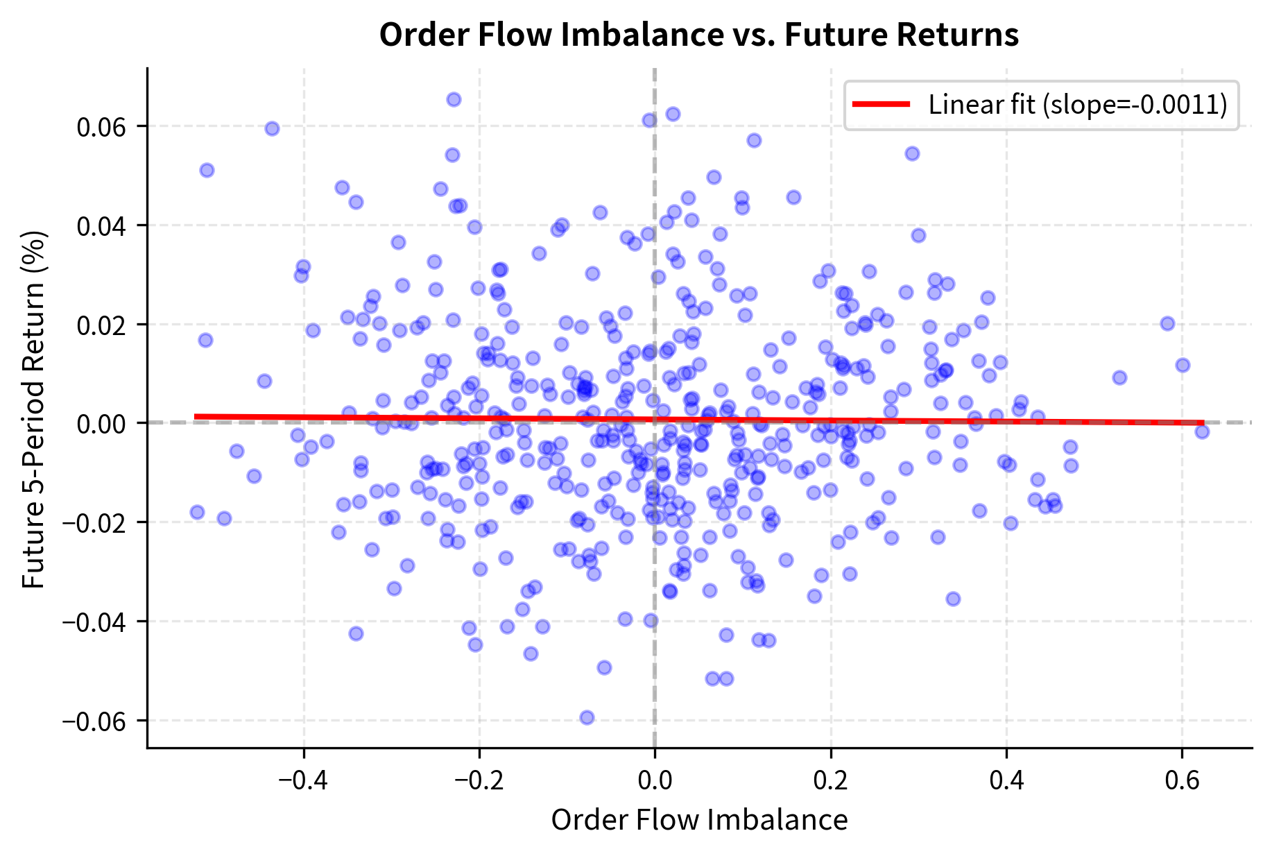
The positive slope indicates that order flow imbalance has predictive power for short-term returns. However, the relationship is noisy and exploiting it requires accounting for execution costs that may exceed the signal's value.

Market Manipulation and Regulatory ConsiderationsLink Copied

Understanding market microstructure also means recognizing when it can be exploited for manipulation. Several practices are illegal but worth knowing to recognize and avoid.

Spoofing and LayeringLink Copied

Spoofing

Spoofing is the practice of placing orders with the intent to cancel them before execution, in order to create a false impression of supply or demand and move prices.

A spoofer might place large visible bid orders to create the appearance of buying interest, causing prices to rise. They then sell into the artificially inflated price, cancel their bids, and profit from the price reversal. This practice is explicitly prohibited under the Dodd-Frank Act.

The mechanics work as follows:

Layering bids: Place multiple large limit buy orders below the current price
Perception manipulation: Other traders see apparent demand and buy, pushing prices up
Execute the real trade: Sell into the higher price on the opposite side
Cancel the layers: Remove the fake bids before they can execute

Detection algorithms look for patterns such as high order-to-trade ratios, rapid cancellations, and repetitive layering behavior.

Quote StuffingLink Copied

Quote stuffing involves submitting and canceling orders at extremely high rates to slow down exchange systems or create confusion. By overwhelming the market data feed, the manipulator may gain a latency advantage.

Wash TradingLink Copied

Wash trading occurs when the same entity is on both sides of a trade, creating the false appearance of trading activity. This inflates volume statistics and can manipulate benchmarks that depend on trading volume.

Front-RunningLink Copied

While not always illegal depending on the context, front-running involves trading ahead of known customer orders. If a broker knows a large customer buy order is coming, trading ahead to profit from the expected price impact is prohibited.

Modern execution algorithms are designed to minimize information leakage that could enable front-running by breaking up orders and randomizing execution patterns.

Practical Analysis: Level 2 DataLink Copied

Let's work through a practical example of analyzing Level 2 order book data, the type of data that you use to understand market microstructure in real-time.

In[30]:

Code

def generate_synthetic_l2_snapshots(
    n_snapshots: int = 100, levels: int = 5
) -> pd.DataFrame:
    """
    Generate synthetic Level 2 order book snapshots.
    Returns DataFrame with timestamp, bid/ask prices and sizes at each level.
    """
    np.random.seed(789)

    snapshots = []
    midprice = 100.0
    base_spread = 0.05

    for t in range(n_snapshots):
        # Random walk midprice
        midprice += np.random.randn() * 0.02

        # Time-varying spread (widens with volatility)
        spread = base_spread * (1 + 0.2 * np.abs(np.random.randn()))

        snapshot = {"timestamp": t}

        # Generate bid levels
        for i in range(levels):
            level_price = midprice - spread / 2 - i * 0.01
            level_size = int(np.random.exponential(500) * (1 + i * 0.3))
            snapshot[f"bid_price_{i + 1}"] = round(level_price, 2)
            snapshot[f"bid_size_{i + 1}"] = level_size

        # Generate ask levels
        for i in range(levels):
            level_price = midprice + spread / 2 + i * 0.01
            level_size = int(np.random.exponential(500) * (1 + i * 0.3))
            snapshot[f"ask_price_{i + 1}"] = round(level_price, 2)
            snapshot[f"ask_size_{i + 1}"] = level_size

        snapshots.append(snapshot)

    return pd.DataFrame(snapshots)


# Generate synthetic L2 data
l2_data = generate_synthetic_l2_snapshots(n_snapshots=500, levels=5)

def generate_synthetic_l2_snapshots(
    n_snapshots: int = 100, levels: int = 5
) -> pd.DataFrame:
    """
    Generate synthetic Level 2 order book snapshots.
    Returns DataFrame with timestamp, bid/ask prices and sizes at each level.
    """
    np.random.seed(789)

    snapshots = []
    midprice = 100.0
    base_spread = 0.05

    for t in range(n_snapshots):
        # Random walk midprice
        midprice += np.random.randn() * 0.02

        # Time-varying spread (widens with volatility)
        spread = base_spread * (1 + 0.2 * np.abs(np.random.randn()))

        snapshot = {"timestamp": t}

        # Generate bid levels
        for i in range(levels):
            level_price = midprice - spread / 2 - i * 0.01
            level_size = int(np.random.exponential(500) * (1 + i * 0.3))
            snapshot[f"bid_price_{i + 1}"] = round(level_price, 2)
            snapshot[f"bid_size_{i + 1}"] = level_size

        # Generate ask levels
        for i in range(levels):
            level_price = midprice + spread / 2 + i * 0.01
            level_size = int(np.random.exponential(500) * (1 + i * 0.3))
            snapshot[f"ask_price_{i + 1}"] = round(level_price, 2)
            snapshot[f"ask_size_{i + 1}"] = level_size

        snapshots.append(snapshot)

    return pd.DataFrame(snapshots)


# Generate synthetic L2 data
l2_data = generate_synthetic_l2_snapshots(n_snapshots=500, levels=5)

Now let's compute microstructure features from this data:

In[31]:

Code

def compute_microstructure_features(l2_df: pd.DataFrame) -> pd.DataFrame:
    """Compute various microstructure features from L2 data."""
    features = l2_df.copy()

    # Best bid and ask
    features["best_bid"] = features["bid_price_1"]
    features["best_ask"] = features["ask_price_1"]

    # Midprice and spread
    features["midprice"] = (features["best_bid"] + features["best_ask"]) / 2
    features["spread"] = features["best_ask"] - features["best_bid"]
    features["spread_bps"] = features["spread"] / features["midprice"] * 10000

    # Top of book imbalance
    features["tob_imbalance"] = (
        features["bid_size_1"] - features["ask_size_1"]
    ) / (features["bid_size_1"] + features["ask_size_1"])

    # Total depth at 5 levels
    bid_cols = [f"bid_size_{i}" for i in range(1, 6)]
    ask_cols = [f"ask_size_{i}" for i in range(1, 6)]
    features["total_bid_depth"] = features[bid_cols].sum(axis=1)
    features["total_ask_depth"] = features[ask_cols].sum(axis=1)

    # Full book imbalance
    features["book_imbalance"] = (
        features["total_bid_depth"] - features["total_ask_depth"]
    ) / (features["total_bid_depth"] + features["total_ask_depth"])

    # Volume-weighted bid/ask prices (proxy for depth-weighted prices)
    features["vwap_bid"] = (
        sum(
            features[f"bid_price_{i}"] * features[f"bid_size_{i}"]
            for i in range(1, 6)
        )
        / features["total_bid_depth"]
    )

    features["vwap_ask"] = (
        sum(
            features[f"ask_price_{i}"] * features[f"ask_size_{i}"]
            for i in range(1, 6)
        )
        / features["total_ask_depth"]
    )

    # Microprice (depth-weighted midprice)
    features["microprice"] = (
        features["best_bid"] * features["ask_size_1"]
        + features["best_ask"] * features["bid_size_1"]
    ) / (features["bid_size_1"] + features["ask_size_1"])

    return features


# Compute features
features_df = compute_microstructure_features(l2_data)

def compute_microstructure_features(l2_df: pd.DataFrame) -> pd.DataFrame:
    """Compute various microstructure features from L2 data."""
    features = l2_df.copy()

    # Best bid and ask
    features["best_bid"] = features["bid_price_1"]
    features["best_ask"] = features["ask_price_1"]

    # Midprice and spread
    features["midprice"] = (features["best_bid"] + features["best_ask"]) / 2
    features["spread"] = features["best_ask"] - features["best_bid"]
    features["spread_bps"] = features["spread"] / features["midprice"] * 10000

    # Top of book imbalance
    features["tob_imbalance"] = (
        features["bid_size_1"] - features["ask_size_1"]
    ) / (features["bid_size_1"] + features["ask_size_1"])

    # Total depth at 5 levels
    bid_cols = [f"bid_size_{i}" for i in range(1, 6)]
    ask_cols = [f"ask_size_{i}" for i in range(1, 6)]
    features["total_bid_depth"] = features[bid_cols].sum(axis=1)
    features["total_ask_depth"] = features[ask_cols].sum(axis=1)

    # Full book imbalance
    features["book_imbalance"] = (
        features["total_bid_depth"] - features["total_ask_depth"]
    ) / (features["total_bid_depth"] + features["total_ask_depth"])

    # Volume-weighted bid/ask prices (proxy for depth-weighted prices)
    features["vwap_bid"] = (
        sum(
            features[f"bid_price_{i}"] * features[f"bid_size_{i}"]
            for i in range(1, 6)
        )
        / features["total_bid_depth"]
    )

    features["vwap_ask"] = (
        sum(
            features[f"ask_price_{i}"] * features[f"ask_size_{i}"]
            for i in range(1, 6)
        )
        / features["total_ask_depth"]
    )

    # Microprice (depth-weighted midprice)
    features["microprice"] = (
        features["best_bid"] * features["ask_size_1"]
        + features["best_ask"] * features["bid_size_1"]
    ) / (features["bid_size_1"] + features["ask_size_1"])

    return features


# Compute features
features_df = compute_microstructure_features(l2_data)

Out[32]:

Console

Microstructure Feature Summary Statistics
=======================================================
       spread_bps  tob_imbalance  book_imbalance  total_bid_depth  total_ask_depth
count     500.000        500.000         500.000          500.000           500.00
mean        5.768         -0.005          -0.010         3995.422          4080.15
std         0.741          0.571           0.306         1830.485          1839.17
min         4.987         -1.000          -0.756          479.000           679.00
25%         5.006         -0.494          -0.249         2632.250          2812.75
50%         5.996         -0.020          -0.009         3683.500          3820.50
75%         6.010          0.487           0.211         5089.250          5122.75
max         8.020          0.988           0.887        11504.000         12962.00

The microprice is particularly interesting: it's a depth-weighted midprice that accounts for order book imbalance. Unlike the standard midprice which treats the bid and ask symmetrically, the microprice adjusts based on available liquidity. The intuition is that prices are more likely to move toward the side with less depth, since less volume is required to push the price in that direction.

We can derive the microprice formula by thinking about it as a weighted average where the weights are the opposite side's depth. When there is more depth on the bid side, the price is more likely to move upward (toward the ask), so we weight the ask price more heavily:

\begin{aligned} P_{\text{micro}} &= \frac{P_b V_a + P_a V_b}{V_b + V_a} && \text{(weighted average definition)} \\ &= P_a \left(\frac{V_b}{V_b + V_a}\right) + P_b \left(\frac{V_a}{V_b + V_a}\right) && \text{(rearrange terms)} \\ &= I \cdot P_a + (1-I) \cdot P_b && \text{(substitute imbalance ratio)} \end{aligned}

Let us examine each variable to understand the economic intuition:

$P_{\text{micro}}$ : microprice. This represents a more informed estimate of the security's fair value than the simple midprice. It incorporates order book depth information that may predict short-term price movements.
$P_b$ : best bid price. The highest price buyers are willing to pay.
$P_a$ : best ask price. The lowest price sellers are willing to accept.
$V_b$ : volume at the best bid. Represents the immediate buying liquidity. When this is large relative to the ask volume, it takes more selling to push the price down.
$V_a$ : volume at the best ask. Represents the immediate selling liquidity. When this is large relative to the bid volume, it takes more buying to push the price up.
$I$ : bid imbalance ratio, defined as $\frac{V_b}{V_b + V_a}$ . This ratio ranges from 0 to 1 and measures what fraction of top-of-book liquidity sits on the bid side.

When there's more depth on the bid side, the microprice shifts closer to the ask price, reflecting the likely direction of the next price move.

Out[33]:

Visualization

Comparison of the standard midprice (blue) and depth-weighted microprice (red) during the simulation. The microprice deviates from the midprice by accounting for order book depth, shifting toward the side with less liquidity to anticipate potential price moves.

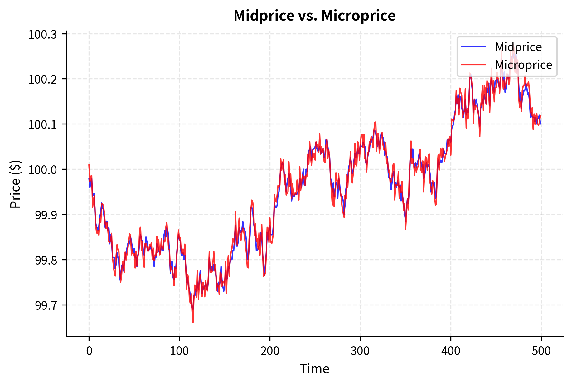
When book imbalance is positive (more bid depth), the microprice tends to be higher than the midprice, anticipating upward price pressure. This relationship forms the basis for many short-term trading signals.

Limitations and Practical ConsiderationsLink Copied

Market microstructure knowledge is essential but comes with important caveats for practical application.

The most fundamental limitation is the difference between simulation and reality. Our order book models assume clean, deterministic matching rules, but real markets involve multiple venues with different rules, hidden liquidity, latency, and occasional system glitches. A strategy that performs well in a simulated order book may fail in production due to factors that weren't modeled.

Latency creates an uneven playing field. The microstructure patterns we've discussed, such as order book imbalance and microprice signals, are actively exploited by high-frequency traders with sub-millisecond execution capabilities. By the time a retail or even institutional system observes these signals and acts, the opportunity may already be gone. The alpha in microstructure signals decays extremely rapidly, often within microseconds.

Data quality presents another challenge. Level 2 data is expensive, and historical order book data even more so. Reconstructing the order book from message data requires careful handling of order IDs, message sequencing, and exchange-specific quirks. Errors in data processing can create phantom signals or miss real ones.

The regulatory environment continues to evolve. Rules around dark pools, payment for order flow, market maker obligations, and algorithmic trading change regularly. Strategies that are profitable and legal today may become prohibited tomorrow, or new regulations may create opportunities that didn't exist before. The battle between regulators and manipulators is ongoing, with detection algorithms and manipulation techniques both becoming more sophisticated.

Finally, microstructure is inherently adversarial. Every informed trader's gain comes at someone else's expense, usually the market maker or other liquidity providers. As more participants use similar signals (like order book imbalance), the signals become crowded and less profitable. The market adapts, spreads tighten, and the bar for profitable microstructure trading keeps rising.

SummaryLink Copied

This chapter examined the mechanics of how modern electronic markets operate at the granular level. We covered the following key concepts:

Order Book Structure: The order book is the central mechanism for price discovery and trade execution. It consists of bid and ask levels, each with price and quantity information. The spread between best bid and best ask represents the cost of immediacy.

Order Types: Market orders provide execution certainty at the cost of price uncertainty. Limit orders provide price certainty at the cost of execution uncertainty. Advanced order types like iceberg orders, IOC, FOK, and pegged orders serve specialized needs.

Order Priority: Price-time priority (FIFO) is the dominant matching scheme for equities. Queue position matters: arriving earlier at a price level provides execution priority. Pro-rata matching, used in some markets, allocates fills proportionally to order size.

Spread Components: The bid-ask spread compensates market makers for order processing costs, inventory risk, and adverse selection. Understanding these components helps explain why spreads vary across securities.

Hidden Liquidity: Dark pools and hidden order types provide venues for executing large orders with reduced information leakage. Off-exchange trading represents a substantial portion of overall volume.

Order Book Dynamics: The order book evolves continuously through order arrivals, cancellations, and trades. Order flow imbalance provides short-term predictive signals, though exploiting them requires sophisticated infrastructure.

Market Manipulation: Spoofing, layering, quote stuffing, and wash trading are prohibited practices. Understanding them helps in recognition and avoidance, and informs the design of compliant systems.

The next chapter on execution algorithms builds directly on these concepts, translating microstructure knowledge into practical algorithms for optimal order execution.

QuizLink Copied

Test your understanding of market microstructure, order types, and liquidity dynamics with this interactive quiz.

Loading component...

Comments

Back to Quantitative Finance

Previous Chapter

High-Frequency Trading and Latency Arbitrage

Next Chapter

Optimal Execution Algorithms: TWAP, VWAP & Market Impact

Reference

BIBTEXAcademic

@misc{marketmicrostructureorderbooksexecutionmechanics, author = {Michael Brenndoerfer}, title = {Market Microstructure: Order Books & Execution Mechanics}, year = {2026}, url = {https://mbrenndoerfer.com/writing/market-microstructure-order-book-mechanics}, organization = {mbrenndoerfer.com}, note = {Accessed: 2025-01-01} }

APAAcademic

Michael Brenndoerfer (2026). Market Microstructure: Order Books & Execution Mechanics. Retrieved from https://mbrenndoerfer.com/writing/market-microstructure-order-book-mechanics

MLAAcademic

Michael Brenndoerfer. "Market Microstructure: Order Books & Execution Mechanics." 2026. Web. today. <https://mbrenndoerfer.com/writing/market-microstructure-order-book-mechanics>.

CHICAGOAcademic

Michael Brenndoerfer. "Market Microstructure: Order Books & Execution Mechanics." Accessed today. https://mbrenndoerfer.com/writing/market-microstructure-order-book-mechanics.

HARVARDAcademic

Michael Brenndoerfer (2026) 'Market Microstructure: Order Books & Execution Mechanics'. Available at: https://mbrenndoerfer.com/writing/market-microstructure-order-book-mechanics (Accessed: today).

SimpleBasic

Michael Brenndoerfer (2026). Market Microstructure: Order Books & Execution Mechanics. https://mbrenndoerfer.com/writing/market-microstructure-order-book-mechanics

Direct link:

https://mbrenndoerfer.com/writing/market-microstructure-order-book-mechanics

About the author: Michael Brenndoerfer

All opinions expressed here are my own and do not reflect the views of my employer.

Michael currently works as an Associate Director of Data Science at EQT Partners in Singapore, leading AI and data initiatives across private capital investments.

With over a decade of experience spanning private equity, management consulting, and software engineering, he specializes in building and scaling analytics capabilities from the ground up. He has published research in leading AI conferences and holds expertise in machine learning, natural language processing, and value creation through data.

View Full Resume Publications Contact Books

Market Microstructure: Order Books & Execution Mechanics

Market Microstructure and Order TypesLink Copied

The Order BookLink Copied

Structure of the Order BookLink Copied

Visualizing Order Book DepthLink Copied

Order TypesLink Copied

Market OrdersLink Copied

Limit OrdersLink Copied

Stop OrdersLink Copied

Stop-Limit ExampleLink Copied

Order Priority and MatchingLink Copied

Price-Time PriorityLink Copied

Pro-Rata MatchingLink Copied

Order LifecycleLink Copied

Advanced Order TypesLink Copied

Immediate-or-Cancel (IOC)Link Copied

Fill-or-Kill (FOK)Link Copied

Good-Till-Cancelled (GTC)Link Copied

Iceberg Orders (Reserve Orders)Link Copied

Key ParametersLink Copied

Pegged OrdersLink Copied

Algorithmic Order TypesLink Copied

Bid-Ask Spread and LiquidityLink Copied

Components of the SpreadLink Copied

Key ParametersLink Copied

Order Book Depth and LiquidityLink Copied

Dark Pools and Hidden LiquidityLink Copied

Why Dark Pools ExistLink Copied

Dark Pool Market ShareLink Copied

Types of Dark Pool ParticipantsLink Copied

Risks of Dark Pool TradingLink Copied

Order Book Dynamics and Price ImpactLink Copied

Event-Driven Order Book UpdatesLink Copied

Order Flow Imbalance and Price PredictionLink Copied

Market Manipulation and Regulatory ConsiderationsLink Copied

Spoofing and LayeringLink Copied

Quote StuffingLink Copied

Wash TradingLink Copied

Front-RunningLink Copied

Practical Analysis: Level 2 DataLink Copied

Limitations and Practical ConsiderationsLink Copied

SummaryLink Copied

QuizLink Copied

Comments

Reference

About the author: Michael Brenndoerfer

Related Content

High-Frequency Trading: Latency Arbitrage & Market Making

Market Making & Liquidity Provision: Optimal Quoting Models

Optimal Execution Algorithms: TWAP, VWAP & Market Impact

Stay updated

Comments

About the author: Michael Brenndoerfer

Related Content

High-Frequency Trading: Latency Arbitrage & Market Making

Market Making & Liquidity Provision: Optimal Quoting Models

Optimal Execution Algorithms: TWAP, VWAP & Market Impact

Stay updated