

Master transaction cost analysis and market impact modeling. Estimate spread, slippage, and liquidity to build realistic backtests and execution strategies.
Choose your expertise level to adjust how many terms are explained. Beginners see more tooltips, experts see fewer to maintain reading flow. Hover over underlined terms for instant definitions.
Transaction Costs and Market Impact
In the previous chapter on backtesting, we emphasized that a backtest is only as good as its assumptions. Transaction cost assumptions are critical and often underestimated. A strategy that appears highly profitable in a frictionless simulation can become unprofitable or even catastrophic when realistic trading costs are incorporated. This gap between theoretical and realized performance has destroyed countless strategies that looked promising on paper.
Transaction costs represent the difference between the price you expect to trade at and the price you actually achieve. They arise from multiple sources: explicit fees like commissions and taxes, implicit costs like bid-ask spreads, and market impact from your own trading activity. As a large institutional trader, you may find that market impact alone consumes a significant portion of expected alpha, particularly in less liquid markets or when executing large orders relative to available liquidity.
Modeling transaction costs is essential for strategy evaluation, position sizing, and execution. The relationship between trade size and cost is highly nonlinear: doubling your position size can more than double your transaction costs due to market impact effects. This has profound implications for strategy capacity and scalability.
This chapter develops a comprehensive framework for understanding, measuring, and incorporating transaction costs into quantitative trading systems. This chapter categorizes transaction costs, develops mathematical models for market impact, and integrates these models into strategy design and backtesting.
Types of Transaction Costs
Transaction costs can be decomposed into several distinct components, each with different characteristics and magnitudes depending on the market, instrument, and trading style. Understanding this decomposition is essential for accurate cost modeling. Each component behaves differently: some are fixed and predictable, others scale with trade size, and still others depend on market conditions at the moment of execution. By carefully separating these components, we can build more accurate models and identify which costs dominate in different trading scenarios.
Explicit Costs
Explicit costs are directly observable and contractually specified. They include:
-
Commissions: Fees paid to brokers for executing trades. While commissions on US equities have largely been eliminated for retail investors, you still pay per-share or per-value fees as an institutional trader. In futures and options markets, commissions remain significant.
-
Exchange fees: Charges from exchanges for order routing, execution, and clearing. These vary by venue and order type; some exchanges offer rebates for providing liquidity while charging fees for taking liquidity.
-
Regulatory fees: In the US, these include SEC fees (based on dollar volume of sales) and FINRA Trading Activity Fees. While individually small, they accumulate for high-frequency traders.
-
Taxes: Stamp duties, financial transaction taxes, and capital gains taxes. The UK charges 0.5% stamp duty on equity purchases; France and Italy have financial transaction taxes on certain instruments. These can dramatically affect the viability of high-turnover strategies in affected markets.
For this institutional trade, explicit costs amount to roughly 7-8 basis points round-trip. While seemingly small, a strategy with 100% daily turnover would pay this cost every day, amounting to roughly 18% annually in explicit costs alone.
The Bid-Ask Spread
The bid-ask spread represents the difference between the best available price to buy (ask) and sell (bid) a security. It is the most fundamental implicit trading cost and reflects the compensation that market makers demand for providing immediacy and bearing inventory risk. To understand why this spread exists, consider the role of market makers: they stand ready to buy from sellers and sell to buyers at any moment. This service of providing liquidity on demand exposes them to adverse selection risk, as informed traders may know something about the security's value that the market maker does not. The spread compensates for this risk, along with the cost of holding inventory and the operational expenses of market making.
The bid-ask spread is the difference between the lowest price at which sellers are willing to sell (ask) and the highest price at which buyers are willing to buy (bid). Crossing the spread to execute immediately incurs a cost of approximately half the spread for a single trade, or the full spread for a round-trip transaction.
If you need immediate execution, buying at the ask and later selling at the bid means paying the full spread as a transaction cost. This fundamental relationship is captured by a simple formula that quantifies the cost of demanding immediacy from the market:
where:
- : cost of immediate execution
- : ask price of the security
- : bid price of the security
The formula shows that every round-trip trade that demands immediate execution pays exactly this difference as an implicit fee to liquidity providers. If you are patient and can wait to provide liquidity rather than demand it, you may avoid this cost entirely, or even earn a portion of the spread by being on the other side of the transaction.
To compare spreads across securities with different price levels, we express the spread as a percentage of the price. This normalization allows meaningful comparisons between a $5 stock and a $500 stock since a 1-cent spread means very different things at these price levels. The percentage spread, often expressed in basis points, is:
where:
- : spread as a percentage of the midpoint
- : ask price
- : bid price
- : midpoint price used as reference
The choice to use the midpoint as the denominator rather than either the bid or ask price provides a symmetric measure that does not favor one side of the market over the other. This midpoint also serves as our best estimate of the "true" or "efficient" price of the security at any given moment.
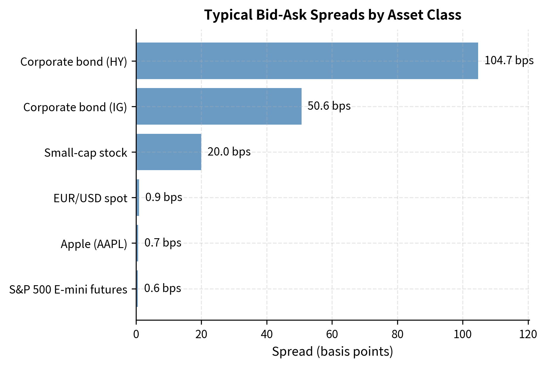
The variation across asset classes is substantial. Liquid large-cap equities and major FX pairs trade with spreads of 1-2 basis points, while corporate bonds can have spreads of 50-100+ basis points. This difference has major implications for strategy design: a high-turnover strategy might be profitable in SPY but disastrous in small-cap or corporate bond markets.
Slippage and Price Impact
Slippage refers to the difference between the expected execution price (such as the price at the time of order submission) and the actual execution price. This concept captures the reality that markets move between the moment you decide to trade and the moment your order is filled. Slippage arises from two sources:
-
Time-based slippage: Prices move between when you decide to trade and when your order is executed. This is particularly relevant for strategies with execution delays.
-
Market impact slippage: Your order itself moves the market price against you because you consume available liquidity at the best prices and must execute deeper into the order book.
For small orders that can be filled at the best bid or ask, slippage is minimal. But as order size increases relative to available liquidity, market impact becomes the dominant transaction cost component. Understanding this transition from "small order, minimal impact" to "large order, significant impact" is crucial for managing execution costs effectively.
This example illustrates how slippage grows nonlinearly with order size. A 100-share order executes at the best ask price with zero slippage, while a 10,000-share order must consume multiple price levels, resulting in significant slippage. This nonlinearity is a fundamental feature of market impact that we will model more rigorously in the next section.
Key Parameters
The key parameters for analyzing transaction costs are:
- Commission: Explicit fees paid to brokers for executing trades.
- Spread: The difference between the ask and bid prices (). Represents the cost of immediate execution.
- Slippage: The difference between the expected execution price and the actual execution price.
- VWAP: Volume-Weighted Average Price. The average price achieved when executing an order across multiple price levels.
Market Impact Modeling
Market impact is a critical and complex transaction cost component to model. When you trade, you are not simply paying a fixed cost; you are changing the market price itself. This effect is temporary (prices revert after your trading pressure subsides) and permanent (your trades may convey information that is incorporated into prices). The challenge in modeling market impact lies in its dual nature: part of the price change is a mechanical response to consuming liquidity, which fades as the market rebalances, while another part reflects genuine information transmission that permanently updates the market's view of fair value.
Temporary vs. Permanent Impact
Temporary impact is the transient price displacement caused by trading pressure that reverts after trading ceases. It reflects the liquidity premium demanded by counterparties for absorbing your order flow.
Permanent impact is the lasting price change that remains after temporary impact has decayed. It reflects the information content of your trades that becomes incorporated into the market price.
The distinction is critical for execution strategy. If impact were purely temporary, you could simply wait for prices to revert before trading again. But permanent impact means that your early trades adversely affect your later trades, as the price has permanently moved against you. Consider a fund liquidating a large position: temporary impact means they pay a premium for immediate execution, but this premium disappears once they stop trading. Permanent impact, however, means that each sale drives down the price level at which subsequent sales occur, creating a compounding cost that cannot be avoided by waiting.
Empirical research, starting with the seminal work of Kyle (1985) and later Almgren and Chriss (2001), has established several stylized facts about market impact:
- Impact is concave in trade size: doubling the trade size does not double the impact
- Impact depends on the participation rate (fraction of market volume)
- Temporary impact decays over time, typically within minutes to hours
- Permanent impact persists and is related to the information content of trades
These empirical regularities provide the foundation for the mathematical models we develop next. The concavity of impact in trade size is particularly important: it means that large trades are more efficient per share than small trades in terms of impact cost, but total impact still grows with order size. This creates interesting tradeoffs in execution strategy that we will explore.
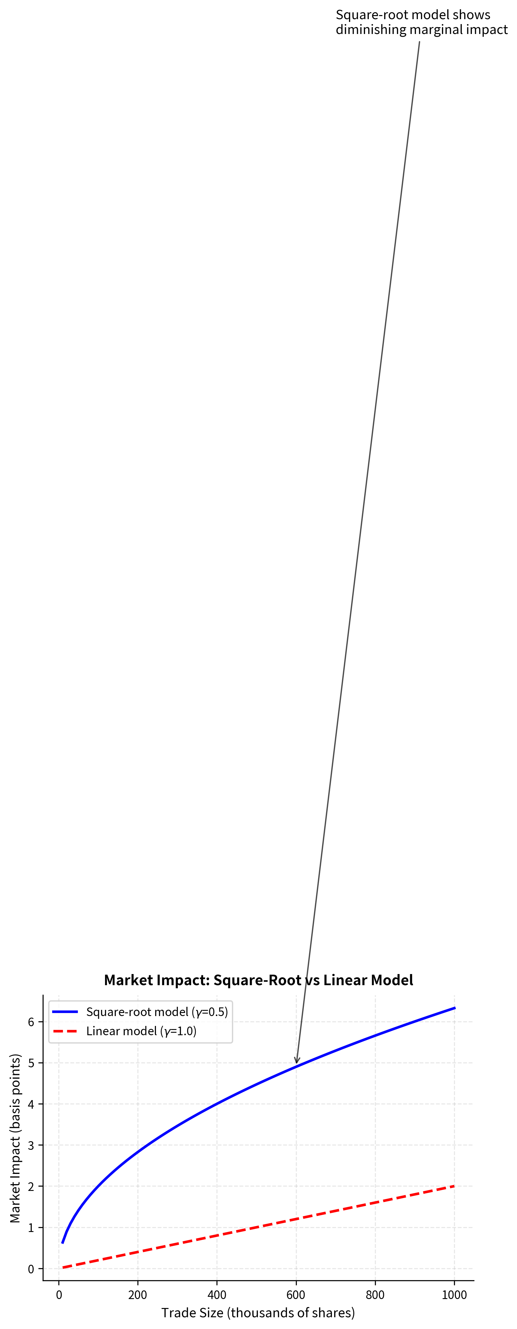
The Square-Root Model
The most widely used market impact model in practice is the square-root model. This model emerged from extensive empirical studies across equity, futures, and foreign exchange markets, and has proven remarkably robust across different asset classes and time periods. The model states that market impact scales with the square root of the trade size relative to market volume:
where:
- : market impact cost as a fraction of price
- : daily volatility of the asset
- : quantity traded (shares or dollars)
- : daily trading volume (in the same units as )
- : impact coefficient (market-dependent parameter)
- : impact exponent, empirically found to be approximately 0.5 (hence "square-root")
Let us examine each component of this formula to understand its economic intuition. The volatility term appears because impact is fundamentally about price uncertainty: in a more volatile market, liquidity providers demand greater compensation for taking the other side of your trade, since the risk of adverse price movement is higher. The participation rate captures how much of the market's trading activity your order represents; trading 10% of daily volume creates far more impact than trading 0.1%.
The impact coefficient is an empirical parameter that varies by market and must be estimated from data. Typical values range from 0.05 to 0.3 depending on the asset class and market conditions. Illiquid markets tend to have higher values, reflecting the greater difficulty of absorbing large orders without moving prices.
The square-root relationship, captured by the exponent , has been documented across many markets and time periods. It implies that trading 4% of daily volume incurs only about twice the impact of trading 1%, not four times. This sublinearity is crucial for understanding strategy capacity. Mathematically, if you trade four times the volume ( instead of ), your impact becomes , which is only twice the original impact despite quadrupling the trade size.
The square-root relationship has important practical implications. Consider a fund that has been trading 1% of daily volume with satisfactory performance. If they decide to double their capital, trading 2% of daily volume, their impact costs increase by a factor of , not 2. This is good news for scaling strategies, but the costs still grow faster than linearly would suggest in absolute dollar terms.
The Almgren-Chriss Framework
For optimal execution of large orders, we need a more sophisticated model that captures the tradeoff between market impact and timing risk. The Almgren-Chriss framework, introduced in their influential 2001 paper, provides exactly this. This framework transformed the field by formalizing the execution problem as a mathematical optimization: how should we balance the certainty of market impact costs against the uncertainty of price movements during execution?
Consider if you must liquidate X shares over a time horizon . The key insight is that you face a fundamental dilemma. Trading quickly minimizes your exposure to adverse price movements but concentrates all of the market impact into a short period. Trading slowly spreads out the impact but leaves you vulnerable to volatility risk as prices may move against you while you still hold a large position.
Let the trading trajectory be described by , the number of shares remaining to be sold at time , with and . The trading rate is . This notation captures the complete execution path: at any moment, we know both how many shares remain and how fast we are trading.
The framework models two sources of cost, corresponding to the temporary and permanent impact we discussed earlier:
Permanent impact: The price reflects the cumulative effect of past trading:
where:
- : asset price at time
- : initial asset price
- : permanent impact drift function
- : trading rate at time
- : current time
This equation captures how the market price drifts downward (for a sell program) as our trading activity reveals information. The function describes how the trading rate translates into price pressure. The integral accumulates all past trading pressure, reflecting that permanent impact is indeed permanent: the price remembers all our previous trades.
Temporary impact: Additionally, each trade temporarily depresses the price:
where:
- : effective execution price
- : fundamental asset price
- : temporary impact function
- : trading rate
While permanent impact accumulates over time, temporary impact depends only on our current trading rate. The function captures the instantaneous price concession we must offer to attract counterparties. The faster we trade, the larger this concession must be to induce sufficient liquidity providers to take the other side.
We can derive the expected execution cost by calculating the Implementation Shortfall which is the difference between the initial portfolio value and the total proceeds from liquidation. This measure, introduced by Perold in 1988, has become the industry standard for execution cost measurement because it captures the complete cost of implementing an investment decision.
The total proceeds correspond to the integral of the execution price multiplied by the trading rate (negative for sales):
The first term represents the proceeds if we could execute at the fundamental price , while the second term represents the additional cost from temporary impact. Note that the trading rate is negative for sales (shares remaining is decreasing), which is why we use the absolute value in the second integral to ensure temporary impact is always a cost.
Using integration by parts on the first term , we set and , which implies and . The integration yields:
The boundary conditions enforce that we start with shares and end with zero. The price dynamics equation tells us that the price falls by for each unit of trading rate.
Negating this result provides the first term of the proceeds equation:
Subtracting the proceeds from the initial value yields the total expected cost:
where:
- : expected total execution cost
- : liquidation time horizon
- : permanent impact component
- : temporary impact component
- : shares remaining at time
- : trading rate
The integral sums two distinct cost sources:
- : The cost from permanent price drift, which devalues the entire remaining position .
- : The cost from temporary impact, which acts as a direct toll on the specific shares traded at each moment.
This decomposition reveals a crucial asymmetry. Permanent impact costs are amplified by the remaining position: when you have many shares left to sell, each unit of permanent price decline costs you more because it affects more shares. Temporary impact, by contrast, is a local cost that affects only the shares currently being traded.
The variance of execution cost (timing risk) depends on the price volatility and the remaining position:
where:
- : variance of execution cost
- : price volatility parameter
- : shares remaining at time
- : total time horizon
This formula captures the intuition that timing risk is proportional to how much position you hold and for how long. The squared term reflects that larger positions create proportionally more variance. If you liquidate quickly (small x(t) for most of the period), you have low variance, while if you hold a large position until late in the trading period, you have high variance.
You face a tradeoff: trading quickly minimizes timing risk but maximizes market impact; trading slowly minimizes impact but exposes the position to price volatility.
To implement this model, we often assume linear forms for the impact functions, which leads to the closed-form solutions used in the following example:
where:
- : permanent impact coefficient (distinct from the exponent in the square-root model)
- : temporary impact coefficient
- : trading rate
The linear assumption is a simplification, but it yields closed-form optimal strategies. More realistic nonlinear impact functions require numerical optimization, but the qualitative insights from the linear case carry over.
Under these assumptions, the total permanent impact cost depends only on the total shares traded, making it path-independent. The optimization problem therefore simplifies to balancing temporary impact costs against volatility risk.
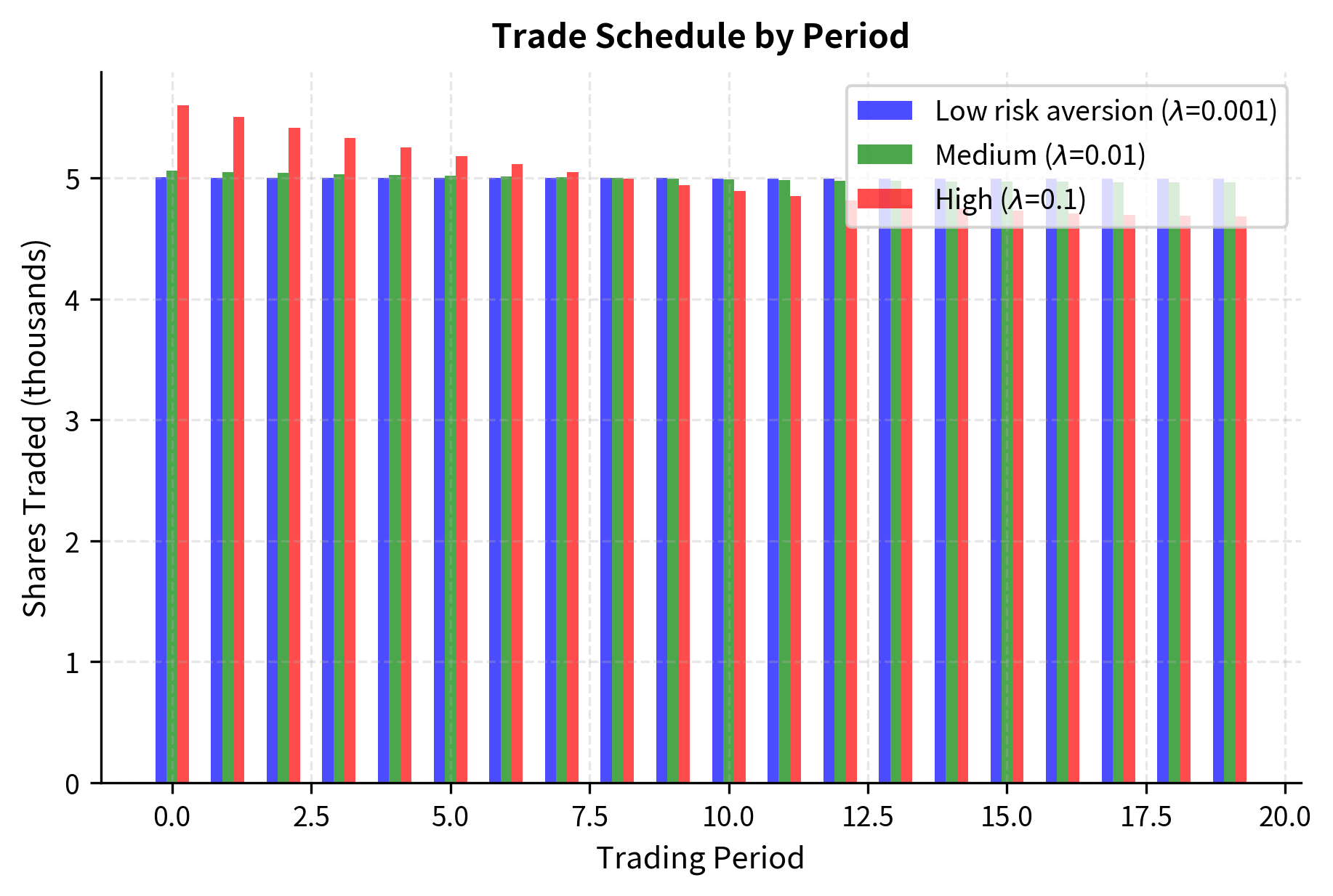
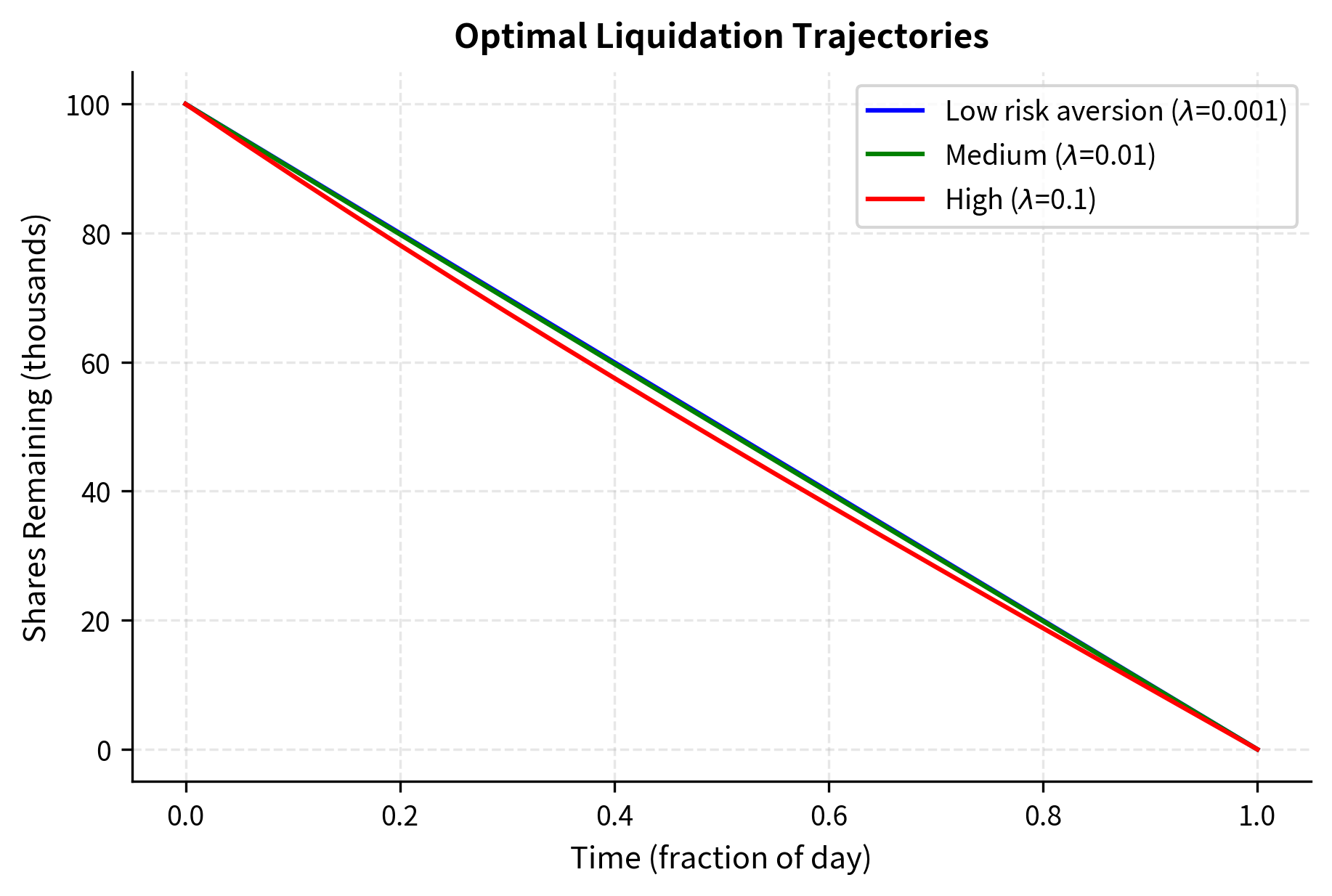
The key insight from the Almgren-Chriss model is that optimal execution depends critically on the tradeoff between market impact and timing risk. If you are risk-neutral, you would spread execution evenly over time (TWAP), while if you are risk-averse, you front-load execution to reduce exposure to volatility. We'll explore execution algorithms that implement these ideas in detail in the upcoming chapter on execution algorithms and optimal execution.
Key Parameters
The key parameters for market impact models are:
- ̒ (Sigma): Daily volatility of the asset. Higher volatility implies higher risk for liquidity providers, resulting in larger spreads and impact costs.
- (Volume): Average daily trading volume. This normalizes the trade size; the same dollar trade has less impact in a high-volume stock.
- ̑ (Eta): Impact coefficient. A market-specific parameter scaling the overall cost (typically 0.1 to 0.3).
- ̓ (Gamma): Impact exponent. In the square-root model, , indicating that impact costs increase with the square root of trade size.
- ̒ (Lambda): Risk aversion parameter (Almgren-Chriss). Determines the optimal trading speed by balancing impact cost (slow trading) against volatility risk (fast trading).
Estimating Transaction Cost Parameters
Modeling transaction costs requires estimating the relevant parameters from market data. These parameters vary across assets, time periods, and market conditions. Accurate estimation is essential for realistic backtesting and strategy evaluation. The challenge lies in the fact that we can only observe transaction costs for trades we actually execute, and these observations are inherently noisy due to the many factors influencing each individual trade. Nevertheless, systematic approaches to estimation can yield useful parameter values that significantly improve our cost models.
Spread Estimation
The bid-ask spread can be estimated directly from quote data or inferred from trade data when quotes are unavailable. The choice of method depends on the data available and the precision required.
From quote data: The quoted spread at time is simply:
where:
- : quoted spread at time
- : lowest sell price
- : highest buy price
This direct measurement is straightforward when high-frequency quote data is available. However, the quoted spread may overstate actual trading costs if orders execute at prices better than the posted quotes, a phenomenon called price improvement.
The effective spread, which accounts for orders that execute at prices better than the quoted spread, is calculated from trade data:
where:
- : effective spread
- : direction indicator (+1 for buys, -1 for sells)
- : trade price
- : quote midpoint at trade time
The factor of 2 appears because we measure the distance from the midpoint to the execution price, which represents half the round-trip cost. Multiplying by the direction indicator ensures that the spread is positive regardless of whether the trade was a buy or a sell. A buy trade should execute above the midpoint (positive deviation), while a sell trade should execute below (negative deviation), so the direction indicator aligns these cases.
Roll's spread estimator: When quote data is unavailable, Roll (1984) showed that the spread can be estimated from the autocovariance of price changes:
where:
- : estimated effective spread
- : covariance operator
- : price change ()
This estimator relies on the fact that bid-ask bounce creates negative serial correlation in observed price changes. If the true value is stable, a buy trade executed at the ask followed by a sell trade at the bid results in a negative price change, while a sell followed by a buy results in a positive change. This oscillation creates a negative covariance proportional to the square of the spread.
When prices bounce between bid and ask without any change in fundamental value, consecutive returns tend to have opposite signs: an uptick to the ask is often followed by a downtick to the bid, and vice versa. This bid-ask bounce creates a predictable negative correlation. Roll showed that under idealized conditions, the covariance equals , where is the spread, which leads directly to the estimator above.
The Roll estimator closely approximates the true spread using only close-to-close price data. This demonstrates how transaction costs can be inferred from price dynamics even when high-frequency quote data is unavailable, though the estimate becomes noisy in the absence of a strong bid-ask bounce signal.
Impact Parameter Estimation
Estimating market impact parameters requires data on trade sizes, volumes, and subsequent price movements. The typical approach is to regress observed price changes on participation rates. This regression framework allows us to estimate both the impact coefficient and the impact exponent simultaneously.
For the square-root model, taking logs transforms the relationship into a linear regression:
where:
- : market impact cost
- : asset volatility
- : impact coefficient
- : impact exponent
- : trade quantity
- : daily trading volume
This allows estimation of both and using standard regression techniques. The slope of the regression in log-log space directly estimates , while the intercept allows us to back out once we know the volatility. This linearization is powerful because it transforms a potentially complex nonlinear estimation problem into a simple ordinary least squares regression.
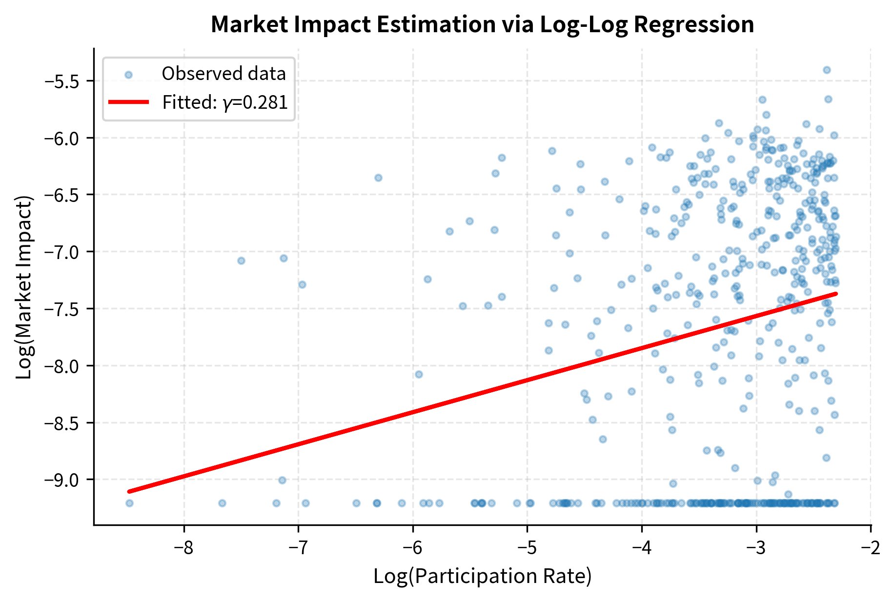
The regression successfully recovers the true parameters with high accuracy, validating the log-linear relationship between participation rate and market impact. The fitted line in the log-log plot confirms that the square-root law () holds for the simulated data.
In practice, impact parameter estimation is complicated by selection bias (you only observe impacts for trades you actually made), endogeneity (your trading strategy depends on expected costs), and non-stationarity (parameters vary over time). Sophisticated estimation methods address these issues, but even simple estimates provide valuable guidance for strategy development.
Key Parameters
The key parameters for transaction cost estimation are:
- : Effective spread. Captures the cost of immediate execution relative to the midpoint.
- Cov: Autocovariance of price changes. Used in Roll's estimator to infer spread from price dynamics.
- ̑: Impact coefficient estimated from regression.
- ̓: Impact exponent. The slope of the regression line in log-log space.
- : Participation rate. The independent variable in impact modeling.
Incorporating Costs in Strategy Design
With a framework for understanding and estimating transaction costs, we can now address the critical question: how should costs be incorporated into strategy development and backtesting? The answer determines which strategies are viable, how much capital they can manage, and what returns investors should expect.
The Turnover-Cost Relationship
Turnover measures how frequently a portfolio is traded, typically expressed as an annual percentage of portfolio value. A portfolio with 200% annual turnover means the entire portfolio is bought and sold twice during the year. This metric is crucial because it directly links strategy characteristics to transaction costs: a strategy's turnover, combined with its cost per trade, determines its total annual transaction cost burden.
Portfolio Turnover is calculated as the sum of all buys (or equivalently, all sells) during a period divided by the average portfolio value:
where:
- : annualized portfolio turnover ratio
- : sum of absolute values of all buy and sell trades
- : mean capital invested during the period The division by 2 accounts for the fact that each rebalancing trade involves both a buy and a sell.
The relationship between turnover and costs is straightforward but often underappreciated:
where:
- : total transaction costs per year as a percentage of portfolio value
- : annualized portfolio turnover ratio
- : average round-trip execution cost as a percentage of trade value
For a strategy with 200% annual turnover and 10 basis points round-trip cost per trade, annual transaction costs are 0.2% of portfolio value. This is a significant drag on performance. A strategy must generate more than 0.2% alpha just to break even. This formula establishes a direct link between trading frequency and cost.
This analysis shows that high-turnover strategies require either very large gross alpha or very low transaction costs to be viable. The statistical arbitrage strategy with 5000% turnover consumes roughly 17% of its alpha in transaction costs, while the high-frequency strategy must achieve 50% gross alpha just to net 40% after costs on 100,000% turnover.
Breakeven Analysis
A valuable exercise in strategy development is calculating the breakeven cost level, which is the transaction cost at which your strategy's net alpha equals zero. This calculation provides a critical threshold: if your estimated transaction costs exceed this level, the strategy cannot be profitable regardless of how compelling its theoretical foundation.
where:
- : transaction cost level where net alpha is zero
- : expected strategy return before costs
- : annualized portfolio turnover
If the estimated transaction cost exceeds this breakeven level, the strategy is not viable. This formula filters strategy ideas. Before investing development time, compare the breakeven cost to realistic cost estimates.
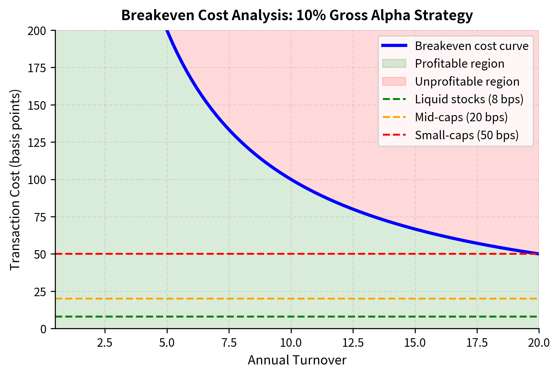
The chart illustrates strategy viability across different market conditions. With 10% gross alpha, a strategy can afford 125 basis points of cost at 8x turnover, but only 50 basis points at 20x turnover. The horizontal lines show that this strategy would be profitable in liquid stocks at most turnover levels, but becomes unprofitable in small-caps at turnover above about 20x.
Cost-Aware Backtesting
As discussed in the previous chapter on backtesting, incorporating realistic transaction costs is essential for reliable strategy evaluation. Here we provide a practical implementation for cost-aware backtesting
The results demonstrate how transaction costs transform strategy performance. A strategy showing a 30% gross return and Sharpe ratio above 1.5 can be reduced to single-digit returns and sub-1 Sharpe when realistic costs are applied. This is precisely why cost modeling is non-negotiable in serious strategy development.
Cost-Aware Portfolio Optimization
Building on the portfolio optimization techniques from Part IV, we can incorporate transaction costs directly into the optimization objective. The traditional mean-variance optimization minimizes:
where:
- : optimal weight vector
- : portfolio weight vector
- : covariance matrix of asset returns
- : risk aversion parameter
- : vector of expected returns
This classical formulation treats portfolio construction as a static problem: given expected returns and covariances, find the best weights. But in practice, we start from an existing portfolio, and reaching the theoretically optimal weights requires trading. If transaction costs are significant, the cost of getting to the optimal portfolio may outweigh the benefit of being there.
With transaction costs, we add a penalty for trading:
where:
- : optimal weight vector
- : portfolio weight vector
- : covariance matrix of asset returns
- : risk aversion parameter
- : vector of expected returns
- : transaction cost parameter
- : L1 norm representing total traded weight (sum of absolute changes)
- : vector of current portfolio weights
The L1 norm sums the absolute values of all weight changes, which directly represents the total trading volume needed to move from the current portfolio to the new weights. The parameter scales how much we penalize this trading.
This modification creates a "no-trade region" around the current portfolio: small changes in expected returns or covariances will not trigger rebalancing if the improvement is insufficient to cover transaction costs. The optimizer essentially asks: is the benefit of moving to a slightly better portfolio worth the cost of getting there? When is large, the answer is often no, and the optimizer makes smaller adjustments.
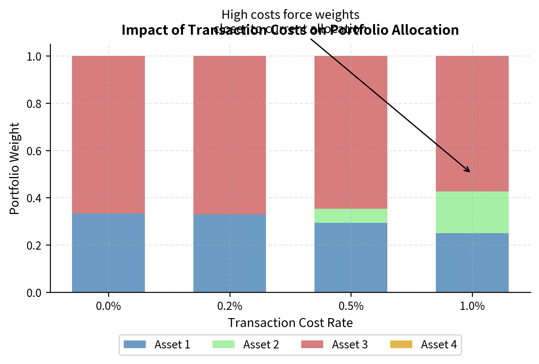
As transaction costs increase, the optimizer becomes more reluctant to deviate from the current portfolio. At 0% cost, it rebalances significantly toward the high-return Asset 3. At 1% cost, the optimizer barely moves from equal weights because the cost of rebalancing outweighs the expected benefit.
Key Parameters
The key parameters for cost-aware strategy design are:
- Turnover: Annual trading volume as a percentage of portfolio value. The primary driver of total transaction costs.
- Cost per Trade: The average cost (explicit + implicit) incurred for each trade.
- Breakeven Cost: The transaction cost level at which a strategy's net alpha becomes zero.
- c: Transaction cost parameter in portfolio optimization. Acts as a penalty on rebalancing volume.
- ̒: Risk aversion parameter. Balances the trade-off between expected return and portfolio variance.
Practical Implementation: Complete Cost Model
Let's now build a comprehensive transaction cost model that combines all the elements we've discussed: explicit costs, spread costs, and market impact.
The analysis reveals the dramatic differences in trading costs across market segments. For a 100,000-share trade, large-cap stocks incur about 6 basis points total cost, while small-caps cost over 100 basis points, a seventeen-fold difference. Market impact dominates the cost structure for larger trades in less liquid markets.
Key Parameters
The key parameters for the Transaction Cost Model are:
- Commission: Explicit fee per share or per trade.
- Spread: Bid-ask spread in basis points. This captures the cost of crossing the spread for immediate execution.
- ̑: Market impact coefficient. Scales the impact relative to volatility and participation rate.
- ̓: Market impact exponent. Determines the curvature of the price impact function.
- Participation Rate: Ratio of trade size to daily volume (). A primary driver of market impact costs.
Strategy Capacity and Scalability
Understanding transaction costs leads naturally to questions about strategy capacity: how much capital can a strategy manage before costs erode its edge? This question is central to both strategy development and fund management. A strategy that generates attractive returns at small scale may become mediocre or even unprofitable at larger scale due to the nonlinear relationship between trade size and impact costs.
Strategy Capacity is the maximum capital a strategy can manage while maintaining acceptable risk-adjusted returns. Beyond this capacity, market impact costs grow faster than the alpha generated, causing net performance to deteriorate.
The square-root impact model implies that market impact grows with the square root of trade size, but total impact (in dollars) grows with size raised to the power , typically around . This means doubling your capital roughly triples your impact costs, creating a natural ceiling on strategy size. To understand this relationship mathematically, consider that impact per dollar traded scales as where . When you double your capital, you double , so impact per dollar becomes times larger. But you're also trading twice as many dollars, so total impact costs become times larger, which is roughly tripling.
The low-turnover value strategy has essentially unlimited capacity because its trading costs are minimal. In contrast, the high-turnover intraday momentum strategy can only manage several million before impact costs erode its edge. This explains why some of the most successful strategies remain small and capacity-constrained.
Key Parameters
The key parameters for strategy capacity estimation are:
- Gross Alpha: Expected strategy return before costs. Higher alpha supports higher capacity.
- Turnover: Annual portfolio turnover. High turnover rapidly consumes alpha through transaction costs.
- (Volume): Daily trading volume. Strategies are constrained by the available liquidity in their target assets.
- ̒: Asset volatility. Higher volatility implies higher market impact costs.
- Minimum Net Alpha: The performance floor required for the strategy to be considered viable.
Limitations and Practical Considerations
While the models presented in this chapter provide valuable frameworks for understanding and estimating transaction costs, several important limitations deserve attention.
Model Uncertainty and Parameter Stability
Transaction cost parameters are not constants; they vary with market conditions, time of day, and broader volatility regimes. The square-root exponent is an empirical average that can range from 0.3 to 0.7 depending on the market and time period. Impact coefficients vary even more widely. A model calibrated during normal market conditions may dramatically underestimate costs during periods of stress or low liquidity.
This parameter uncertainty compounds with the inherent noisiness of cost measurement. Individual trades have highly variable execution quality due to randomness in order flow, market maker inventory, and timing. Reliable estimates require large samples, but by the time you have enough data, the market may have changed.
Execution Quality Beyond the Model
The models presented assume a passive approach where you accept market prices. In practice, execution algorithms can significantly reduce costs through techniques like:
- Splitting orders to reduce instantaneous impact
- Using limit orders to capture spread instead of paying it
- Timing execution to coincide with periods of high liquidity
- Exploiting dark pools and alternative venues
These techniques, covered in the upcoming chapter on execution algorithms, can reduce realized costs below what simple models predict, but they also introduce new complexities and potential failure modes.
Strategic Interaction and Information Leakage
The market impact models presented treat impact as a function of trade size alone, ignoring the strategic environment. In reality, other market participants observe and react to your trading. Predictable execution patterns can be exploited by high-frequency traders; information about your intentions can leak through broker channels or observable patterns.
For large institutional traders, information leakage can be a cost equal to or greater than direct market impact. This is another reason why actual trading costs often exceed model predictions, particularly for traders with significant market presence.
Cost-Alpha Interaction
A subtle but important issue is that transaction costs and alpha are not independent. High-alpha opportunities often arise precisely in situations where costs are also high: illiquid markets, stressed conditions, or concentrated positions. A strategy that only generates alpha when you need to trade large size in illiquid conditions may have much lower capacity than a naive cost model suggests.
Conversely, the act of trading on alpha erodes that alpha through information revelation. If your signal is truly informative, your trades will permanently move prices; the permanent impact component represents the market learning from your trading. This creates a fundamental tension between exploiting alpha quickly (before others discover it) and trading slowly (to minimize impact).
Summary
Transaction costs represent the gap between theoretical strategy returns and realized performance. This chapter has developed a comprehensive framework for understanding, measuring, and incorporating these costs into quantitative trading systems.
Key concepts covered include:
-
Types of transaction costs: Explicit costs (commissions, fees, taxes), bid-ask spreads, and market impact all contribute to the total cost of trading. For institutional-size trades, market impact typically dominates.
-
Market impact modeling: The square-root model captures the empirically observed relationship between trade size and price impact. The Almgren-Chriss framework extends this to optimal execution problems, balancing impact against timing risk.
-
Cost estimation: Spread can be estimated from quote data or inferred using Roll's estimator. Impact parameters are estimated via regression of observed costs on trade size and market conditions.
-
Strategy design implications: Transaction costs must be incorporated into backtesting for realistic performance estimates. Turnover analysis and breakeven calculations reveal whether a strategy's edge is sufficient to overcome its trading costs.
-
Capacity constraints: The nonlinear relationship between trade size and impact creates natural limits on strategy scale. High-turnover strategies typically have much lower capacity than low-turnover approaches.
Realistic cost modeling is essential for avoiding strategies that work in simulation but fail in production. The difference between gross and net performance often determines whether a strategy is profitable or not.
The next chapter explores market microstructure and order types, providing the foundation for understanding how orders interact with markets. This knowledge is essential for implementing the execution algorithms discussed later in Part VII.
Quiz
Ready to test your understanding? Take this quick quiz to reinforce what you've learned about transaction costs and market impact.

Comments