Backtesting & Simulation: Frameworks for Strategy Validation

Michael Brenndoerfer

Quantitative Finance Data, Analytics & AI Software Engineering

Master backtesting frameworks to validate trading strategies. Avoid look-ahead bias, measure risk-adjusted returns, and use walk-forward analysis for reliability.

Reading Level

Choose your expertise level to adjust how many terms are explained. Beginners see more tooltips, experts see fewer to maintain reading flow. Hover over underlined terms for instant definitions.

Backtesting and Simulation of Trading StrategiesLink Copied

Throughout Part VI, we developed a rich toolkit of quantitative trading strategies, from mean reversion and momentum to machine learning-based approaches. Two questions arise: would these strategies have been profitable historically, and will that performance translate to the future?

Backtesting evaluates a trading strategy by simulating its performance on historical data. It acts as a simulation tool to test ideas against past market conditions. A well-designed backtest reveals profitability, behavior during market stress, capital requirements, and the source of returns.

However, backtesting presents significant risks. The flexibility to test many ideas can lead to strategies that appear robust in hindsight but fail in live trading. Biases, data errors, and methodological flaws often create a discrepancy between simulated results and real-world profitability.

This chapter covers the complete backtesting workflow: building a simulation framework, avoiding common pitfalls, measuring performance rigorously, and testing whether your results generalize beyond the data you used to develop them. By the end, you'll understand not just how to run a backtest, but how to interpret one critically, a skill that separates you from those who fool themselves with beautiful but meaningless equity curves.

The Backtesting FrameworkLink Copied

A backtesting framework simulates the operation of a trading strategy through historical time. At each point in the past, the system must answer a fundamental question: what trades would the strategy have made given only the information available at that moment? This simple requirement, respecting the flow of time, is the foundation of all valid backtesting. The framework must faithfully reconstruct the decision-making environment that would have existed at each historical moment, using only the data that would have been observable then and applying the same rules consistently throughout the simulation period.

Core ComponentsLink Copied

Every backtesting system consists of five essential components that work together to produce simulated results. Understanding how these components interact is crucial for building reliable simulations and diagnosing problems when results seem too good to be true.

The core components are:

Historical Data: This includes price series, fundamental data, or alternative data. Data quality directly determines validity, as errors propagate through subsequent calculations. Clean, accurate, and properly aligned data forms the foundation of analysis.
Signal Generation: This logic transforms available information into trading decisions (buy, sell, or hold). This module encodes the strategy rules and must rely solely on information available at each specific time step.
Position Management: This layer converts signals into portfolio allocations, handling position sizing, rebalancing, and constraints. It translates abstract signals into concrete capital deployment.
Execution Simulation: This component models order fills, transaction costs, slippage, and market impact, bridging the gap between theoretical positions and realistic outcomes.
Performance Tracking: This records portfolio values and returns, maintaining the historical record required for statistical analysis and visualization.

The interaction between these components creates a simulation loop that processes one time step at a time. At each step, the system receives new market data, generates signals based on available information, converts those signals into target positions, simulates the execution of any required trades, and records the resulting portfolio state. This sequential processing mirrors how a real trading system operates, making it easier to ensure temporal consistency.

In[2]:

Code

import numpy as np


# Conceptual backtesting loop structure
def backtest_skeleton(prices, signal_function, initial_capital=100000):
    """
    Basic backtesting loop structure demonstrating the time-sequential process.

    At each time step, we:
    1. Generate signals from available data
    2. Convert signals to target positions
    3. Execute trades (simulate fills)
    4. Update portfolio state
    5. Record performance
    """
    n_periods = len(prices)

    # Initialize tracking arrays
    positions = np.zeros(n_periods)
    portfolio_value = np.zeros(n_periods)
    cash = initial_capital
    shares = 0

    for t in range(1, n_periods):
        # Only use data available up to time t-1 for decisions
        available_data = prices[:t]

        # Generate signal from available information only
        signal = signal_function(available_data)

        # Convert signal to target position (simplified)
        if signal > 0 and shares == 0:
            # Buy signal: invest all cash
            shares = cash / prices[t]
            cash = 0
        elif signal < 0 and shares > 0:
            # Sell signal: liquidate position
            cash = shares * prices[t]
            shares = 0

        # Record state
        positions[t] = shares
        portfolio_value[t] = cash + shares * prices[t]

    # Handle initial value
    portfolio_value[0] = initial_capital

    return portfolio_value, positions

import numpy as np


# Conceptual backtesting loop structure
def backtest_skeleton(prices, signal_function, initial_capital=100000):
    """
    Basic backtesting loop structure demonstrating the time-sequential process.

    At each time step, we:
    1. Generate signals from available data
    2. Convert signals to target positions
    3. Execute trades (simulate fills)
    4. Update portfolio state
    5. Record performance
    """
    n_periods = len(prices)

    # Initialize tracking arrays
    positions = np.zeros(n_periods)
    portfolio_value = np.zeros(n_periods)
    cash = initial_capital
    shares = 0

    for t in range(1, n_periods):
        # Only use data available up to time t-1 for decisions
        available_data = prices[:t]

        # Generate signal from available information only
        signal = signal_function(available_data)

        # Convert signal to target position (simplified)
        if signal > 0 and shares == 0:
            # Buy signal: invest all cash
            shares = cash / prices[t]
            cash = 0
        elif signal < 0 and shares > 0:
            # Sell signal: liquidate position
            cash = shares * prices[t]
            shares = 0

        # Record state
        positions[t] = shares
        portfolio_value[t] = cash + shares * prices[t]

    # Handle initial value
    portfolio_value[0] = initial_capital

    return portfolio_value, positions

Event-Driven vs Vectorized BacktestingLink Copied

Two architectural approaches dominate backtesting implementations, each with distinct advantages and trade-offs that make them suitable for different situations.

Event-driven backtesting processes data one event at a time, maintaining explicit state throughout the simulation. This approach mimics how a live trading system operates and naturally prevents look-ahead bias because each decision is made in isolation, using only information available at that moment. The explicit state management makes it straightforward to model complex portfolio dynamics, such as margin requirements, position limits, and multi-asset interactions. However, the sequential nature of event-driven processing makes it computationally slower than alternatives, and the additional complexity can introduce implementation bugs if not carefully managed.

Vectorized backtesting uses array operations to compute signals and positions across the entire dataset simultaneously. This approach leverages the highly optimized linear algebra libraries underlying NumPy and pandas to achieve dramatic speed improvements, often running hundreds of times faster than equivalent event-driven code. The concise syntax also makes strategies easier to read and verify. However, vectorized backtesting requires careful attention to prevent future information from leaking into past calculations. Time-alignment of arrays becomes critical, and a single misplaced index can introduce look-ahead bias that makes results meaningless.

In[3]:

Code

def vectorized_momentum_backtest(prices, lookback=20):
    """
    Vectorized backtest of a simple momentum strategy.

    Key: Use .shift() to ensure signals are based only on past data.
    The signal at time t uses returns from t-lookback to t-1.
    """
    returns = prices.pct_change()

    # Momentum signal: positive if past returns were positive
    # .shift(1) ensures we don't use today's return in today's signal
    momentum = returns.rolling(window=lookback).mean().shift(1)

    # Position: +1 when momentum positive, -1 when negative
    position = np.sign(momentum)

    # Strategy returns: position held * return realized
    # Since position is based on shifted momentum (t-1), it aligns with returns (t)
    strategy_returns = position * returns

    return strategy_returns.dropna()

def vectorized_momentum_backtest(prices, lookback=20):
    """
    Vectorized backtest of a simple momentum strategy.

    Key: Use .shift() to ensure signals are based only on past data.
    The signal at time t uses returns from t-lookback to t-1.
    """
    returns = prices.pct_change()

    # Momentum signal: positive if past returns were positive
    # .shift(1) ensures we don't use today's return in today's signal
    momentum = returns.rolling(window=lookback).mean().shift(1)

    # Position: +1 when momentum positive, -1 when negative
    position = np.sign(momentum)

    # Strategy returns: position held * return realized
    # Since position is based on shifted momentum (t-1), it aligns with returns (t)
    strategy_returns = position * returns

    return strategy_returns.dropna()

The shift(1) operations in the code above are essential for maintaining temporal integrity. They ensure that the position we hold today was determined by yesterday's signal, which in turn was computed from data available before yesterday's close. The first shift ensures the momentum calculation doesn't include today's return, while the second shift ensures we're measuring the return earned on a position that was already established. Any misalignment here introduces look-ahead bias, which would make the backtest results invalid and potentially misleading.

Data Requirements and AlignmentLink Copied

Proper data handling requires attention to several timing issues that can subtly corrupt backtest results if not addressed correctly. These issues arise because the data we observe today often differs from what was available in the past, and because different data sources may use different conventions for timestamps and adjustments.

The first concern is point-in-time accuracy. Financial databases often update historical records as new information becomes available, meaning the data you see today may differ significantly from what was available in the past. For example, earnings figures are frequently restated, economic indicators are revised, and index compositions change over time. If your backtest uses today's version of historical data, you may be implicitly assuming knowledge that wasn't available when the trading decisions would have been made. When available, use point-in-time databases that preserve the data exactly as it appeared on each historical date.

The second concern involves timestamp conventions. You must know whether your prices represent open, close, or some other time within the trading day. A strategy that trades on the close needs close prices, and using daily high prices would overstate returns by assuming you could consistently buy at the low and sell at the high. Similarly, be careful with time zones: a strategy trading US equities based on European market signals must account for the hours of overlap and delay between markets.

The third concern relates to corporate actions. Stock splits, dividends, and mergers change price series in ways that can distort return calculations if not handled properly. Use adjusted prices for return calculations to ensure that a 2-for-1 stock split doesn't appear as a 50% price drop. However, if your position sizing depends on share counts rather than dollar amounts, you may need raw prices to determine how many shares to trade.

In[4]:

Code

import numpy as np
import pandas as pd

# Generate sample price data for examples
np.random.seed(42)
n_days = 500

# Simulate two stocks with different characteristics
dates = pd.date_range(start="2020-01-01", periods=n_days, freq="B")
returns_1 = np.random.normal(0.0005, 0.02, n_days)  # Slight upward drift
returns_2 = np.random.normal(0.0003, 0.025, n_days)  # More volatile

# Create price series from returns
price_1 = 100 * np.cumprod(1 + returns_1)
price_2 = 100 * np.cumprod(1 + returns_2)

prices_df = pd.DataFrame({"Stock_A": price_1, "Stock_B": price_2}, index=dates)

import numpy as np
import pandas as pd

# Generate sample price data for examples
np.random.seed(42)
n_days = 500

# Simulate two stocks with different characteristics
dates = pd.date_range(start="2020-01-01", periods=n_days, freq="B")
returns_1 = np.random.normal(0.0005, 0.02, n_days)  # Slight upward drift
returns_2 = np.random.normal(0.0003, 0.025, n_days)  # More volatile

# Create price series from returns
price_1 = 100 * np.cumprod(1 + returns_1)
price_2 = 100 * np.cumprod(1 + returns_2)

prices_df = pd.DataFrame({"Stock_A": price_1, "Stock_B": price_2}, index=dates)

Out[5]:

Console

Sample price data (first 5 days):
               Stock_A     Stock_B
2020-01-01  101.043428  102.345444
2020-01-02  100.814536  107.261650
2020-01-03  102.170872  103.543512
2020-01-06  105.334143  105.031870
2020-01-07  104.893523  103.354924

Data spans 500 trading days from 2020-01-01 to 2021-11-30

The sample data confirms we have two aligned price series over 500 trading days. Ensuring correct timestamp alignment and data completeness is a prerequisite for any valid backtest. Before proceeding with strategy development, you should always verify that your data has no gaps, that prices are properly adjusted for corporate actions, and that the timestamps correspond to the market events your strategy depends on.

Biases in BacktestingLink Copied

The greatest danger in backtesting is self-deception. Historical data is finite, and with enough searching, you can find patterns that look profitable but arise purely from chance. These patterns reflect the random quirks of a particular dataset rather than any genuine market inefficiency that will persist into the future. Understanding the biases that afflict backtests is essential for producing results you can trust and for avoiding the costly mistake of deploying strategies that looked great in simulation but fail in live trading.

Look-Ahead BiasLink Copied

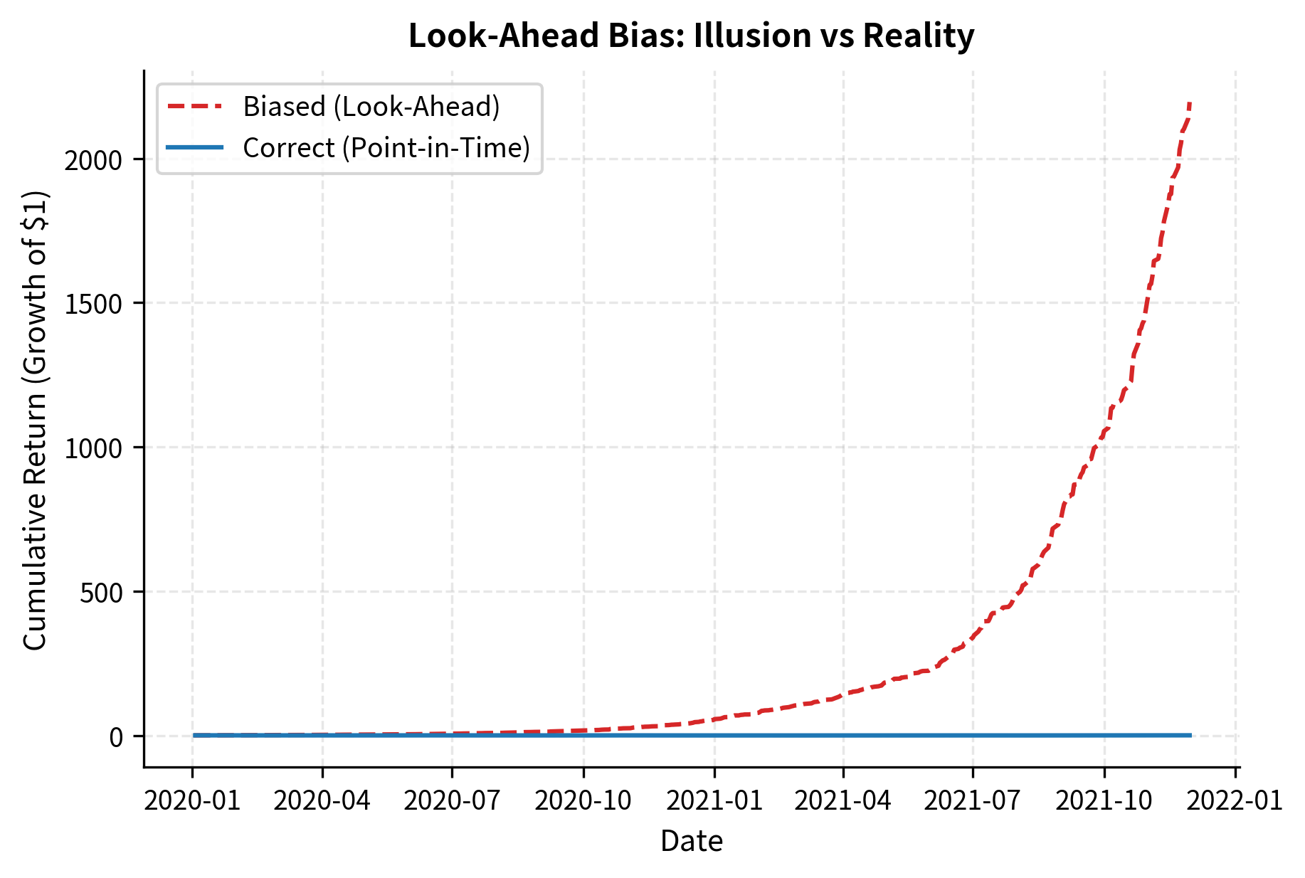
Look-ahead bias occurs when a backtest uses information that would not have been available at the time a trading decision was made. This is the most fundamental error in backtesting because it violates the causal structure of time. In the real world, you cannot use tomorrow's news to make today's trading decisions. But in a backtest, where all historical data sits in memory simultaneously, it's disturbingly easy to accidentally let future information leak into past calculations.

Common sources of look-ahead bias include several categories of errors that can creep into even carefully designed backtests.

Using future data in calculations: Computing a signal using today's price when it should be based on yesterday's close. This often results from off-by-one indexing errors or rolling calculations that include the current observation.
End-of-period knowledge: Using full-year earnings data at the start of the year when reports are released later. This assumes knowledge of figures before they are publicly available.
Restatements and revisions: Using revised economic or fundamental data (e.g., GDP, earnings) that was corrected months after the initial release, rather than the data actually available at the time.
Survivorship in filtering: Selecting a universe based on current criteria (e.g., "current top 100 stocks") rather than historical criteria, effectively filtering for companies that were successful enough to survive and grow.

In[6]:

Code

def demonstrate_look_ahead_bias(prices):
    """
    Demonstrate the difference between correct and biased signal generation.
    """
    returns = prices.pct_change()

    # WRONG: Using today's return to make today's decision
    # This is look-ahead bias - we're using future information
    biased_signal = np.sign(returns)  # Knows return before it happens
    biased_returns = biased_signal * returns  # Always profitable!

    # CORRECT: Using yesterday's return to make today's decision
    correct_signal = np.sign(returns.shift(1))  # Only past information
    correct_returns = correct_signal * returns  # Realistic performance

    return biased_returns, correct_returns


biased, correct = demonstrate_look_ahead_bias(prices_df["Stock_A"])

def demonstrate_look_ahead_bias(prices):
    """
    Demonstrate the difference between correct and biased signal generation.
    """
    returns = prices.pct_change()

    # WRONG: Using today's return to make today's decision
    # This is look-ahead bias - we're using future information
    biased_signal = np.sign(returns)  # Knows return before it happens
    biased_returns = biased_signal * returns  # Always profitable!

    # CORRECT: Using yesterday's return to make today's decision
    correct_signal = np.sign(returns.shift(1))  # Only past information
    correct_returns = correct_signal * returns  # Realistic performance

    return biased_returns, correct_returns


biased, correct = demonstrate_look_ahead_bias(prices_df["Stock_A"])

Out[7]:

Console

Impact of Look-Ahead Bias:
  Biased backtest (using future info):   Mean daily return = 1.5608%
  Correct backtest (using past only):    Mean daily return = 0.0373%

The biased version looks incredible but is physically impossible!

The biased version achieves high returns because it uses future information to determine trade direction. No real strategy can achieve this level of performance, yet subtle forms of look-ahead bias appear in many backtests. The biased strategy relies on foresight, making it profitable in simulation but unreplicable in practice. When you see backtest results that seem too good to be true, look-ahead bias should be your first suspicion.

Out[8]:

Visualization

Equity curves comparing a biased backtest (red) using future information against a correct point-in-time backtest (blue). The biased strategy shows impossible, smooth growth, illustrating how look-ahead bias creates an illusion of risk-free profitability.

Survivorship BiasLink Copied

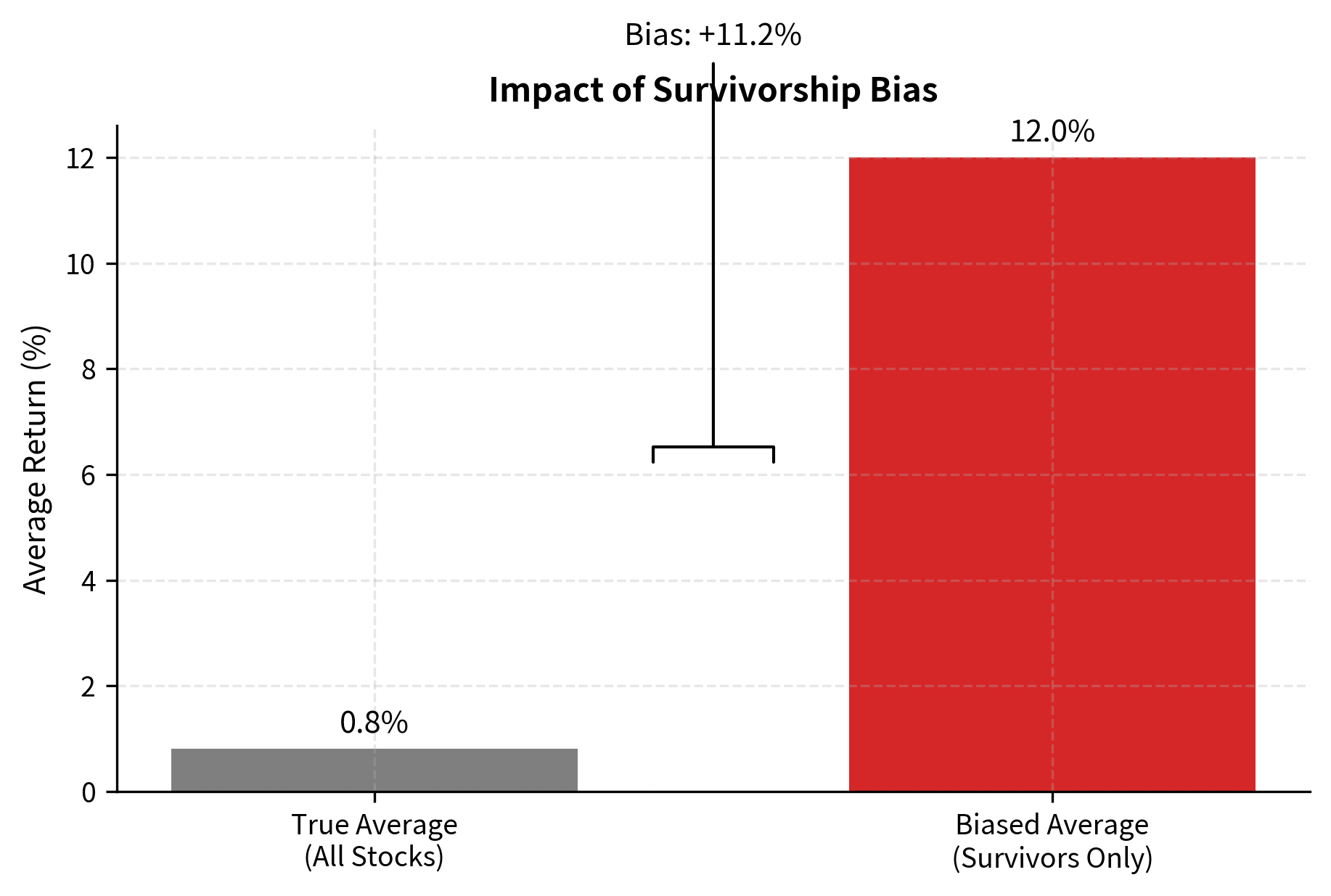
Survivorship bias occurs when your backtest only includes assets that survived to the present day, excluding those that were delisted, went bankrupt, or were acquired. This systematically overstates returns because failed investments become invisible in the historical record. You only see the winners, which makes the average past performance look better than it actually was.

Consider testing a strategy on "S&P 500 stocks" using today's index constituents. Companies currently in the index are, by definition, successful: they've grown large enough to be included and have avoided the failures that would have caused delisting. But a strategy trading in 2010 would have held different companies, including some that subsequently went bankrupt, were acquired at distressed prices, or shrank enough to be removed from the index. By testing only on survivors, you implicitly give your strategy perfect foresight about which companies to avoid, making your backtested returns look better than you could have achieved.

The magnitude of survivorship bias can be substantial. Academic research has shown that survivorship bias can add several percentage points per year to apparent returns in equity backtests. The effect is particularly pronounced for strategies that involve small-cap stocks, distressed securities, or other areas where failure rates are high.

In[9]:

Code

def simulate_survivorship_bias(n_stocks=100, n_periods=252, failure_rate=0.10):
    """
    Simulate the impact of survivorship bias on backtested returns.

    A fraction of stocks will "fail" (go to zero) during the simulation.
    We compare average returns including vs excluding failed stocks.
    """
    np.random.seed(123)

    # Generate returns for all stocks
    all_returns = np.random.normal(0.0003, 0.02, (n_stocks, n_periods))

    # Randomly select stocks that will fail
    n_failures = int(n_stocks * failure_rate)
    failed_stocks = np.random.choice(n_stocks, n_failures, replace=False)

    # Failed stocks have a large negative return at a random point
    for stock in failed_stocks:
        failure_day = np.random.randint(50, n_periods - 1)
        all_returns[stock, failure_day] = -1.0  # Complete loss
        all_returns[stock, failure_day + 1 :] = (
            0  # No more returns after failure
        )

    # Calculate cumulative returns
    cumulative = np.cumprod(1 + all_returns, axis=1)
    final_values = cumulative[:, -1]

    # Survivors are stocks with positive final value
    survivors = final_values > 0.01

    # Average return calculation
    all_stock_return = (final_values.mean() - 1) * 100
    survivor_return = (final_values[survivors].mean() - 1) * 100

    return all_stock_return, survivor_return, survivors.sum()


all_return, survivor_return, n_survivors = simulate_survivorship_bias()

def simulate_survivorship_bias(n_stocks=100, n_periods=252, failure_rate=0.10):
    """
    Simulate the impact of survivorship bias on backtested returns.

    A fraction of stocks will "fail" (go to zero) during the simulation.
    We compare average returns including vs excluding failed stocks.
    """
    np.random.seed(123)

    # Generate returns for all stocks
    all_returns = np.random.normal(0.0003, 0.02, (n_stocks, n_periods))

    # Randomly select stocks that will fail
    n_failures = int(n_stocks * failure_rate)
    failed_stocks = np.random.choice(n_stocks, n_failures, replace=False)

    # Failed stocks have a large negative return at a random point
    for stock in failed_stocks:
        failure_day = np.random.randint(50, n_periods - 1)
        all_returns[stock, failure_day] = -1.0  # Complete loss
        all_returns[stock, failure_day + 1 :] = (
            0  # No more returns after failure
        )

    # Calculate cumulative returns
    cumulative = np.cumprod(1 + all_returns, axis=1)
    final_values = cumulative[:, -1]

    # Survivors are stocks with positive final value
    survivors = final_values > 0.01

    # Average return calculation
    all_stock_return = (final_values.mean() - 1) * 100
    survivor_return = (final_values[survivors].mean() - 1) * 100

    return all_stock_return, survivor_return, survivors.sum()


all_return, survivor_return, n_survivors = simulate_survivorship_bias()

Out[10]:

Console

Survivorship Bias Demonstration:
  Number of stocks that survived: 90 out of 100
  Average return including all stocks: 0.8%
  Average return using survivors only: 12.0%

The survivor-only backtest overstates returns by 11.2 percentage points!

Out[11]:

Visualization

Comparison of average returns between the full investment universe and a survivor-only subset. The survivor-biased metric significantly overstates performance by excluding failed assets, demonstrating the importance of using point-in-time data.

To avoid survivorship bias, use point-in-time databases that include delisted securities, such as CRSP or similar academic databases that preserve the complete historical record. When such databases aren't available, explicitly track when securities exit your investment universe and include their terminal returns in your calculations. This means recording the final price at which a delisted stock traded, or the acquisition price in a merger, rather than simply dropping the security from your dataset.

Overfitting and Data SnoopingLink Copied

Overfitting occurs when a strategy's parameters are tuned too precisely to historical data, capturing noise rather than genuine patterns. A strategy with many adjustable parameters can always be made to fit past data perfectly, because with enough flexibility, you can find a configuration that would have profited from the specific sequence of price movements that happened to occur. However, such over-optimized strategies typically fail in live trading because the idiosyncratic patterns they exploit are random coincidences that won't repeat.

Overfitting

Overfitting is the tendency of a model with too many degrees of freedom to fit the idiosyncratic features of a particular dataset rather than the underlying signal. In backtesting, an overfit strategy exploits historical coincidences that won't repeat. The strategy has learned the noise in the training data rather than the signal, and this noise-fitting provides no predictive power for future market behavior.

The problem intensifies through data snooping, which occurs when you test many strategies on the same dataset and select the best performer. Even if each individual strategy is reasonable and based on sound economic intuition, selecting the winner from a large pool of candidates introduces statistical bias. You're effectively optimizing across all strategies simultaneously, and the "best" strategy may simply be the one that happened to fit the random patterns in your particular dataset most closely.

To understand why this happens, consider that if you test 100 strategies with no genuine predictive power, you would expect about 5 of them to show "statistically significant" results at the 5% level purely by chance. If you test 1000 strategies, you'd expect about 50 false positives. The more strategies you test, the more likely you are to find one that looks profitable but has no real edge.

In[12]:

Code

def demonstrate_overfitting(prices, n_random_strategies=1000):
    """
    Show how testing many random strategies on the same data
    produces spuriously good results through selection bias.
    """
    np.random.seed(456)
    returns = prices.pct_change().dropna()
    n_periods = len(returns)

    strategy_sharpes = []

    for _ in range(n_random_strategies):
        # Generate random signals (no real alpha)
        random_signals = np.random.choice([-1, 1], size=n_periods)
        strategy_returns = random_signals * returns.values

        # Calculate Sharpe ratio
        sharpe = strategy_returns.mean() / strategy_returns.std() * np.sqrt(252)
        strategy_sharpes.append(sharpe)

    strategy_sharpes = np.array(strategy_sharpes)

    return strategy_sharpes


sharpes = demonstrate_overfitting(prices_df["Stock_A"])

def demonstrate_overfitting(prices, n_random_strategies=1000):
    """
    Show how testing many random strategies on the same data
    produces spuriously good results through selection bias.
    """
    np.random.seed(456)
    returns = prices.pct_change().dropna()
    n_periods = len(returns)

    strategy_sharpes = []

    for _ in range(n_random_strategies):
        # Generate random signals (no real alpha)
        random_signals = np.random.choice([-1, 1], size=n_periods)
        strategy_returns = random_signals * returns.values

        # Calculate Sharpe ratio
        sharpe = strategy_returns.mean() / strategy_returns.std() * np.sqrt(252)
        strategy_sharpes.append(sharpe)

    strategy_sharpes = np.array(strategy_sharpes)

    return strategy_sharpes


sharpes = demonstrate_overfitting(prices_df["Stock_A"])

Out[13]:

Console

Data Snooping Demonstration (1000 random strategies):
  Average Sharpe ratio: 0.002 (should be ~0)
  Best strategy Sharpe: 2.367
  Worst strategy Sharpe: -2.598
  Strategies with Sharpe > 1.0: 84

Even random strategies can look good if you test enough of them!

Out[14]:

Visualization

Distribution of Sharpe ratios for 1,000 random strategies. While the average is near zero, the right tail contains high values purely by chance, illustrating the danger of selecting the best performer from a large pool of candidates.

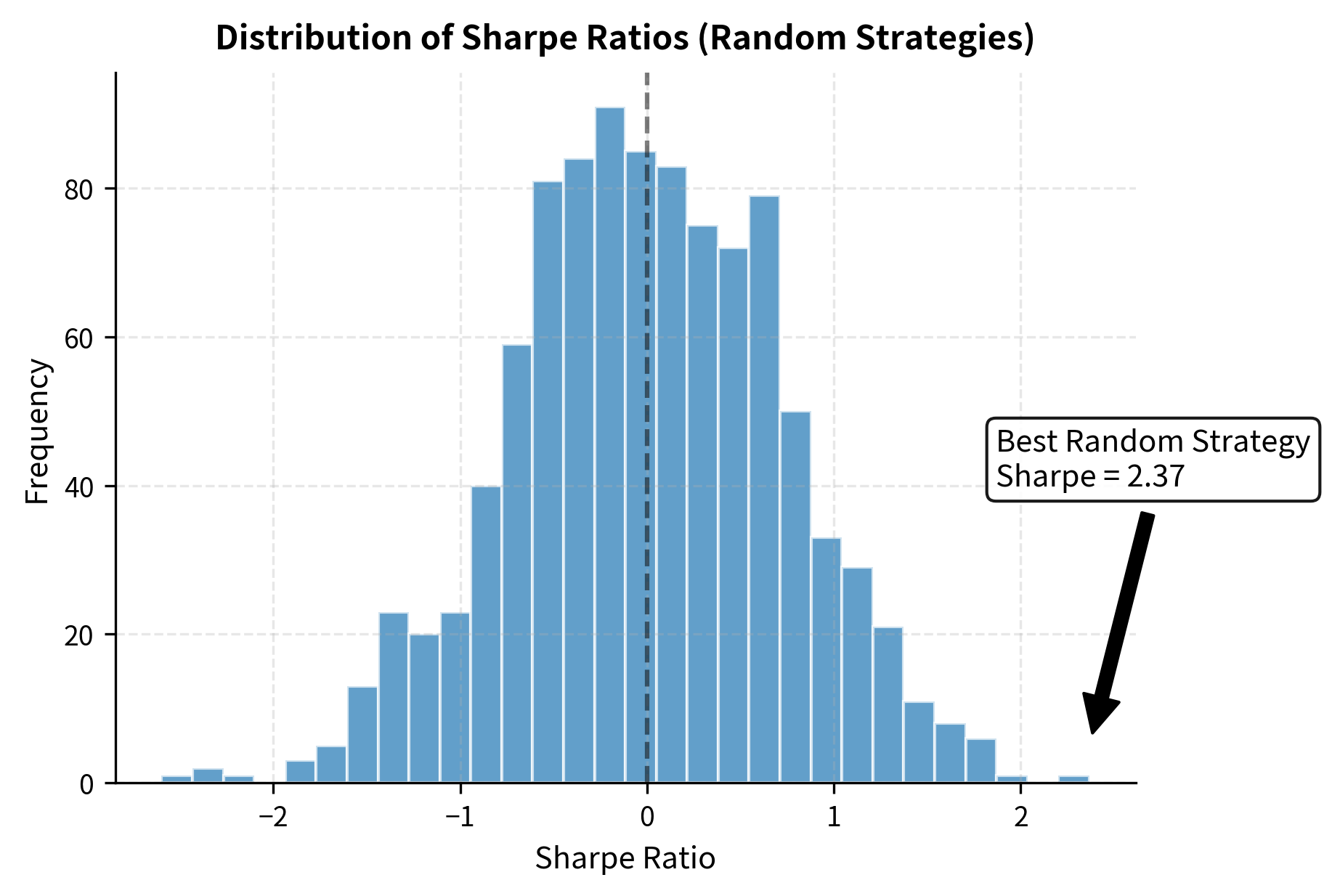
The best of 1000 random strategies shows a Sharpe ratio that would be impressive for a real strategy, but it has no predictive power whatsoever. The random strategy that happened to align with the market's movements during this particular period looks skilled, but this apparent skill is entirely illusory. This demonstration illustrates why we must account for the number of strategies tested when evaluating results, and why out-of-sample validation is so critical. A strategy that survives rigorous out-of-sample testing is much more likely to have genuine predictive power than one selected purely based on in-sample performance.

Other Common BiasesLink Copied

Several additional biases can corrupt backtest results and lead to overoptimistic assessments of strategy performance. Being aware of these pitfalls helps you design more robust simulations and interpret results more critically.

Additional biases include:

Transaction cost neglect: Ignoring costs can turn a profitable strategy into a losing one. High-turnover strategies are particularly vulnerable to the cumulative drag of commissions and spreads.
Market impact neglect: Assuming unlimited liquidity. Large orders often move prices against you, meaning historical closing prices may not be achievable for substantial volumes.
Rebalancing frequency mismatch: Testing at a higher frequency (e.g., daily) than is operationally feasible (e.g., monthly), ignoring execution delays.
Selection bias in time period: Testing only during favorable regimes, such as bull markets, which overstates performance compared to a full market cycle.
Data quality issues: Errors, missing values, or incorrect adjustments can produce spurious signals and persistent bias.

As we'll explore in the next chapter on transaction costs and market impact, realistic friction modeling can reduce apparent strategy returns by 50% or more for active strategies. This makes cost modeling one of the most important aspects of realistic backtesting.

Performance MetricsLink Copied

Once you've run a bias-free backtest, you need metrics to evaluate the results and understand the risk-return characteristics of your strategy. As we discussed in Part IV on portfolio performance measurement, returns alone are insufficient for making informed decisions. We need risk-adjusted measures that account for the volatility and drawdowns incurred to achieve those returns. A strategy that earns 20% annual returns with 10% volatility is quite different from one that earns 20% with 40% volatility, even though the raw returns are identical.

Return MetricsLink Copied

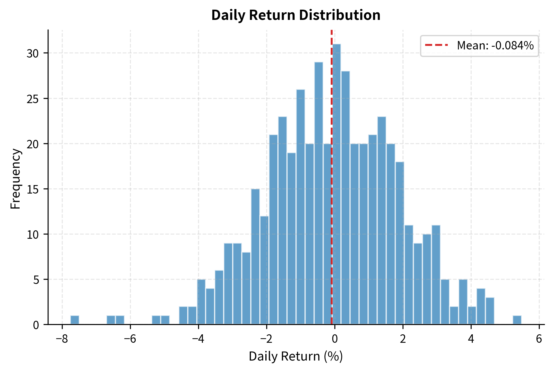
The foundation of performance measurement is the return series, which captures how the portfolio's value changed over time. From the simulated portfolio values, we compute various return statistics that describe the strategy's profitability and growth characteristics.

In[15]:

Code

def calculate_return_metrics(portfolio_values):
    """
    Calculate basic return metrics from a portfolio value series.
    """
    # Convert to pandas if needed
    if isinstance(portfolio_values, np.ndarray):
        portfolio_values = pd.Series(portfolio_values)

    # Simple returns
    returns = portfolio_values.pct_change().dropna()

    # Total return
    total_return = portfolio_values.iloc[-1] / portfolio_values.iloc[0] - 1

    # Annualized return (assuming 252 trading days)
    n_years = len(returns) / 252
    annualized_return = (1 + total_return) ** (1 / n_years) - 1

    # Annualized volatility
    annualized_vol = returns.std() * np.sqrt(252)

    return {
        "total_return": total_return,
        "annualized_return": annualized_return,
        "annualized_volatility": annualized_vol,
        "daily_returns": returns,
    }

def calculate_return_metrics(portfolio_values):
    """
    Calculate basic return metrics from a portfolio value series.
    """
    # Convert to pandas if needed
    if isinstance(portfolio_values, np.ndarray):
        portfolio_values = pd.Series(portfolio_values)

    # Simple returns
    returns = portfolio_values.pct_change().dropna()

    # Total return
    total_return = portfolio_values.iloc[-1] / portfolio_values.iloc[0] - 1

    # Annualized return (assuming 252 trading days)
    n_years = len(returns) / 252
    annualized_return = (1 + total_return) ** (1 / n_years) - 1

    # Annualized volatility
    annualized_vol = returns.std() * np.sqrt(252)

    return {
        "total_return": total_return,
        "annualized_return": annualized_return,
        "annualized_volatility": annualized_vol,
        "daily_returns": returns,
    }

The Sharpe Ratio and Its VariantsLink Copied

The Sharpe ratio, covered extensively in Part IV, remains the dominant risk-adjusted performance measure in quantitative finance. It normalizes returns against risk, allowing for fair comparison between strategies with different volatility profiles. The fundamental insight behind the Sharpe ratio is that returns should be evaluated relative to the risk taken to achieve them. A high-return, high-risk strategy may be less attractive than a moderate-return, low-risk strategy when viewed through this lens.

The Sharpe ratio expresses excess return per unit of volatility, providing a standardized measure of risk-adjusted performance:

\text{Sharpe Ratio} = \frac{R_p - R_f}{\sigma_p}

To understand this formula, let's examine each component. The term $R_p$ represents the annualized portfolio return, measuring how much the strategy earned over the evaluation period expressed as an annual rate. The term $R_f$ denotes the risk-free interest rate, typically proxied by Treasury bill yields, which represents the return you could have earned without taking any market risk. The difference $R_p - R_f$ is the excess return generated by the strategy over the risk-free alternative, capturing the additional compensation you received for bearing the strategy's risks. Finally, $\sigma_p$ is the annualized standard deviation of portfolio returns, commonly called volatility, which measures the typical magnitude of return fluctuations around the mean.

The Sharpe ratio thus answers a crucial question: how much excess return did the strategy generate for each unit of risk it assumed? A Sharpe ratio of 1.0 means the strategy earned 1% of excess return for every 1% of volatility. Higher values indicate more efficient risk-reward tradeoffs, while negative values indicate the strategy failed to beat the risk-free rate.

In[16]:

Code

def calculate_sharpe_ratio(returns, risk_free_rate=0.02, periods_per_year=252):
    """
    Calculate annualized Sharpe ratio.

    Parameters:
    -----------
    returns : array-like
        Period returns (daily, monthly, etc.)
    risk_free_rate : float
        Annual risk-free rate
    periods_per_year : int
        Number of periods per year (252 for daily, 12 for monthly)
    """
    excess_returns = returns - risk_free_rate / periods_per_year

    if excess_returns.std() == 0:
        return 0

    sharpe = excess_returns.mean() / excess_returns.std()
    annualized_sharpe = sharpe * np.sqrt(periods_per_year)

    return annualized_sharpe

def calculate_sharpe_ratio(returns, risk_free_rate=0.02, periods_per_year=252):
    """
    Calculate annualized Sharpe ratio.

    Parameters:
    -----------
    returns : array-like
        Period returns (daily, monthly, etc.)
    risk_free_rate : float
        Annual risk-free rate
    periods_per_year : int
        Number of periods per year (252 for daily, 12 for monthly)
    """
    excess_returns = returns - risk_free_rate / periods_per_year

    if excess_returns.std() == 0:
        return 0

    sharpe = excess_returns.mean() / excess_returns.std()
    annualized_sharpe = sharpe * np.sqrt(periods_per_year)

    return annualized_sharpe

The Sharpe ratio has important limitations that you should keep in mind when using it to evaluate strategies. It penalizes upside and downside volatility equally, treating a strategy that experiences large gains the same as one that experiences large losses. Additionally, it assumes returns are normally distributed, which may not hold for strategies with fat tails or asymmetric return profiles. Several alternative metrics address these limitations by focusing on specific aspects of risk that the Sharpe ratio overlooks.

Alternative metrics address specific limitations of the Sharpe ratio:

Sortino Ratio: Uses downside deviation (volatility of negative returns) instead of total volatility. This rewards strategies that achieve volatility through upside gains rather than losses.
Calmar Ratio: Divides annualized return by maximum drawdown. This highlights the worst loss experience, which is critical for assessing psychological and capital feasibility.
Information Ratio: Measures excess return relative to a benchmark divided by tracking error, capturing the consistency of outperformance.

In[17]:

Code

def calculate_sortino_ratio(returns, risk_free_rate=0.02, periods_per_year=252):
    """
    Sortino ratio: like Sharpe but using downside deviation only.
    """
    excess_returns = returns - risk_free_rate / periods_per_year

    # Downside returns only
    downside_returns = excess_returns[excess_returns < 0]

    if len(downside_returns) == 0 or downside_returns.std() == 0:
        return np.inf  # No downside

    downside_deviation = downside_returns.std()
    sortino = excess_returns.mean() / downside_deviation

    return sortino * np.sqrt(periods_per_year)

def calculate_sortino_ratio(returns, risk_free_rate=0.02, periods_per_year=252):
    """
    Sortino ratio: like Sharpe but using downside deviation only.
    """
    excess_returns = returns - risk_free_rate / periods_per_year

    # Downside returns only
    downside_returns = excess_returns[excess_returns < 0]

    if len(downside_returns) == 0 or downside_returns.std() == 0:
        return np.inf  # No downside

    downside_deviation = downside_returns.std()
    sortino = excess_returns.mean() / downside_deviation

    return sortino * np.sqrt(periods_per_year)

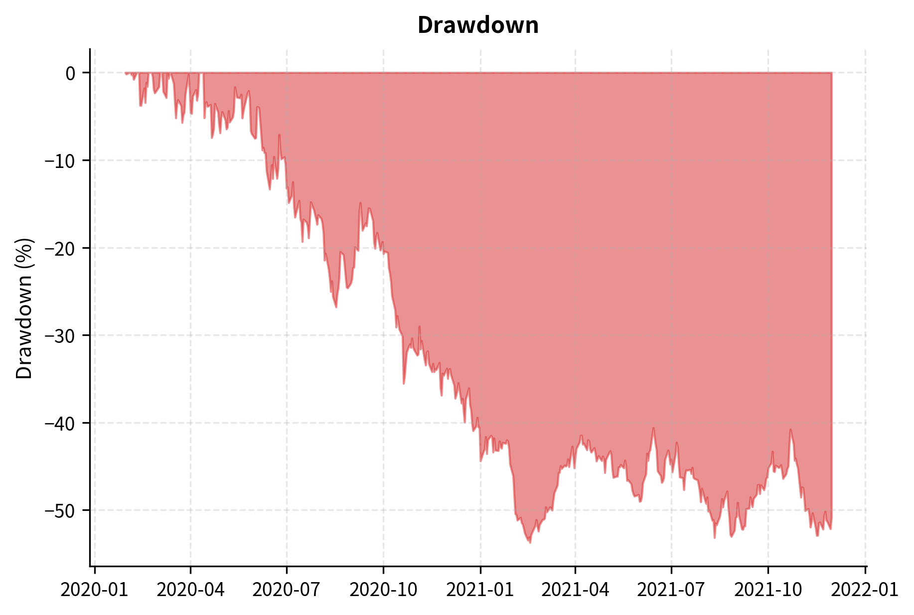
Maximum DrawdownLink Copied

Maximum drawdown measures the largest peak-to-trough decline in portfolio value. It represents the worst loss you would have experienced if you had the misfortune of buying at the top and selling at the bottom during the evaluation period. This metric captures a dimension of risk that volatility-based measures may miss: the severity of the worst period of losses.

To calculate drawdown at any point in time, we first need to establish the high-water mark, which is the highest portfolio value achieved up to that moment. The drawdown is then the percentage decline from that peak:

\text{Drawdown}_t = \frac{V_t - \max_{s \leq t}(V_s)}{\max_{s \leq t}(V_s)}

In this formula, $V_t$ represents the portfolio value at time $t$ , while $\max_{s \leq t}(V_s)$ denotes the high-water mark, which is the highest portfolio value observed up to time $t$ . The numerator $V_t - \max_{s \leq t}(V_s)$ gives the drawdown magnitude, measuring the current loss relative to the running peak. This value is always zero or negative, with more negative values indicating larger declines from the peak.

This formula quantifies the "pain" you experience at any point in time relative to your previous high-water mark. When the portfolio reaches a new high, the drawdown is zero. When the portfolio declines, the drawdown becomes negative, showing how far the portfolio has fallen from its best performance.

The maximum drawdown measures the worst loss over the entire evaluation period by finding the minimum, that is, the most negative, value in the drawdown series:

\text{Max Drawdown} = \min_t(\text{Drawdown}_t)

Here, $\text{Drawdown}_t$ is the percentage decline calculated at each time step $t$ , and the $\min_t$ operator selects the most negative value from the entire series, representing the deepest trough reached during the evaluation period.

In[18]:

Code

def calculate_drawdowns(portfolio_values):
    """
    Calculate drawdown series and maximum drawdown.
    """
    # Running maximum
    running_max = portfolio_values.cummax()

    # Drawdown at each point
    drawdowns = (portfolio_values - running_max) / running_max

    # Maximum drawdown
    max_drawdown = drawdowns.min()

    # Find the dates of the max drawdown
    max_dd_end = drawdowns.idxmin()
    max_dd_start = portfolio_values[:max_dd_end].idxmax()

    return {
        "drawdowns": drawdowns,
        "max_drawdown": max_drawdown,
        "max_dd_start": max_dd_start,
        "max_dd_end": max_dd_end,
    }

def calculate_drawdowns(portfolio_values):
    """
    Calculate drawdown series and maximum drawdown.
    """
    # Running maximum
    running_max = portfolio_values.cummax()

    # Drawdown at each point
    drawdowns = (portfolio_values - running_max) / running_max

    # Maximum drawdown
    max_drawdown = drawdowns.min()

    # Find the dates of the max drawdown
    max_dd_end = drawdowns.idxmin()
    max_dd_start = portfolio_values[:max_dd_end].idxmax()

    return {
        "drawdowns": drawdowns,
        "max_drawdown": max_drawdown,
        "max_dd_start": max_dd_start,
        "max_dd_end": max_dd_end,
    }

Maximum drawdown is particularly important because it relates directly to investor psychology and practical capital requirements. A strategy might have excellent risk-adjusted returns on paper but require holding through a 50% loss, which few investors can tolerate psychologically or financially. Many investors will abandon a strategy during a large drawdown, realizing losses at the worst possible time. Understanding the maximum drawdown helps set realistic expectations and determine appropriate position sizing.

Win Rate and Profit FactorLink Copied

Beyond volatility-based metrics, traders often examine win/loss statistics that describe the distribution of individual trading outcomes. These metrics provide intuition about how the strategy generates its returns and can help identify potential problems.

In[19]:

Code

def calculate_trade_statistics(returns):
    """
    Calculate win rate, profit factor, and related statistics.
    """
    winning_periods = returns[returns > 0]
    losing_periods = returns[returns < 0]

    win_rate = len(winning_periods) / len(returns)

    # Average win vs average loss
    avg_win = winning_periods.mean() if len(winning_periods) > 0 else 0
    avg_loss = abs(losing_periods.mean()) if len(losing_periods) > 0 else 0

    # Profit factor: gross profits / gross losses
    gross_profit = winning_periods.sum()
    gross_loss = abs(losing_periods.sum())
    profit_factor = gross_profit / gross_loss if gross_loss > 0 else np.inf

    # Expectancy: average profit per trade
    expectancy = returns.mean()

    return {
        "win_rate": win_rate,
        "avg_win": avg_win,
        "avg_loss": avg_loss,
        "profit_factor": profit_factor,
        "expectancy": expectancy,
    }

def calculate_trade_statistics(returns):
    """
    Calculate win rate, profit factor, and related statistics.
    """
    winning_periods = returns[returns > 0]
    losing_periods = returns[returns < 0]

    win_rate = len(winning_periods) / len(returns)

    # Average win vs average loss
    avg_win = winning_periods.mean() if len(winning_periods) > 0 else 0
    avg_loss = abs(losing_periods.mean()) if len(losing_periods) > 0 else 0

    # Profit factor: gross profits / gross losses
    gross_profit = winning_periods.sum()
    gross_loss = abs(losing_periods.sum())
    profit_factor = gross_profit / gross_loss if gross_loss > 0 else np.inf

    # Expectancy: average profit per trade
    expectancy = returns.mean()

    return {
        "win_rate": win_rate,
        "avg_win": avg_win,
        "avg_loss": avg_loss,
        "profit_factor": profit_factor,
        "expectancy": expectancy,
    }

Comprehensive Performance ReportLink Copied

Let's combine these metrics into a comprehensive performance analysis that provides a complete picture of strategy behavior:

In[20]:

Code

def run_momentum_backtest(prices, lookback=20):
    """
    Run a momentum strategy backtest and return portfolio values.
    """
    returns = prices.pct_change()

    # Momentum signal based on past returns
    # shift(1) ensures signal at t uses data up to t-1
    momentum = returns.rolling(window=lookback).mean().shift(1)

    # Position: +1 when momentum positive, -1 when negative
    position = np.sign(momentum)

    # Strategy returns: position * returns
    strategy_returns = position * returns
    strategy_returns = strategy_returns.dropna()

    # Convert to portfolio values
    portfolio_values = 100000 * (1 + strategy_returns).cumprod()

    return portfolio_values, strategy_returns


# Run backtest on Stock A
portfolio_values, strategy_returns = run_momentum_backtest(prices_df["Stock_A"])

def run_momentum_backtest(prices, lookback=20):
    """
    Run a momentum strategy backtest and return portfolio values.
    """
    returns = prices.pct_change()

    # Momentum signal based on past returns
    # shift(1) ensures signal at t uses data up to t-1
    momentum = returns.rolling(window=lookback).mean().shift(1)

    # Position: +1 when momentum positive, -1 when negative
    position = np.sign(momentum)

    # Strategy returns: position * returns
    strategy_returns = position * returns
    strategy_returns = strategy_returns.dropna()

    # Convert to portfolio values
    portfolio_values = 100000 * (1 + strategy_returns).cumprod()

    return portfolio_values, strategy_returns


# Run backtest on Stock A
portfolio_values, strategy_returns = run_momentum_backtest(prices_df["Stock_A"])

In[21]:

Code

def generate_performance_report(
    portfolio_values, strategy_returns, strategy_name="Strategy"
):
    """
    Generate a comprehensive performance report.
    """
    returns_metrics = calculate_return_metrics(portfolio_values)
    drawdown_metrics = calculate_drawdowns(portfolio_values)
    trade_stats = calculate_trade_statistics(strategy_returns)

    sharpe = calculate_sharpe_ratio(strategy_returns)
    sortino = calculate_sortino_ratio(strategy_returns)
    calmar = (
        returns_metrics["annualized_return"]
        / abs(drawdown_metrics["max_drawdown"])
        if drawdown_metrics["max_drawdown"] != 0
        else np.inf
    )

    report = {
        "Strategy": strategy_name,
        "Total Return": f"{returns_metrics['total_return'] * 100:.2f}%",
        "Annualized Return": f"{returns_metrics['annualized_return'] * 100:.2f}%",
        "Annualized Volatility": f"{returns_metrics['annualized_volatility'] * 100:.2f}%",
        "Sharpe Ratio": f"{sharpe:.2f}",
        "Sortino Ratio": f"{sortino:.2f}",
        "Calmar Ratio": f"{calmar:.2f}",
        "Maximum Drawdown": f"{drawdown_metrics['max_drawdown'] * 100:.2f}%",
        "Win Rate": f"{trade_stats['win_rate'] * 100:.1f}%",
        "Profit Factor": f"{trade_stats['profit_factor']:.2f}",
    }

    return report


report = generate_performance_report(
    portfolio_values, strategy_returns, "Momentum"
)

def generate_performance_report(
    portfolio_values, strategy_returns, strategy_name="Strategy"
):
    """
    Generate a comprehensive performance report.
    """
    returns_metrics = calculate_return_metrics(portfolio_values)
    drawdown_metrics = calculate_drawdowns(portfolio_values)
    trade_stats = calculate_trade_statistics(strategy_returns)

    sharpe = calculate_sharpe_ratio(strategy_returns)
    sortino = calculate_sortino_ratio(strategy_returns)
    calmar = (
        returns_metrics["annualized_return"]
        / abs(drawdown_metrics["max_drawdown"])
        if drawdown_metrics["max_drawdown"] != 0
        else np.inf
    )

    report = {
        "Strategy": strategy_name,
        "Total Return": f"{returns_metrics['total_return'] * 100:.2f}%",
        "Annualized Return": f"{returns_metrics['annualized_return'] * 100:.2f}%",
        "Annualized Volatility": f"{returns_metrics['annualized_volatility'] * 100:.2f}%",
        "Sharpe Ratio": f"{sharpe:.2f}",
        "Sortino Ratio": f"{sortino:.2f}",
        "Calmar Ratio": f"{calmar:.2f}",
        "Maximum Drawdown": f"{drawdown_metrics['max_drawdown'] * 100:.2f}%",
        "Win Rate": f"{trade_stats['win_rate'] * 100:.1f}%",
        "Profit Factor": f"{trade_stats['profit_factor']:.2f}",
    }

    return report


report = generate_performance_report(
    portfolio_values, strategy_returns, "Momentum"
)

Out[22]:

Console

==================================================
BACKTEST PERFORMANCE REPORT
==================================================
Strategy...................... Momentum
Total Return.................. -39.21%
Annualized Return............. -23.08%
Annualized Volatility......... 31.18%
Sharpe Ratio.................. -0.74
Sortino Ratio................. -1.17
Calmar Ratio.................. -0.43
Maximum Drawdown.............. -53.74%
Win Rate...................... 48.6%
Profit Factor................. 0.90
==================================================

The performance report quantifies the strategy's risk-return profile through multiple lenses. Metrics like the Sharpe ratio, which measures excess return per unit of risk, and maximum drawdown, which captures the worst peak-to-trough decline, provide a more complete picture than total return alone. By examining these metrics together, you can assess whether the strategy's returns are commensurate with the risks it takes and whether those risks are acceptable for your investment objectives.

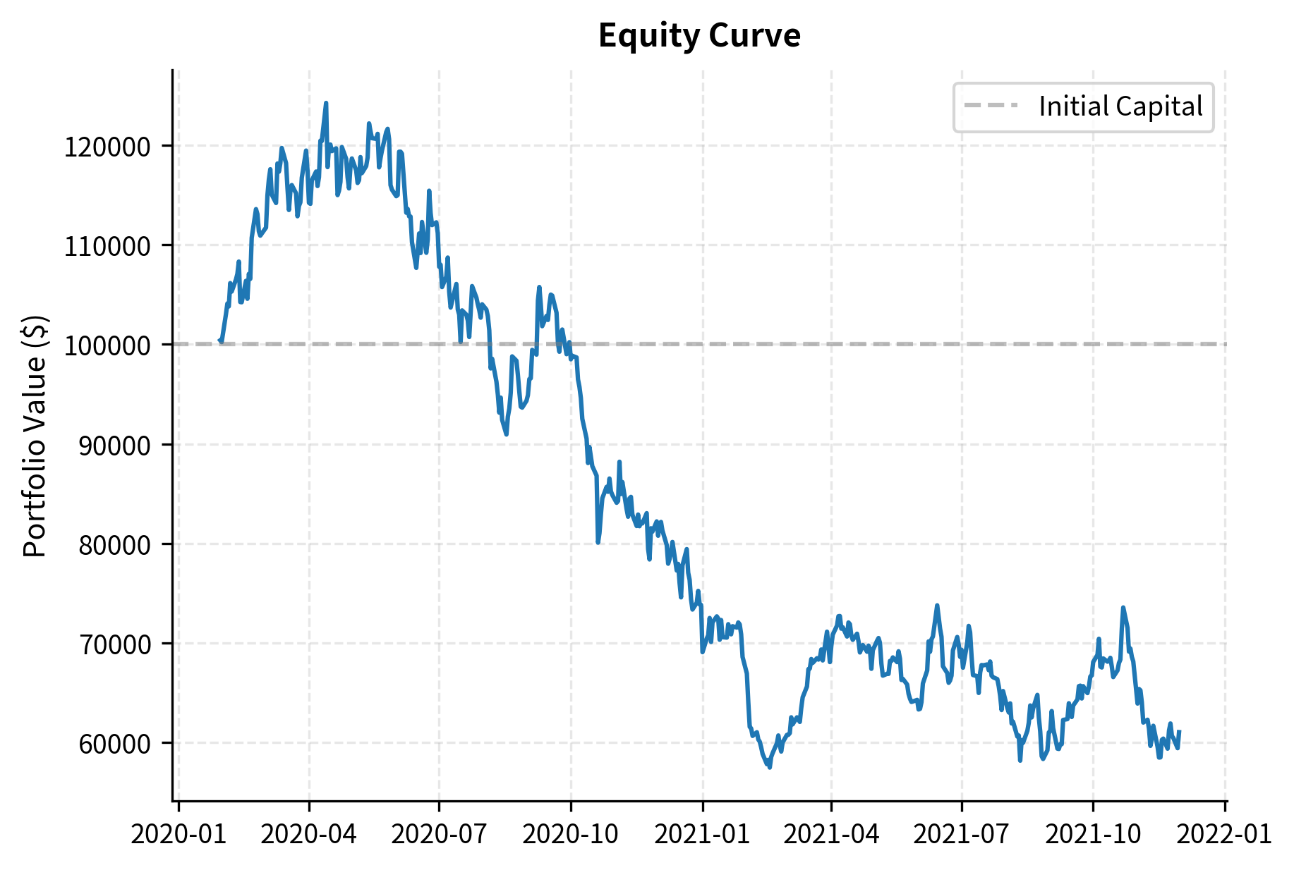
Visualizing PerformanceLink Copied

Visual analysis complements numerical metrics by revealing patterns in strategy behavior over time. While summary statistics condense performance into single numbers, charts show how that performance unfolded, making it easier to identify regime changes, unusual periods, and potential concerns.

Out[23]:

Visualization

Momentum strategy equity curve showing portfolio value growth over time. The portfolio grows from $100,000 to approximately $120,000, reflecting the cumulative impact of the strategy's trading decisions.

Out[24]:

Visualization

Momentum strategy drawdown profile over the backtest period. The chart displays the percentage decline from the running high-water mark, highlighting the risk profile and recovery periods.

Out[25]:

Visualization

Distribution of daily returns for the momentum strategy. The histogram reveals the frequency of return magnitudes, showing the central tendency and the presence of any fat tails.

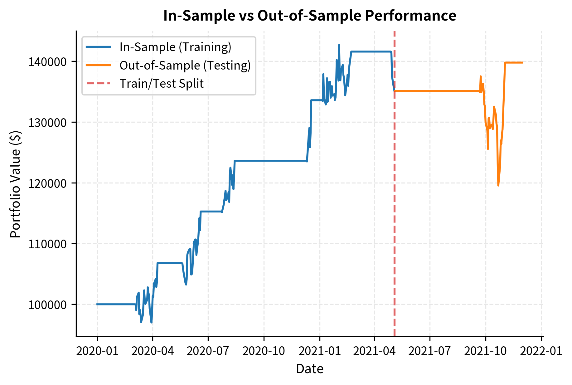
Out-of-Sample Testing and ValidationLink Copied

In-sample performance, which measures how a strategy did on the data used to develop it, tells us almost nothing about future performance. This is a counterintuitive but critical insight: the strategy was designed to perform well on that specific data, so finding that it does perform well provides little evidence of genuine predictive power. The true test of a strategy is out-of-sample evaluation, which assesses how it performs on data it has never seen. Only out-of-sample results can distinguish between strategies that have discovered real patterns and those that have merely memorized historical noise.

Train-Test SplitLink Copied

The simplest validation approach divides data into training and testing periods. The training period is used to develop and tune the strategy, while the testing period is held out for final evaluation. This mirrors how the strategy would actually be deployed: you develop it on historical data and then trade it going forward on new, unseen data.

In[26]:

Code

def train_test_split_backtest(prices, train_fraction=0.7):
    """
    Split data into training and testing periods.

    Training period: develop and tune strategy parameters
    Testing period: evaluate final performance (no tuning allowed)
    """
    split_idx = int(len(prices) * train_fraction)

    train_data = prices.iloc[:split_idx]
    test_data = prices.iloc[split_idx:]

    return train_data, test_data


train_prices, test_prices = train_test_split_backtest(prices_df["Stock_A"])

def train_test_split_backtest(prices, train_fraction=0.7):
    """
    Split data into training and testing periods.

    Training period: develop and tune strategy parameters
    Testing period: evaluate final performance (no tuning allowed)
    """
    split_idx = int(len(prices) * train_fraction)

    train_data = prices.iloc[:split_idx]
    test_data = prices.iloc[split_idx:]

    return train_data, test_data


train_prices, test_prices = train_test_split_backtest(prices_df["Stock_A"])

Out[27]:

Console

Training period: 2020-01-01 to 2021-05-04
Testing period:  2021-05-05 to 2021-11-30
Training days: 350, Testing days: 150

The critical rule of out-of-sample testing is that you may only test on the held-out data once. If you test, don't like the results, modify your strategy, and test again, you've converted your test set into a training set. The strategy is now implicitly optimized to the "out-of-sample" data, because your modifications were guided by feedback from that data. This contamination is insidious because it's easy to rationalize each modification as a reasonable improvement, but the cumulative effect is to fit the test data just as thoroughly as the original training data.

Walk-Forward AnalysisLink Copied

Walk-forward analysis extends the train-test concept by repeatedly retraining the strategy as new data becomes available. This approach better simulates real-world conditions where strategies are periodically updated to adapt to changing market conditions. Rather than training once and testing once, walk-forward analysis creates a sequence of train-test cycles that together span the entire evaluation period.

The process works as follows: first, train the strategy on an initial window of data and select the best parameters. Then, apply those parameters to the subsequent testing window and record the out-of-sample results. Next, roll the windows forward, incorporating the previous test data into the new training set. Repeat this process until you've walked through the entire dataset. The final performance is measured by combining all the out-of-sample testing periods.

In[28]:

Code

def walk_forward_backtest(
    prices, train_window=200, test_window=50, lookback_range=(10, 30)
):
    """
    Walk-forward analysis: train, test, roll forward, repeat.

    Parameters:
    -----------
    prices : pd.Series
        Price series
    train_window : int
        Days to use for training
    test_window : int
        Days to test before retraining
    lookback_range : tuple
        Range of momentum lookbacks to optimize over
    """
    all_test_returns = []
    optimization_history = []

    start_idx = train_window

    while start_idx + test_window <= len(prices):
        # Training data: preceding train_window days
        train_data = prices.iloc[start_idx - train_window : start_idx]

        # Test data: next test_window days
        test_end = min(start_idx + test_window, len(prices))
        test_data = prices.iloc[start_idx:test_end]

        # Optimize lookback on training data
        best_lookback = None
        best_sharpe = -np.inf

        for lookback in range(lookback_range[0], lookback_range[1] + 1):
            train_pv, train_ret = run_momentum_backtest(
                train_data, lookback=lookback
            )
            if len(train_ret) > 0:
                sharpe = calculate_sharpe_ratio(train_ret)
                if sharpe > best_sharpe:
                    best_sharpe = sharpe
                    best_lookback = lookback

        # Apply optimized parameter to test period
        if best_lookback is not None:
            _, test_returns = run_momentum_backtest(
                prices.iloc[start_idx - best_lookback : test_end],
                lookback=best_lookback,
            )
            # Only keep returns from actual test period
            test_returns = test_returns.iloc[-len(test_data) :]
            all_test_returns.append(test_returns)

            optimization_history.append(
                {
                    "train_end": prices.index[start_idx - 1],
                    "test_start": prices.index[start_idx],
                    "best_lookback": best_lookback,
                    "train_sharpe": best_sharpe,
                }
            )

        # Roll forward
        start_idx += test_window

    # Combine all test period returns
    combined_returns = pd.concat(all_test_returns)

    return combined_returns, optimization_history


wf_returns, wf_history = walk_forward_backtest(prices_df["Stock_A"])

def walk_forward_backtest(
    prices, train_window=200, test_window=50, lookback_range=(10, 30)
):
    """
    Walk-forward analysis: train, test, roll forward, repeat.

    Parameters:
    -----------
    prices : pd.Series
        Price series
    train_window : int
        Days to use for training
    test_window : int
        Days to test before retraining
    lookback_range : tuple
        Range of momentum lookbacks to optimize over
    """
    all_test_returns = []
    optimization_history = []

    start_idx = train_window

    while start_idx + test_window <= len(prices):
        # Training data: preceding train_window days
        train_data = prices.iloc[start_idx - train_window : start_idx]

        # Test data: next test_window days
        test_end = min(start_idx + test_window, len(prices))
        test_data = prices.iloc[start_idx:test_end]

        # Optimize lookback on training data
        best_lookback = None
        best_sharpe = -np.inf

        for lookback in range(lookback_range[0], lookback_range[1] + 1):
            train_pv, train_ret = run_momentum_backtest(
                train_data, lookback=lookback
            )
            if len(train_ret) > 0:
                sharpe = calculate_sharpe_ratio(train_ret)
                if sharpe > best_sharpe:
                    best_sharpe = sharpe
                    best_lookback = lookback

        # Apply optimized parameter to test period
        if best_lookback is not None:
            _, test_returns = run_momentum_backtest(
                prices.iloc[start_idx - best_lookback : test_end],
                lookback=best_lookback,
            )
            # Only keep returns from actual test period
            test_returns = test_returns.iloc[-len(test_data) :]
            all_test_returns.append(test_returns)

            optimization_history.append(
                {
                    "train_end": prices.index[start_idx - 1],
                    "test_start": prices.index[start_idx],
                    "best_lookback": best_lookback,
                    "train_sharpe": best_sharpe,
                }
            )

        # Roll forward
        start_idx += test_window

    # Combine all test period returns
    combined_returns = pd.concat(all_test_returns)

    return combined_returns, optimization_history


wf_returns, wf_history = walk_forward_backtest(prices_df["Stock_A"])

Out[29]:

Console

Walk-Forward Analysis Results:
  Total out-of-sample trading days: 294
  Number of reoptimization periods: 6

Out-of-sample Sharpe ratio: -0.45

Optimization history (first 3 windows):
  Window 1: Lookback=16, Train Sharpe=0.81
  Window 2: Lookback=16, Train Sharpe=0.33
  Window 3: Lookback=30, Train Sharpe=0.29

Walk-forward analysis reveals whether a strategy's edge persists when parameters are updated over time. It also shows parameter stability: if the optimal lookback swings wildly between windows, the strategy may be fitting noise rather than capturing a stable relationship. Stable parameters that change gradually over time suggest a more robust underlying pattern, while erratic parameter changes indicate that the optimization is chasing random fluctuations in the training data.

Cross-Validation for Strategy DevelopmentLink Copied

When developing new strategies, k-fold cross-validation can provide more robust estimates of out-of-sample performance by averaging results across multiple train-test splits. However, standard cross-validation ignores the time-series nature of financial data, where random shuffling would create look-ahead bias by mixing future observations into the training set.

Time-series cross-validation respects temporal ordering by always training on earlier data and testing on later data. This ensures that each test fold uses only information that would have been available at the time of trading. The training window typically expands over time, incorporating more historical data as it becomes available.

In[30]:

Code

def time_series_cv(prices, n_splits=5, min_train_size=100):
    """
    Time-series cross-validation with expanding training window.
    """
    n = len(prices)
    test_size = (n - min_train_size) // n_splits

    splits = []

    for i in range(n_splits):
        train_end = min_train_size + i * test_size
        test_end = train_end + test_size

        if test_end > n:
            break

        train_idx = list(range(train_end))
        test_idx = list(range(train_end, test_end))

        splits.append((train_idx, test_idx))

    return splits


# Demonstrate the splits
cv_splits = time_series_cv(prices_df["Stock_A"], n_splits=5)

def time_series_cv(prices, n_splits=5, min_train_size=100):
    """
    Time-series cross-validation with expanding training window.
    """
    n = len(prices)
    test_size = (n - min_train_size) // n_splits

    splits = []

    for i in range(n_splits):
        train_end = min_train_size + i * test_size
        test_end = train_end + test_size

        if test_end > n:
            break

        train_idx = list(range(train_end))
        test_idx = list(range(train_end, test_end))

        splits.append((train_idx, test_idx))

    return splits


# Demonstrate the splits
cv_splits = time_series_cv(prices_df["Stock_A"], n_splits=5)

Out[31]:

Console

Time Series Cross-Validation Splits:
  Fold 1: Train 2020-01-01 to 2020-05-19 | Test 2020-05-20 to 2020-09-08
  Fold 2: Train 2020-01-01 to 2020-09-08 | Test 2020-09-09 to 2020-12-29
  Fold 3: Train 2020-01-01 to 2020-12-29 | Test 2020-12-30 to 2021-04-20
  Fold 4: Train 2020-01-01 to 2021-04-20 | Test 2021-04-21 to 2021-08-10
  Fold 5: Train 2020-01-01 to 2021-08-10 | Test 2021-08-11 to 2021-11-30

Out[32]:

Visualization

Schematic of expanding window cross-validation splits. The training window (blue) expands over time to include more data, while the testing window (orange) moves forward, preserving the temporal order required for valid backtesting.

The expanding window cross-validation creates multiple test sets while respecting the time order. Notice that each training set ends before its corresponding test set begins, and that the training sets grow larger over time. This approach allows us to evaluate how the strategy would have performed across different market conditions without using future data. By averaging performance across all folds, we get a more stable estimate of out-of-sample performance than a single train-test split would provide.

Statistical Significance TestingLink Copied

Even with proper out-of-sample testing, observed performance could arise from luck rather than skill. A strategy might show positive returns in the test period purely by chance, especially if the test period is short or the returns are highly variable. Statistical tests help quantify this uncertainty by estimating the probability that the observed results could have occurred under the assumption that the strategy has no genuine predictive power.

The null hypothesis is typically that the strategy has zero expected return, meaning no skill. We compute the t-statistic to measure how many standard errors the observed mean return is away from zero:

t = \frac{\bar{r}}{\sigma_r / \sqrt{n}}

This formula tells us how unusual the observed returns are under the null hypothesis of no skill. The term $\bar{r}$ is the mean periodic return of the strategy, representing the average profit or loss per period. The term $\sigma_r$ denotes the standard deviation of returns, capturing the typical variability in performance from period to period. The term $n$ represents the total number of observations, which determines how precisely we can estimate the true mean. The denominator $\sigma_r / \sqrt{n}$ is the standard error of the mean, representing our uncertainty about the true expected return given the observed data. Finally, $t$ is the number of standard errors the mean is away from zero, the null hypothesis value.

A large positive t-statistic suggests the strategy's returns are unlikely to have arisen by chance. We can convert this to a p-value that represents the probability of observing such extreme results if the strategy truly had no edge.

In[33]:

Code

from scipy import stats


def test_strategy_significance(returns, null_return=0):
    """
    Test if strategy returns are significantly different from null hypothesis.
    """
    n = len(returns)
    mean_return = returns.mean()
    std_return = returns.std()

    # T-statistic
    t_stat = (mean_return - null_return) / (std_return / np.sqrt(n))

    # P-value (two-tailed)
    p_value = 2 * (1 - stats.t.cdf(abs(t_stat), df=n - 1))

    # Confidence interval for mean return
    ci_95 = stats.t.interval(
        0.95, df=n - 1, loc=mean_return, scale=std_return / np.sqrt(n)
    )

    return {
        "t_statistic": t_stat,
        "p_value": p_value,
        "confidence_interval_95": ci_95,
        "annualized_mean": mean_return * 252,
        "annualized_ci": (ci_95[0] * 252, ci_95[1] * 252),
    }


significance = test_strategy_significance(strategy_returns)

from scipy import stats


def test_strategy_significance(returns, null_return=0):
    """
    Test if strategy returns are significantly different from null hypothesis.
    """
    n = len(returns)
    mean_return = returns.mean()
    std_return = returns.std()

    # T-statistic
    t_stat = (mean_return - null_return) / (std_return / np.sqrt(n))

    # P-value (two-tailed)
    p_value = 2 * (1 - stats.t.cdf(abs(t_stat), df=n - 1))

    # Confidence interval for mean return
    ci_95 = stats.t.interval(
        0.95, df=n - 1, loc=mean_return, scale=std_return / np.sqrt(n)
    )

    return {
        "t_statistic": t_stat,
        "p_value": p_value,
        "confidence_interval_95": ci_95,
        "annualized_mean": mean_return * 252,
        "annualized_ci": (ci_95[0] * 252, ci_95[1] * 252),
    }


significance = test_strategy_significance(strategy_returns)

Out[34]:

Console

Statistical Significance Test:
  T-statistic: -0.934
  P-value: 0.3506
  95% CI for annualized return: (-65.49%, 23.28%)

  Result: Cannot reject null hypothesis of zero returns

A low p-value, typically below 0.05, suggests the strategy's returns are unlikely to result from chance alone. However, remember to adjust for multiple testing if you've evaluated many strategies. Methods like the Bonferroni correction or false discovery rate (FDR) control, which we covered in Part I on statistical inference, become essential when you've tested dozens or hundreds of strategy variants. Without such adjustments, the probability of finding at least one spuriously significant result grows rapidly with the number of tests conducted.

Building a Complete BacktestLink Copied

Let's bring together all the concepts into a complete, realistic backtest implementation. We'll test a simple mean-reversion strategy while carefully avoiding biases and applying proper validation. This comprehensive example demonstrates how the individual components combine into a coherent backtesting workflow.

Strategy DefinitionLink Copied

Our strategy will trade based on Bollinger Bands, a mean-reversion approach where we buy when price falls below the lower band and sell when it rises above the upper band. The economic intuition is that prices tend to revert to their recent average, so extreme deviations represent temporary mispricings that will correct. When the price falls significantly below its moving average, the asset is potentially oversold and likely to bounce back. When the price rises significantly above its moving average, the asset is potentially overbought and likely to pull back.

In[35]:

Code

class BollingerBandStrategy:
    """
    Mean-reversion strategy using Bollinger Bands.

    Buy signal: price closes below lower band (oversold)
    Sell signal: price closes above upper band (overbought)
    """

    def __init__(self, lookback=20, num_std=2):
        self.lookback = lookback
        self.num_std = num_std

    def generate_signals(self, prices):
        """Generate trading signals from price data."""
        # Calculate bands using only past data
        rolling_mean = prices.rolling(window=self.lookback).mean()
        rolling_std = prices.rolling(window=self.lookback).std()

        upper_band = rolling_mean + self.num_std * rolling_std
        lower_band = rolling_mean - self.num_std * rolling_std

        # Shift to avoid look-ahead bias: signal based on yesterday's bands
        upper_band = upper_band.shift(1)
        lower_band = lower_band.shift(1)
        rolling_mean = rolling_mean.shift(1)

        # Generate signals
        # +1: buy (price below lower band)
        # -1: sell (price above upper band)
        # 0: hold (between bands)
        signals = pd.Series(0, index=prices.index)
        signals[prices < lower_band] = 1  # Buy signal
        signals[prices > upper_band] = -1  # Sell signal

        return signals, rolling_mean, upper_band, lower_band

class BollingerBandStrategy:
    """
    Mean-reversion strategy using Bollinger Bands.

    Buy signal: price closes below lower band (oversold)
    Sell signal: price closes above upper band (overbought)
    """

    def __init__(self, lookback=20, num_std=2):
        self.lookback = lookback
        self.num_std = num_std

    def generate_signals(self, prices):
        """Generate trading signals from price data."""
        # Calculate bands using only past data
        rolling_mean = prices.rolling(window=self.lookback).mean()
        rolling_std = prices.rolling(window=self.lookback).std()

        upper_band = rolling_mean + self.num_std * rolling_std
        lower_band = rolling_mean - self.num_std * rolling_std

        # Shift to avoid look-ahead bias: signal based on yesterday's bands
        upper_band = upper_band.shift(1)
        lower_band = lower_band.shift(1)
        rolling_mean = rolling_mean.shift(1)

        # Generate signals
        # +1: buy (price below lower band)
        # -1: sell (price above upper band)
        # 0: hold (between bands)
        signals = pd.Series(0, index=prices.index)
        signals[prices < lower_band] = 1  # Buy signal
        signals[prices > upper_band] = -1  # Sell signal

        return signals, rolling_mean, upper_band, lower_band

Backtest Engine with Transaction CostsLink Copied

We'll incorporate transaction costs to make the simulation more realistic. Transaction costs are a critical component of any serious backtest because they can dramatically affect net profitability, especially for strategies that trade frequently. A strategy that looks highly profitable before costs may become marginal or even unprofitable after accounting for the friction of trading.

In[36]:

Code

class BacktestEngine:
    """
    Event-driven backtest engine with transaction cost modeling.
    """

    def __init__(self, initial_capital=100000, transaction_cost=0.001):
        """
        Parameters:
        -----------
        initial_capital : float
            Starting capital in dollars
        transaction_cost : float
            Transaction cost as fraction of trade value (0.001 = 0.1% = 10bps)
        """
        self.initial_capital = initial_capital
        self.transaction_cost = transaction_cost

    def run(self, prices, signals):
        """
        Execute backtest given prices and signals.

        Returns portfolio values and detailed trade log.
        """
        n = len(prices)

        # Portfolio state
        cash = self.initial_capital
        shares = 0

        # Tracking arrays
        portfolio_values = np.zeros(n)
        positions = np.zeros(n)
        trade_log = []

        for t in range(n):
            current_price = prices.iloc[t]
            current_signal = signals.iloc[t]

            # Execute trades based on signal change
            if t > 0:
                prev_signal = signals.iloc[t - 1]

                # Enter long position
                if current_signal == 1 and shares == 0:
                    # Calculate shares to buy (use all cash minus transaction cost)
                    trade_value = cash / (1 + self.transaction_cost)
                    shares = trade_value / current_price
                    cost = trade_value * self.transaction_cost
                    cash = cash - trade_value - cost

                    trade_log.append(
                        {
                            "date": prices.index[t],
                            "action": "BUY",
                            "shares": shares,
                            "price": current_price,
                            "cost": cost,
                        }
                    )

                # Exit long position
                elif current_signal == -1 and shares > 0:
                    trade_value = shares * current_price
                    cost = trade_value * self.transaction_cost
                    cash = cash + trade_value - cost

                    trade_log.append(
                        {
                            "date": prices.index[t],
                            "action": "SELL",
                            "shares": shares,
                            "price": current_price,
                            "cost": cost,
                        }
                    )

                    shares = 0

            # Record state
            portfolio_values[t] = cash + shares * current_price
            positions[t] = shares

        return pd.Series(portfolio_values, index=prices.index), trade_log


# Run the complete backtest
strategy = BollingerBandStrategy(lookback=20, num_std=2)
signals, ma, upper, lower = strategy.generate_signals(prices_df["Stock_A"])

engine = BacktestEngine(initial_capital=100000, transaction_cost=0.001)
portfolio_values, trades = engine.run(prices_df["Stock_A"], signals)
total_costs = sum(t["cost"] for t in trades)

class BacktestEngine:
    """
    Event-driven backtest engine with transaction cost modeling.
    """

    def __init__(self, initial_capital=100000, transaction_cost=0.001):
        """
        Parameters:
        -----------
        initial_capital : float
            Starting capital in dollars
        transaction_cost : float
            Transaction cost as fraction of trade value (0.001 = 0.1% = 10bps)
        """
        self.initial_capital = initial_capital
        self.transaction_cost = transaction_cost

    def run(self, prices, signals):
        """
        Execute backtest given prices and signals.

        Returns portfolio values and detailed trade log.
        """
        n = len(prices)

        # Portfolio state
        cash = self.initial_capital
        shares = 0

        # Tracking arrays
        portfolio_values = np.zeros(n)
        positions = np.zeros(n)
        trade_log = []

        for t in range(n):
            current_price = prices.iloc[t]
            current_signal = signals.iloc[t]

            # Execute trades based on signal change
            if t > 0:
                prev_signal = signals.iloc[t - 1]

                # Enter long position
                if current_signal == 1 and shares == 0:
                    # Calculate shares to buy (use all cash minus transaction cost)
                    trade_value = cash / (1 + self.transaction_cost)
                    shares = trade_value / current_price
                    cost = trade_value * self.transaction_cost
                    cash = cash - trade_value - cost

                    trade_log.append(
                        {
                            "date": prices.index[t],
                            "action": "BUY",
                            "shares": shares,
                            "price": current_price,
                            "cost": cost,
                        }
                    )

                # Exit long position
                elif current_signal == -1 and shares > 0:
                    trade_value = shares * current_price
                    cost = trade_value * self.transaction_cost
                    cash = cash + trade_value - cost

                    trade_log.append(
                        {
                            "date": prices.index[t],
                            "action": "SELL",
                            "shares": shares,
                            "price": current_price,
                            "cost": cost,
                        }
                    )

                    shares = 0

            # Record state
            portfolio_values[t] = cash + shares * current_price
            positions[t] = shares

        return pd.Series(portfolio_values, index=prices.index), trade_log


# Run the complete backtest
strategy = BollingerBandStrategy(lookback=20, num_std=2)
signals, ma, upper, lower = strategy.generate_signals(prices_df["Stock_A"])

engine = BacktestEngine(initial_capital=100000, transaction_cost=0.001)
portfolio_values, trades = engine.run(prices_df["Stock_A"], signals)
total_costs = sum(t["cost"] for t in trades)

Out[37]:

Console

Backtest completed with 18 trades

Sample trades:
  2020-02-21: BUY  1149.53 shares @ $86.91
  2020-04-06: SELL 1149.53 shares @ $85.86
  2020-05-13: BUY  1182.46 shares @ $83.30
  2020-06-17: SELL 1182.46 shares @ $87.43
  2020-07-24: BUY  1280.39 shares @ $80.58

Total transaction costs paid: $2289.18

The trade log allows us to verify that the strategy executes as intended, buying and selling at the correct signals. Each trade record includes the date, action type, number of shares, execution price, and transaction cost. This detailed logging is essential for debugging and for understanding how the strategy behaves in different market conditions. The total transaction costs figure highlights the friction that will reduce net returns, a critical factor often overlooked in theoretical models that assume frictionless markets.

Comparing In-Sample vs Out-of-Sample PerformanceLink Copied

Finally, let's validate our strategy using proper train-test methodology. We'll optimize the strategy parameters on training data and then evaluate performance on held-out test data to assess how much of the apparent alpha is genuine versus overfit.

In[38]:

Code

def compare_in_out_sample(
    prices,
    strategy_class,
    train_fraction=0.7,
    param_grid={"lookback": [10, 15, 20, 25, 30], "num_std": [1.5, 2.0, 2.5]},
):
    """
    Compare in-sample (optimized) vs out-of-sample performance.
    """
    # Split data
    split_idx = int(len(prices) * train_fraction)
    train_prices = prices.iloc[:split_idx]
    test_prices = prices.iloc[split_idx:]

    # Find best parameters on training data
    best_params = None
    best_in_sample_sharpe = -np.inf

    engine = BacktestEngine(transaction_cost=0.001)

    for lookback in param_grid["lookback"]:
        for num_std in param_grid["num_std"]:
            strategy = strategy_class(lookback=lookback, num_std=num_std)
            signals, _, _, _ = strategy.generate_signals(train_prices)
            pv, _ = engine.run(train_prices, signals)

            returns = pv.pct_change().dropna()
            if len(returns) > 0:
                sharpe = calculate_sharpe_ratio(returns)

                if sharpe > best_in_sample_sharpe:
                    best_in_sample_sharpe = sharpe
                    best_params = {"lookback": lookback, "num_std": num_std}

    # Evaluate best parameters on test data
    best_strategy = strategy_class(**best_params)

    # Re-run on training data with best params
    train_signals, _, _, _ = best_strategy.generate_signals(train_prices)
    train_pv, _ = engine.run(train_prices, train_signals)
    train_returns = train_pv.pct_change().dropna()

    # Run on test data
    test_signals, _, _, _ = best_strategy.generate_signals(test_prices)
    test_pv, _ = engine.run(test_prices, test_signals)
    test_returns = test_pv.pct_change().dropna()

    return {
        "best_params": best_params,
        "in_sample_sharpe": calculate_sharpe_ratio(train_returns),
        "out_of_sample_sharpe": calculate_sharpe_ratio(test_returns),
        "in_sample_return": (train_pv.iloc[-1] / train_pv.iloc[0] - 1) * 100,
        "out_of_sample_return": (test_pv.iloc[-1] / test_pv.iloc[0] - 1) * 100,
        "train_pv": train_pv,
        "test_pv": test_pv,
    }


validation_results = compare_in_out_sample(
    prices_df["Stock_A"], BollingerBandStrategy
)

def compare_in_out_sample(
    prices,
    strategy_class,
    train_fraction=0.7,
    param_grid={"lookback": [10, 15, 20, 25, 30], "num_std": [1.5, 2.0, 2.5]},
):
    """
    Compare in-sample (optimized) vs out-of-sample performance.
    """
    # Split data
    split_idx = int(len(prices) * train_fraction)
    train_prices = prices.iloc[:split_idx]
    test_prices = prices.iloc[split_idx:]

    # Find best parameters on training data
    best_params = None
    best_in_sample_sharpe = -np.inf

    engine = BacktestEngine(transaction_cost=0.001)

    for lookback in param_grid["lookback"]:
        for num_std in param_grid["num_std"]:
            strategy = strategy_class(lookback=lookback, num_std=num_std)
            signals, _, _, _ = strategy.generate_signals(train_prices)
            pv, _ = engine.run(train_prices, signals)

            returns = pv.pct_change().dropna()
            if len(returns) > 0:
                sharpe = calculate_sharpe_ratio(returns)

                if sharpe > best_in_sample_sharpe:
                    best_in_sample_sharpe = sharpe
                    best_params = {"lookback": lookback, "num_std": num_std}

    # Evaluate best parameters on test data
    best_strategy = strategy_class(**best_params)

    # Re-run on training data with best params
    train_signals, _, _, _ = best_strategy.generate_signals(train_prices)
    train_pv, _ = engine.run(train_prices, train_signals)
    train_returns = train_pv.pct_change().dropna()

    # Run on test data
    test_signals, _, _, _ = best_strategy.generate_signals(test_prices)
    test_pv, _ = engine.run(test_prices, test_signals)
    test_returns = test_pv.pct_change().dropna()

    return {
        "best_params": best_params,
        "in_sample_sharpe": calculate_sharpe_ratio(train_returns),
        "out_of_sample_sharpe": calculate_sharpe_ratio(test_returns),
        "in_sample_return": (train_pv.iloc[-1] / train_pv.iloc[0] - 1) * 100,
        "out_of_sample_return": (test_pv.iloc[-1] / test_pv.iloc[0] - 1) * 100,
        "train_pv": train_pv,
        "test_pv": test_pv,
    }


validation_results = compare_in_out_sample(
    prices_df["Stock_A"], BollingerBandStrategy
)

Out[39]:

Console

In-Sample vs Out-of-Sample Validation
==================================================
Best parameters found: {'lookback': 30, 'num_std': 2.0}

In-Sample Performance (training period):
  Sharpe Ratio: 1.29
  Total Return: 35.09%

Out-of-Sample Performance (test period):
  Sharpe Ratio: 0.32
  Total Return: 3.45%

Performance degradation:
  Sharpe drop: 0.97

Out[40]:

Visualization

Line chart showing portfolio equity curves for both training and testing periods with vertical separator. — Comparison of in-sample and out-of-sample performance. The vertical line marks the end of the training period; the strategy continues to profit in the test period but with higher volatility, reflecting realistic performance degradation on unseen data.

The gap between in-sample and out-of-sample performance is typical and expected. This performance degradation, where out-of-sample results are worse than in-sample results, occurs because some of the patterns captured during optimization are noise rather than signal. A strategy that shows similar performance in both periods is more likely to be robust than one where in-sample results far exceed out-of-sample results. When you observe a large gap, it suggests that a significant portion of the apparent alpha was actually overfitting to the training data rather than capturing genuine market inefficiencies that will persist going forward.

Limitations and ImpactLink Copied

Backtesting, despite its importance, has fundamental limitations that you must understand. Recognizing these limitations doesn't mean abandoning backtesting, but rather using it with appropriate humility and supplementing it with other forms of analysis.

Key limitations include:

Testing the past, not the future: Markets evolve and regimes change. Strategies that exploited specific historical conditions (e.g., falling interest rates) may fail as those conditions disappear. Stationarity rarely holds in financial markets.
Data limitations: High-resolution data often has limited history, while long-term data may lack the granularity needed for certain strategies. This necessitates a tradeoff between simulation realism and historical depth.
Execution reality: Simulations often assume trades execute at observed prices without friction. In reality, large orders impact prices. Ignoring market impact can make non-scalable strategies appear profitable.

Despite these limitations, backtesting remains indispensable because it provides the only systematic way to evaluate ideas before risking real capital. The discipline of building a rigorous backtesting framework forces you to formalize your strategy completely, think through data requirements, and establish performance expectations. Strategies that fail in backtests almost certainly fail in live trading; strategies that pass are at least candidates for further testing.

The impact of proper backtesting methodology on quantitative trading has been enormous. The development of walk-forward analysis, cross-validation for financial data, and statistical significance testing for trading strategies has raised the bar for what constitutes evidence of alpha. Techniques for detecting and correcting biases have made it harder for fund managers to present spurious results as genuine skill. The widespread availability of backtesting tools has democratized quantitative trading, allowing individual traders to test ideas that once required institutional resources.

Looking ahead, the next chapters on transaction costs, market microstructure, and execution algorithms will add the remaining pieces needed for realistic strategy evaluation. A complete simulation must account for how you'll actually trade, not just what positions you want to hold.

SummaryLink Copied

This chapter covered the complete workflow for backtesting trading strategies, from building simulation frameworks to validating results statistically. The key takeaways are:

Backtesting architecture requires careful attention to time-series ordering. Whether using event-driven or vectorized approaches, signals must be computed using only past information, and positions must be lagged relative to the data used to generate them.

Biases corrupt backtests in subtle but devastating ways. Look-ahead bias uses future information; survivorship bias excludes failed assets; overfitting finds patterns in noise. Multiple testing across many strategies virtually guarantees finding spuriously profitable results if not properly adjusted.

Performance metrics must be risk-adjusted. The Sharpe ratio remains the standard, but supplementary metrics like maximum drawdown, Sortino ratio, and win rate provide additional perspective. Statistical significance testing quantifies how likely observed performance is to have arisen by chance.

Out-of-sample validation is essential for any serious strategy development. Simple train-test splits provide a first check; walk-forward analysis and time-series cross-validation offer more robust estimates of real-world performance. The gap between in-sample and out-of-sample results reveals how much of apparent alpha is actually overfitting.

Transaction costs matter and must be included even in preliminary backtests. We'll explore sophisticated cost models in the following chapter, but even a simple percentage cost changes which strategies appear viable.

The ultimate purpose of backtesting is not to prove a strategy works but to rigorously test whether it might work. A strategy that survives comprehensive backtesting with realistic assumptions and shows robust out-of-sample performance is a candidate for paper trading and, eventually, live deployment, topics we'll address in later chapters on trading systems and strategy deployment.

QuizLink Copied

Ready to test your understanding? Take this quick quiz to reinforce what you've learned about backtesting and simulation.

Loading component...

Comments

Back to Quantitative Finance

Previous Chapter

Cryptocurrency Markets and Quant Trading

Next Chapter

Transaction Costs & Market Impact: Models & Analysis

Reference

BIBTEXAcademic

@misc{backtestingsimulationframeworksforstrategyvalidation, author = {Michael Brenndoerfer}, title = {Backtesting & Simulation: Frameworks for Strategy Validation}, year = {2026}, url = {https://mbrenndoerfer.com/writing/backtesting-trading-strategies-simulation-frameworks}, organization = {mbrenndoerfer.com}, note = {Accessed: 2025-01-01} }

APAAcademic

Michael Brenndoerfer (2026). Backtesting & Simulation: Frameworks for Strategy Validation. Retrieved from https://mbrenndoerfer.com/writing/backtesting-trading-strategies-simulation-frameworks

MLAAcademic

Michael Brenndoerfer. "Backtesting & Simulation: Frameworks for Strategy Validation." 2026. Web. today. <https://mbrenndoerfer.com/writing/backtesting-trading-strategies-simulation-frameworks>.

CHICAGOAcademic

Michael Brenndoerfer. "Backtesting & Simulation: Frameworks for Strategy Validation." Accessed today. https://mbrenndoerfer.com/writing/backtesting-trading-strategies-simulation-frameworks.

HARVARDAcademic

Michael Brenndoerfer (2026) 'Backtesting & Simulation: Frameworks for Strategy Validation'. Available at: https://mbrenndoerfer.com/writing/backtesting-trading-strategies-simulation-frameworks (Accessed: today).

SimpleBasic

Michael Brenndoerfer (2026). Backtesting & Simulation: Frameworks for Strategy Validation. https://mbrenndoerfer.com/writing/backtesting-trading-strategies-simulation-frameworks

Direct link:

https://mbrenndoerfer.com/writing/backtesting-trading-strategies-simulation-frameworks

About the author: Michael Brenndoerfer

All opinions expressed here are my own and do not reflect the views of my employer.

Michael currently works as an Associate Director of Data Science at EQT Partners in Singapore, leading AI and data initiatives across private capital investments.

With over a decade of experience spanning private equity, management consulting, and software engineering, he specializes in building and scaling analytics capabilities from the ground up. He has published research in leading AI conferences and holds expertise in machine learning, natural language processing, and value creation through data.

View Full Resume Publications Contact Books

Backtesting & Simulation: Frameworks for Strategy Validation

Backtesting and Simulation of Trading StrategiesLink Copied

The Backtesting FrameworkLink Copied

Core ComponentsLink Copied

Event-Driven vs Vectorized BacktestingLink Copied

Data Requirements and AlignmentLink Copied

Biases in BacktestingLink Copied

Look-Ahead BiasLink Copied

Survivorship BiasLink Copied

Overfitting and Data SnoopingLink Copied

Other Common BiasesLink Copied

Performance MetricsLink Copied

Return MetricsLink Copied

The Sharpe Ratio and Its VariantsLink Copied

Maximum DrawdownLink Copied

Win Rate and Profit FactorLink Copied

Comprehensive Performance ReportLink Copied

Visualizing PerformanceLink Copied

Out-of-Sample Testing and ValidationLink Copied

Train-Test SplitLink Copied

Walk-Forward AnalysisLink Copied

Cross-Validation for Strategy DevelopmentLink Copied

Statistical Significance TestingLink Copied

Building a Complete BacktestLink Copied

Strategy DefinitionLink Copied

Backtest Engine with Transaction CostsLink Copied

Comparing In-Sample vs Out-of-Sample PerformanceLink Copied

Limitations and ImpactLink Copied

SummaryLink Copied

QuizLink Copied

Comments

Reference

About the author: Michael Brenndoerfer

Related Content

RAG Architecture: Components, Timing & Design Patterns

RAG Motivation: Solving Hallucinations & Knowledge Gaps

Transaction Costs & Market Impact: Models & Analysis

Stay updated

Comments

About the author: Michael Brenndoerfer

Related Content

RAG Architecture: Components, Timing & Design Patterns

RAG Motivation: Solving Hallucinations & Knowledge Gaps

Transaction Costs & Market Impact: Models & Analysis

Stay updated