Alternative Data and NLP in Quantitative Finance Strategies

For decades, quantitative strategies relied on a relatively narrow universe of information: prices, volumes, financial statements, and economic indicators. You had access to the same Bloomberg terminal, the same SEC filings, the same earnings announcements. The informational playing field was level. Alpha came primarily from superior modeling or faster execution.

This landscape has fundamentally changed. Today's quantitative funds ingest satellite imagery of retail parking lots to estimate sales before earnings releases, analyze the sentiment of millions of social media posts to gauge market mood, and parse credit card transaction data to track consumer spending in real time. Funds process linguistic patterns in CEO speech to detect deception, confidence, or uncertainty. This explosion of non-traditional information sources, called alternative data, has created new frontiers for alpha generation. It has also raised important questions about data ethics, regulatory compliance, and the sustainability of information advantages.

This chapter explores the alternative data revolution and the natural language processing (NLP) techniques that make much of it actionable. Building on the machine learning foundations from the previous chapters, we'll examine how to extract tradable signals from unstructured text, work through practical implementations of sentiment analysis, and confront the unique challenges these approaches present.

What makes alternative data distinctive is not its format or origin, but rather its novelty relative to what most market participants analyze. When only a handful of funds monitored satellite imagery in 2010, it qualified as alternative data. As satellite-derived insights become standard inputs to earnings models, that informational edge diminishes. The data becomes "traditional" through widespread adoption.

Alternative data sources generally fall into several broad categories.

• Transactional data: Credit card transactions, point-of-sale records, and electronic payment flows reveal real-time consumer behavior. Aggregated and anonymized spending data can signal retail performance weeks before official reports.

• Geospatial and sensor data: Satellite imagery tracks physical activity, including cars in parking lots, ships in ports, and oil in storage tanks. IoT sensors monitor industrial production, agricultural conditions, and infrastructure utilization.

• Web and social data: Online reviews, social media posts, job listings, app downloads, and web traffic patterns capture consumer sentiment and corporate activity.

• Text and document data: News articles, regulatory filings, earnings call transcripts, patent applications, and legal documents contain information that machines can now parse at scale.

• Specialist datasets: Industry-specific data from healthcare claims, flight tracking, shipping manifests, or energy grid monitoring provides granular views of particular sectors.

The value proposition of alternative data rests on timeliness, granularity, and differentiation. Traditional data arrives quarterly or monthly, while alternative data often flows daily or in real-time. Traditional metrics aggregate to national or industry levels, while alternative data can track individual stores or products. Traditional sources are universal, while alternative datasets may be proprietary or require specialized acquisition.

Understanding why alternative data can generate alpha requires connecting it to the framework of market efficiency we've encountered throughout this book. Markets incorporate publicly available information into prices, but the process isn't instantaneous. Alternative data creates value through several mechanisms.

Information timing advantage occurs when alternative data reveals fundamentals ahead of traditional reporting. Credit card spending data might indicate that a retailer's same-store sales declined three weeks before the quarterly earnings call. Early access lets you position before the market prices in this information.

Information granularity advantage emerges when aggregate figures mask important variations. A satellite image showing packed parking lots at some locations but empty ones at others provides insight that a national sales figure obscures. This granularity enables more precise forecasting.

Information creation happens when data reveals something not captured in any traditional source. Social media sentiment about a product launch, patent filing patterns suggesting R&D direction, and job posting trends indicating strategic shifts represent genuinely new information that complements financial statements.

The economics also explain why alternative data edges tend to decay. As more funds adopt a dataset, its insights become priced into markets more quickly. The first fund to use satellite parking lot data had months of edge. By the time a dozen funds subscribe to the same imagery service, the informational advantage has compressed to hours or disappeared entirely. This decay creates a perpetual search for new data sources and new analytical techniques: a data arms race that favors well-resourced quantitative operations.

Text represents the largest and most underexploited category of alternative data. Earnings call transcripts, news articles, analyst reports, social media posts, regulatory filings, and patent documents collectively contain enormous information that humans cannot process at scale. Natural language processing provides the tools to extract structured insights from this unstructured text.

The fundamental challenge in text analytics is representation: how do we convert words and sentences into numerical features that machine learning models can process? This problem is more complex than it might initially appear because language is inherently high-dimensional, context-dependent, and ambiguous. Every sentence carries meaning not just through the individual words it contains, but through their arrangement, their relationships to one another, and the broader context in which they appear. Our goal is to capture as much of this meaning as possible in a numerical form that algorithms can manipulate.

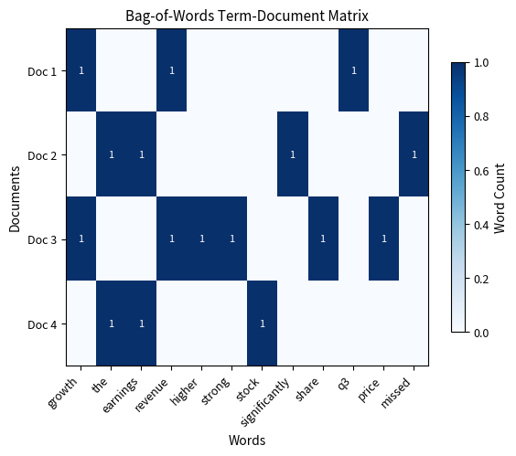
The bag-of-words model is the simplest approach. It treats a document as an unordered collection of words, ignoring grammar and word order entirely. Under this representation, each unique word in the vocabulary becomes a separate feature dimension, and documents are represented as vectors of word counts or frequencies. The resulting vector space has as many dimensions as there are unique words in the corpus, which can easily reach tens of thousands of dimensions for realistic text collections.

Consider two short sentences about a stock:

• "Revenue growth exceeded expectations"
• "Expectations exceeded by revenue growth"

A bag-of-words representation would treat these identically: both contain the same words with the same frequencies. The model captures what topics are discussed but not how they relate. This limitation reveals a fundamental tradeoff. Simpler models like bag-of-words are computationally efficient and interpretable. However, they sacrifice the nuanced meaning that word order conveys. More sophisticated approaches attempt to recover this lost information, but at the cost of greater complexity.

The bag-of-words matrix shows how documents are represented as vectors of word counts. Document 1 and Document 3 both score highly for revenue and growth, while Documents 2 and 4 share earnings vocabulary. However, This representation cannot distinguish between exceeded expectations (positive) and missed estimates (negative) because word order and grammatical relationships are completely ignored. The vocabulary size of 30 unique words determines the dimensionality of the feature space.

Raw word counts suffer from a significant limitation: common words like "the," "and," and "company" dominate the representation despite carrying little discriminative information. These high-frequency words appear in nearly every document, so their presence tells us almost nothing about what makes any particular document unique or meaningful. If we want our numerical representation to capture the distinctive content of each document, we need a weighting scheme that acknowledges that not all words contribute equally to meaning.

The TF-IDF (Term Frequency-Inverse Document Frequency) weighting scheme addresses this limitation through a simple insight. Words that appear frequently in a specific document but rarely across the broader corpus are likely the most informative features. Words that appear everywhere carry little discriminative power regardless of how often they appear in any single document. This intuition leads to a weighting formula that combines two complementary measurements.

The TF-IDF score for a term $t$ in document $d$ within corpus $D$ combines two components to emphasize distinctive terms while downweighting common ones. It measures both how often a term appears in a specific document (term frequency) and how rare that term is across all documents (inverse document frequency):

where:

• $t$: the term (word) being scored
• $d$: the specific document containing the term
• $D$: the entire corpus (collection of all documents)
• $\text{TF}(t, d)$: term frequency, measuring how often term $t$ appears in document $d$ (typically normalized by document length)
• $\text{IDF}(t, D)$: inverse document frequency, downweighting common terms by measuring how rare $t$ is across the corpus
• $\text{TF-IDF}(t, d, D)$: the combined score, higher values indicate terms that are both frequent in the document and rare in the corpus

The multiplication of these two components creates a weighting scheme. Terms that appear frequently in a specific document but rarely across the corpus receive the highest scores, making them the most distinctive features of that document. This multiplicative structure means that both conditions must be satisfied for a term to receive a high weight. A word appearing frequently in one document but also appearing in every other document will have its high term frequency nullified by a low inverse document frequency. Similarly, an extremely rare word that appears only once in a single document receives a limited boost because its term frequency is low despite its high corpus-level rarity.

The inverse document frequency component quantifies how rare or common a term is across the entire corpus. This measurement provides the mechanism for penalizing ubiquitous terms while rewarding distinctive vocabulary. The formula takes a ratio of the total number of documents to the number of documents containing the term, then applies a logarithmic transformation to moderate the scaling behavior.

The inverse document frequency is computed as:

where:

• $t$: the term being evaluated
• $D$: the entire corpus (collection of documents)
• $|D|$: total number of documents in the corpus (cardinality of set $D$)
• $|\{d \in D : t \in d\}|$: number of documents containing term $t$ (size of the subset where $t$ appears)
• $\log$: natural logarithm function, ensuring the penalty grows gradually rather than explosively

The IDF formula penalizes common words through a logarithmic ratio that captures distinctiveness. To understand why this formula works, consider the extreme cases at both ends of the term frequency spectrum. If a term appears in all documents, the ratio $\frac{|D|}{|D|} = 1$ yields $\log(1) = 0$, assigning zero weight because ubiquitous words provide no discriminative power. This makes intuitive sense: if every document contains the word "the," knowing that a particular document contains "the" tells us nothing useful for distinguishing it from other documents. Conversely, if a term appears in only one document, the ratio $\frac{|D|}{1} = |D|$ maximizes $\log(|D|)$, giving high weight to this uniquely identifying term. Such rare terms are precisely the vocabulary that makes a document distinctive.

The logarithm serves an important mathematical purpose beyond simply computing a ratio. Without the logarithmic transformation, the IDF values would grow linearly with corpus size for rare terms, potentially creating extreme weights that dominate the feature representation. The logarithm ensures the penalty grows gradually, not explosively, creating smooth weighting transitions as term frequency increases. This gradient allows IDF to distinguish between moderately common and very common terms without overweighting rare terms. A term appearing in half the documents receives a moderate penalty, while a term appearing in 90% of documents receives a stronger penalty, but the difference remains manageable and interpretable.

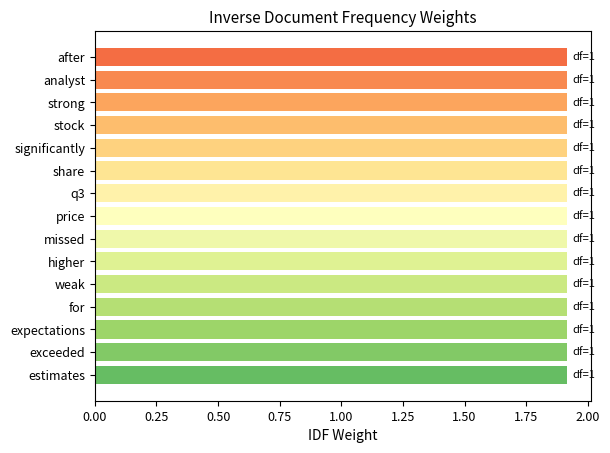
The TF-IDF weighting scheme emphasizes distinctive terms while downweighting common words that appear across multiple documents. Words like missed, downgraded, and exceeded receive higher scores because they appear in only one or two documents: this makes them discriminative features. In contrast, words like the or and (if present) would receive near-zero weights since they appear everywhere. This transformation converts raw word counts into features that better capture what makes each document unique, which is essential for machine learning models to identify meaningful patterns.

Key parameters for TF-IDF vectorization.

• max_features: Maximum number of features to extract. Controls vocabulary size and dimensionality of the feature space.
• ngram_range: Range of n-gram sizes to consider, such as (1,1) for unigrams only or (1,2) for unigrams and bigrams. Higher n-grams capture phrase-level patterns.
• min_df: Minimum document frequency for a term to be included. Filters out rare words that may be noise.
• max_df: Maximum document frequency for a term to be included. Filters out overly common words that provide little discriminative power.

Bag-of-words and TF-IDF treat each word as an independent dimension, ignoring semantic relationships. The word "profit" and "earnings" would be as dissimilar as "profit" and "banana" in these representations, despite their obvious conceptual overlap. This limitation stems from a core assumption. Each word occupies its own orthogonal axis in the feature space with no connection to any other word. In mathematical terms, the dot product between any two different word vectors is zero, treating synonyms and antonyms with equal indifference.

Word embeddings address this limitation by learning dense vector representations where semantically similar words have similar vectors. Rather than assigning each word its own independent dimension, embeddings map words into a shared continuous vector space where geometric proximity reflects semantic relatedness. The key insight, pioneered by Word2Vec and subsequent models, is that a word's meaning can be inferred from the company it keeps. Words appearing in similar contexts should have similar representations. This distributional hypothesis, which states that words with similar distributions have similar meanings, provides the theoretical foundation for learning meaningful representations from raw text alone.

In embedding space, we might find the following.

• "profit" and "earnings" have high cosine similarity
• "bullish" and "optimistic" cluster together
• Vector arithmetic captures relationships such that "CEO" minus "company" plus "country" approximates "president"

Modern transformer-based models like BERT go further, producing contextualized embeddings where a word's representation depends on its surrounding context. The word "bank" receives different embeddings in "river bank" versus "investment bank", resolving ambiguity that plagued earlier approaches.

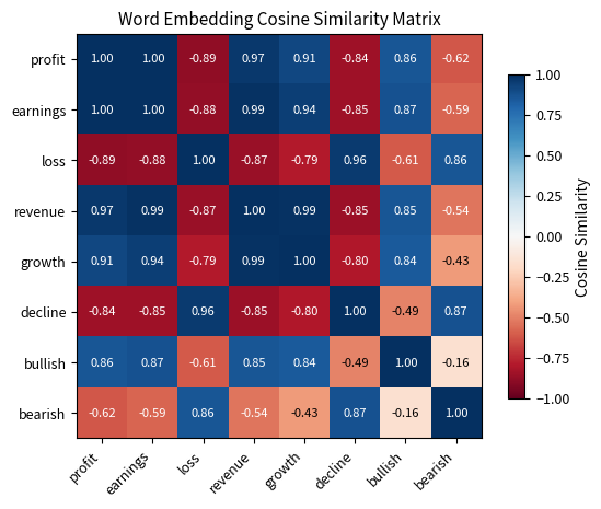
Word embeddings capture semantic similarity through vector geometry. The cosine of the angle between word vectors quantifies how semantically related the words are. This geometric interpretation provides an elegant connection between linguistic meaning and mathematical structure. Words that humans judge as similar tend to point in similar directions in embedding space, while unrelated or opposite words point in different or opposing directions.

The cosine similarity between two word vectors $\mathbf{v}_1$ and $\mathbf{v}_2$ is computed as:

where:

• $\mathbf{v}_1$: embedding vector for the first word
• $\mathbf{v}_2$: embedding vector for the second word
• $\mathbf{v}_1 \cdot \mathbf{v}_2$: dot product of the two vectors, computed as $\sum_i v_{1i} \cdot v_{2i}$, measuring alignment
• $\|\mathbf{v}\|$: Euclidean norm (length) of vector $\mathbf{v}$, computed as $\sqrt{\sum_i v_i^2}$
• $\|\mathbf{v}_1\| \, \|\mathbf{v}_2\|$: product of the two vector lengths, used for normalization
• $i$: index over the dimensions of the embedding vectors
• Cosine similarity ranges from -1 (opposite meanings) to +1 (identical meanings), with 0 indicating orthogonality

This formula measures the cosine of the angle between two vectors, capturing their directional similarity independent of magnitude. The normalization by vector lengths is crucial because it ensures we are measuring directional alignment rather than absolute magnitude. Two vectors could have very different lengths but still point in exactly the same direction, which would indicate semantic similarity. Vectors pointing in the same direction have high positive similarity, opposite directions have negative similarity, and perpendicular vectors have zero similarity. The cosine function provides exactly this behavior: it equals 1 when the angle is zero (parallel vectors), 0 when the angle is 90 degrees (orthogonal vectors), and -1 when the angle is 180 degrees (antiparallel vectors). Semantically similar words have vectors that point in similar directions, yielding high cosine similarity.

The cosine similarity between "profit" and "earnings" of approximately 0.99 indicates these words are used in nearly identical contexts and can be treated as near-synonyms. Conversely, "profit" vs "loss" shows negative similarity, reflecting their opposite meanings. Similarly, "bullish" and "bearish" show strong negative correlation, as expected for antonyms. These geometric relationships allow NLP models to understand that a document discussing "strong earnings growth" is semantically similar to one about "profit increases," even though they share no common words, as the embedding space captures their semantic equivalence.

Key parameters for word embeddings.

• embedding_dim: Dimensionality of the embedding vectors, typically 50 to 300. Higher dimensions capture more nuanced relationships but require more data and computation.
• window_size: Context window for training embeddings. Determines how far apart words can be while still influencing each other's representations.
• min_count: Minimum frequency for a word to receive an embedding. Filters out rare words to reduce vocabulary size.
• pretrained_model: Choice of pretrained embeddings (Word2Vec, GloVe, BERT, FinBERT). Domain-specific models like FinBERT perform better on financial text.

Sentiment analysis (determining whether text expresses positive, negative, or neutral views) is the most common NLP application in quantitative finance. The intuition is straightforward: positive news should correlate with positive price movements, negative news with declines. Implementation, however, requires attention to domain-specific language and the unique characteristics of financial communication.

The simplest sentiment analysis methods use predefined word lists: positive words add to sentiment, negative words subtract. The Loughran-McDonald financial sentiment dictionary, specifically developed for financial text, has become a standard resource.

Generic sentiment dictionaries perform poorly on financial text because many words have domain-specific meanings. In everyday English, liability is negative. In finance, it is a neutral accounting term. Volatile might be negative in most contexts, but in finance it describes a factual characteristic of returns. The Loughran-McDonald dictionary addresses these issues by classifying words based on their financial context.

Converting word counts into a standardized sentiment metric requires capturing net sentiment intensity while controlling for document length. This normalization matters because we need to compare sentiment across documents of varying lengths. Without it, a 1000-word document with 10 positive words appears more positive than a 100-word document with 5 positive words, even though the shorter document has five times the sentiment density. By dividing by total words, we obtain a measure of sentiment intensity that is comparable across documents regardless of their length.

The sentiment score is computed as the difference between positive and negative word counts, normalized by document length. The score ranges from approximately -1 (all words negative) to +1 (all words positive), with 0 indicating neutral or balanced sentiment.

where:

• $N_{\text{positive}}$: count of words in the document that match the positive sentiment dictionary
• $N_{\text{negative}}$: count of words in the document that match the negative sentiment dictionary
• $N_{\text{total}}$: total word count in the document (all words, not just sentiment words)
• The score ranges from approximately -1 (all words negative) to +1 (all words positive), with 0 indicating neutral or balanced sentiment

This provides a standardized measure between -1 (maximally negative) and +1 (maximally positive). The numerator captures the net sentiment (positive minus negative words), while the denominator normalizes by document length. Without normalization, longer documents would mechanically have higher absolute scores even if their sentiment intensity was the same. The theoretical bounds of -1 and +1 are achieved only in extreme cases where every word matches the sentiment dictionaries. In practice, most documents contain many neutral words, so sentiment scores typically fall in a much narrower range around zero.

Dictionary-based approaches are transparent, fast, and require no training data. The results show how word counts translate directly to sentiment scores. Text 1 with 3 positive words and 0 negative words receives a strongly positive score, while Text 2 with multiple negative terms receives a negative score. Text 3, which uses balanced or neutral language, scores near zero.

However, these approaches have limitations. They cannot handle negation: not good incorrectly receives a positive score because it contains good. They also cannot understand context-dependent meanings and fail to detect sarcasm. The phrase surprising lack of losses might be positive, but a dictionary approach would count lack and losses as negative.

Key parameters for dictionary-based sentiment analysis.

• lm_positive: Set of words indicating positive sentiment in the financial domain. Domain-specific dictionaries like Loughran-McDonald perform better than general sentiment lexicons because words like "liability" or "volatile" have different connotations in finance.
• lm_negative: Set of words indicating negative sentiment. Must be carefully curated to avoid false positives from neutral financial terminology.
• normalization_method: How to aggregate word counts into scores. Here we use net count divided by total words. Normalization by document length prevents longer documents from mechanically receiving higher absolute scores.

Machine learning approaches learn sentiment patterns from labeled training data, capturing complex relationships that dictionary methods miss. These models recognize that beat estimates is positive even if neither word appears in a sentiment dictionary.

For financial sentiment, training data typically comes from:

• Analyst recommendation changes (upgrade = positive, downgrade = negative)
• Stock returns following news (positive return = positive sentiment)
• Human-labeled samples from specialized providers

Let's implement a complete sentiment classification pipeline using real financial news data:

The model learns to associate certain words and phrases with sentiment categories. Let's examine what features the model considers most predictive:

The learned coefficients quantify each feature's contribution to sentiment prediction. Positive coefficients mean words that increase the probability of that sentiment class. Negative coefficients decrease it. The magnitude reflects predictive strength, with larger absolute The learned coefficients reveal intuitive patterns: words like "beat," "strong," and "growth" have positive coefficients, while "miss," "decline," and "downgrade" have negative coefficients. The model captures both individual words and bigrams (word pairs), enabling it to distinguish "earnings beat" from "earnings miss" despite both containing "earnings." Phrase-level features like "layoffs" and "record quarterly" carry additional sentiment that individual words alone cannot capture. Parameters

Key parameters for machine learning sentiment classification.

• max_features: Maximum number of TF-IDF features to extract here 100. Higher values capture more vocabulary but increase dimensionality and risk of overfitting.
• ngram_range: Range of n-gram sizes to consider, here 1 to 2 meaning individual words and word pairs. Including bigrams helps capture phrases like "beat estimates" that have different meaning than constituent words.
• test_size: Proportion of data held out for testing, here 0.3 or 30%. Essential for evaluating generalization performance.
• max_iter: Maximum iterations for logistic regression solver (here 1000). Must be sufficient for convergence.
• random_state: Random seed for reproducibility of train/test splits and model initialization.

Modern NLP has been transformed by deep learning, particularly transformer architectures. Pre-trained models like FinBERT, a BERT variant fine-tuned on financial text, achieve state-of-the-art performance on financial sentiment tasks by understanding context, handling negation, and generalizing across varied expressions of similar concepts.

The context-aware model demonstrates superior handling of linguistic nuance compared to dictionary methods. For Earnings did not meet expectations, the model correctly identifies negative sentiment by understanding that not meet negates the neutral phrase meet expectations. For Despite challenges, revenue remained strong, the model recognizes the contrastive structure and correctly emphasizes the positive outcome rather than the negative setup. These examples show how transformer-based architectures capture semantic relationships that simpler bag-of-words approaches miss.

Deep learning models excel at handling linguistic complexity, including negation, sarcasm, hedging language, and implicit sentiment. The phrase did not meet expectations is correctly classified as negative despite containing neither obvious negative words nor being a simple negation of a positive phrase. This contextual understanding represents a substantial advance over dictionary methods.

Key parameters for deep learning sentiment models.

• pretrained_model: Choice of transformer architecture such as BERT, FinBERT, or RoBERTa. FinBERT is specifically fine-tuned on financial text and typically performs best for financial sentiment.
• max_length: Maximum sequence length for tokenization, typically 128 to 512 tokens. Longer sequences capture more context but increase computational cost.
• learning_rate: Controls how quickly the model adapts during fine-tuning. Financial text typically requires lower learning rates than general text.
• num_epochs: Number of training passes through the data. More epochs improve fit but risk overfitting.

Let's build a complete pipeline that converts financial news into a tradable sentiment signal. This example demonstrates the practical workflow from raw text to portfolio positioning.

The sample shows the structure of our simulated news feed with dates, tickers, headlines, and true sentiment labels. The distribution across positive, negative, and neutral sentiment is roughly balanced, providing a realistic test dataset. We'll now process all news through our sentiment model and aggregate to daily stock-level signals.

The summary statistics reveal how sentiment signals vary across stocks. The mean values hovering near zero reflect our dollar-neutral construction, where positive and negative signals balance out over time. Standard deviations around 0.1-0.2 indicate moderate volatility in sentiment, with extremes ranging from approximately -0.4 to +0.4. These bounded ranges prevent any single stock from dominating portfolio positions.

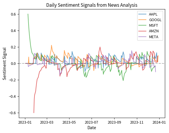
The time series visualization reveals how sentiment signals evolve across different stocks throughout the year. The signals oscillate around zero, reflecting the balance between positive and negative news flow. This pattern is expected from our construction where sentiment scores are normalized to have approximately zero mean. Periods where a stock's line rises above zero indicate accumulating positive sentiment, while dips below zero signal negative news predominance. The crossing patterns show how relative sentiment rankings change: stocks that outperformed sentiment-wise earlier may underperform later. The exponential decay smoothing prevents signals from reacting too sharply to individual news items while still capturing sustained sentiment trends. These dynamic patterns form the basis for constructing market-neutral long-short portfolios.

The sentiment signal exhibits the classic characteristics of alpha factors: mean-reverting oscillations around zero with occasional persistent trends. The exponential weighting ensures recent news has more impact while allowing sentiment to decay over time if no new information arrives.

Following our discussion of factor investing from Chapter 4, we can convert sentiment signals into portfolio weights. The challenge arises because raw sentiment signals have different scales across assets and time periods, making direct comparison difficult. A sentiment score of 0.3 for one stock might represent a strong signal, while the same value for another stock with more volatile sentiment might be unremarkable. You need to standardize signals to a common scale to compare their strength fairly across assets.

Z-score normalization addresses this by standardizing signals to have zero mean and unit variance within each cross-section. The transformation expresses each signal as the number of standard deviations from the cross-sectional average, creating a uniform scale for meaningful comparison across assets. This approach is essential for portfolios where we allocate capital based on relative signal strength rather than absolute signal values.

The z-score transformation centers signals around the cross-sectional mean and scales them by standard deviation:

where:

• $i$: index identifying a specific asset in the portfolio universe
• $s_i$: raw sentiment signal for asset $i$ (from our earlier computations)
• $\bar{s}$: mean sentiment across all assets, computed as $\bar{s} = \frac{1}{N}\sum_{j=1}^{N} s_j$ where $N$ is the number of assets
• $\sigma_s$: standard deviation of sentiment signals across assets, computed as $\sigma_s = \sqrt{\frac{1}{N}\sum_{j=1}^{N}(s_j - \bar{s})^2}$, measuring dispersion
• $z_i$: standardized z-score for asset $i$, representing how many standard deviations $s_i$ is from the mean

This transformation centers signals around zero (subtracting the mean) and scales them to a common standard deviation (dividing by $\sigma_s$). The centering step ensures that the average z-score across all assets is exactly zero, which is a prerequisite for constructing dollar-neutral portfolios. The scaling step normalizes the dispersion so that a z-score of +1 always means "one standard deviation above average" regardless of the underlying signal's natural scale. Assets with above-average sentiment receive positive z-scores, while those with below-average sentiment receive negative z-scores. The magnitude indicates how many standard deviations the signal is from average, providing an intuitive measure of signal strength.

After computing z-scores, you convert them into portfolio weights. Unconstrained z-scores could lead to extreme leverage if used directly. A stock with a z-score of 3 would receive three times the allocation of a stock with a z-score of 1, and the total gross exposure would depend on the particular z-score distribution on each day. We solve this by normalizing so that the total gross exposure (sum of absolute weights) equals 1 (or 100%), creating a controlled leverage profile.

The portfolio weight for each asset is computed as:

where:

• $i$: index for the asset being weighted
• $j$: index running over all assets in the portfolio universe
• $z_i$: standardized z-score for asset $i$ (from the previous formula)
• $w_i$: portfolio weight for asset $i$ (can be positive for long or negative for short positions)
• $|z_j|$: absolute value of z-score for asset $j$
• $\sum_j |z_j|$: sum of absolute z-scores across all assets, normalizing total gross exposure to 1

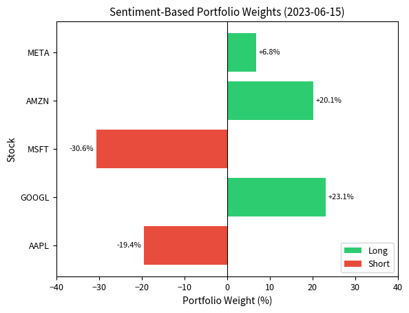
This normalization constrains gross exposure (sum of absolute weights) to exactly 1, preventing excessive leverage while preserving the relative ranking of signals. The denominator sums absolute values rather than raw values because we want to account for both long and short positions when computing total exposure. Assets with positive z-scores receive long positions proportional to their signal strength, while negative z-scores generate short positions. The absolute value denominator ensures both long and short legs contribute to the exposure constraint, creating a balanced long-short portfolio. Because the z-scores were already centered around zero, the sum of positive z-scores approximately equals the sum of absolute negative z-scores, resulting in a portfolio that is naturally dollar-neutral.

The resulting portfolio is dollar-neutral: with net exposure of 0.0000 (effectively zero), it positions stocks according to relative sentiment. The gross exposure of 1.0000 indicates we are fully invested long and short in equal notional amounts. Stocks with the most positive sentiment receive long weights, while those with negative sentiment get short weights. This follows the long-short factor portfolio construction we covered in Part IV.

Key parameters for sentiment-based portfolio construction.

• method: Weighting scheme, here 'zscore' or 'rank'. Z-score weighting normalizes signals by their cross-sectional mean and standard deviation, while rank-based weighting uses ordinal rankings.
• halflife: Decay rate for exponential weighting of historical sentiment, here 5 days. Controls how quickly old sentiment signals lose influence.
• alpha: Smoothing parameter for exponential weighted moving average, computed as $1 - \exp(-\ln(2)/\text{halflife})$. Lower alpha means slower response to new information.
• clip_threshold: Maximum absolute z-score allowed, here 3. Winsorizes extreme values to prevent outliers from dominating portfolio weights.

One of the most celebrated alternative data applications uses satellite imagery to count cars in retail parking lots. The logic is simple: more cars mean more shoppers and stronger sales.

RS Metrics and Orbital Insight pioneered commercial applications of this data, processing satellite images of thousands of retail locations daily. The data provided investors with near-real-time sales indicators, as data became available weeks before quarterly earnings reports.

Studies documented significant predictive power. Analysis of parking lot data for Walmart stores showed correlation with same-store sales growth, with the satellite data available 4 to 6 weeks before official announcements. Early adopters generated substantial alpha by positioning before earnings surprises were publicly known.

However, this edge has diminished as the data became widely available. By 2020, multiple vendors offered similar products, and the information advantage had largely been arbitraged away. The case illustrates both the potential of alternative data and its inevitable decay as adoption spreads.

The relationship between social media sentiment and asset prices has been extensively studied, with mixed results. Early research by Bollen et al. (2011) found that Twitter mood indicators could predict stock market movements with claimed accuracy around 87%. These results generated enormous interest in social media as an alpha source.

Subsequent research tempered enthusiasm. Many findings didn't replicate out of sample, and simple sentiment measures proved unreliable. However, more sophisticated approaches continue to show promise:

• Event detection: Social media can identify breaking news before it appears in traditional sources, providing a speed advantage measured in minutes.
• Volume spikes: Unusual social media activity around a stock often precedes volatility, which is useful for options strategies.
• Consumer sentiment: Aggregate social sentiment about products or brands can provide leading indicators for company performance.

The GameStop episode of January 2021 demonstrated social media's market-moving potential, as coordinated retail trading driven by Reddit discussions created one of the largest short squeezes in market history. While this event was exceptional, it showed that social media sentiment can drive markets, not just reflect them.

Quarterly earnings calls contain rich information beyond the reported numbers. Managers' word choices, speaking patterns, and responses to analyst questions reveal confidence, deception, or uncertainty that financial numbers cannot.

Research has documented several predictive linguistic patterns.

• Complexity and obfuscation: Companies using more complex language in calls tend to underperform, possibly because managers use complexity to obscure poor results.
• Certainty language: Management's use of words conveying certainty (definitely, absolutely) versus hedging (possibly, might) correlates with future performance.
• Emotional tone: Negative emotional language in calls predicts negative returns even when controlling for actual financial results.
• Question evasion: When executives fail to directly answer analyst questions, it often precedes negative surprises.

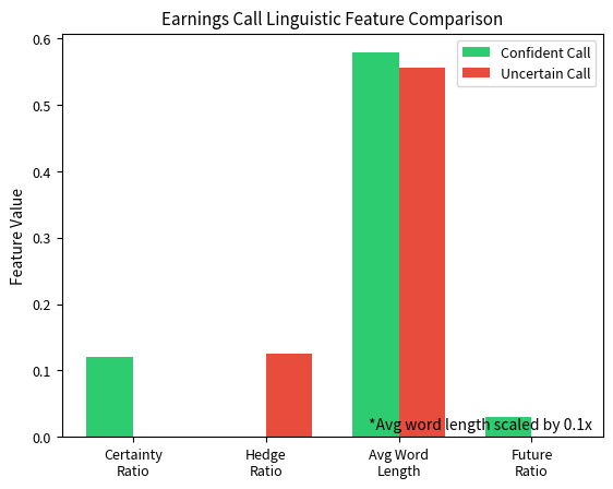
The contrast between the two snippets is striking. The confident call shows high certainty language (certainty ratio of 0.0667) and low hedging (hedge ratio of 0.0000), while the uncertain call exhibits the opposite pattern with lower certainty (0.0000) and higher hedging (0.0800). When aggregated across thousands of calls, these linguistic signatures provide statistically meaningful predictive signals.

Key parameters for earnings call text analysis:

• certainty_words: Set of words indicating high certainty such as 'definitely', 'certainly', or 'absolutely'. Higher certainty language often correlates with management confidence.
• hedge_words: Set of words indicating hedging or uncertainty, such as 'possibly', 'maybe', or 'might'. Excessive hedging may signal underlying concerns.
• future_words: Set of forward-looking terms, such as 'will', 'expect', or 'anticipate'. Tracks management's orientation toward future prospects.
• avg_word_length: Proxy for linguistic complexity. Longer words may indicate obfuscation or technical language.

Alternative data and NLP present unique challenges that distinguish them from traditional quantitative approaches. Understanding these limitations helps you form realistic expectations and build robust systems.

When satellite parking lot data was available to only a few funds in 2015, it generated significant alpha. By 2020, with dozens of subscribers to similar services, the informational advantage had largely disappeared. Prices adjusted more quickly to the signal, leaving fewer opportunities for profitable trading.

This decay creates a perpetual search for new data sources. Academic factors may persist for decades. Alternative data advantages typically last months to years. Maintaining an edge requires continuous innovation in data sourcing and processing, not just better modeling of data you already have. The most successful alternative data firms build data moats through exclusive relationships with data providers, proprietary collection infrastructure, or analytical capabilities that competitors struggle to replicate.

Alternative datasets are typically far noisier than traditional financial data. Social media sentiment is contaminated by bots, sarcasm, and non-financial content. Satellite imagery is affected by weather and parking lot layout changes. Web scraping captures spam and irrelevant content.

This noise makes overfitting a serious risk. Machine learning models with high-dimensional text features and noisy targets can memorize spurious patterns that don't generalize. Rigorous out-of-sample validation and cross-validation are essential safeguards, though even these may not reveal biases specific to particular time periods or market conditions.

Selection biases also pervade alternative data. Social media users are not representative of the general population, credit card data captures only electronic transactions, and satellite coverage may be better for some geographies than others. These biases can create systematic prediction errors that only become apparent when market conditions change.

Alternative data requires extensive preprocessing before it can feed into models. Text must be cleaned of formatting artifacts. Entities must be identified and disambiguated. For example, does "Apple" refer to the company or the fruit? Sentiment must be extracted in context. Each preprocessing step introduces potential errors and assumptions.

Data quality issues pervade alternative datasets. News feeds contain duplicates, incomplete articles, and misattributed sources. Social media includes spam, bot content, and foreign-language posts. Web-scraped data often has parsing errors and site format changes. Geospatial data requires georeferencing, cloud removal, and temporal alignment.

Data engineering typically consumes a larger portion of alternative data projects than modeling does. The principle 'garbage in, garbage out' applies especially strongly when raw inputs are messy and unstructured.

Historical alternative data often differs from what was actually available in real-time. News articles may be timestamped to publication time but weren't accessible until minutes or hours later. Social media APIs may return different results depending on when they're queried. Satellite images might be revised after initial release.

It's hard to build backtests that accurately reflect what data was available historically. Point-in-time data (snapshots of what was actually known) is ideal but often impossible for alternative datasets that weren't collected until recently. This lookback bias inflates historical performance estimates.

The use of alternative data raises important ethical and legal questions that quantitative practitioners must carefully navigate. Regulations including GDPR, CCPA, and securities laws constrain data collection, usage, and trading.

Much alternative data comes from individual behavior (credit card transactions, mobile phone locations, social media posts, and web browsing patterns). Even when anonymized and aggregated, this data can raise privacy concerns.

Compliance considerations:

• Consent and purpose limitation: Ensure data was collected with appropriate consent for investment use. Data collected for one purpose typically cannot be used for another.
• Anonymization adequacy: Verify that aggregated data is truly anonymous. Sparse high-dimensional data like credit card transactions can often be de-anonymized.
• Geographic variation: Privacy regulations differ by jurisdiction. GDPR strictly regulates EU personal data. CCPA grants California residents specific privacy rights.

Reputable vendors provide compliance documentation and legal opinions, but you remain ultimately responsible. You must conduct due diligence on data sourcing and review contracts with legal counsel.

Securities laws prohibit trading on material non-public information (MNPI). Alternative data creates gray areas. For example, when does aggregated private sector data become public? If a fund pays for exclusive access to transaction data, does that constitute MNPI?

Legal consensus generally accepts properly sourced alternative data if it doesn't come from breaches of fiduciary duty or contractual obligations. Data scraped from public websites is generally considered public information. Aggregated and anonymized transaction data, properly licensed, is typically permissible.

However, several edge cases remain legally uncertain:

• Corporate insiders who sell data about their own company
• Employees who leak internal metrics
• Hacked or stolen data that becomes available
• Data obtained through deceptive collection practices

Manage these risks with conservative compliance policies, clear documentation of data sources, and legal review of novel datasets.

The concentration of alternative data advantages among well-resourced funds raises questions of market fairness. If only a few large quantitative funds can afford satellite imagery, credit card data feeds, and NLP infrastructure, does this create an uneven playing field that harms market integrity?

Regulators have generally not acted against alternative data usage; however, increased scrutiny seems likely. The European Union's MiFID II requires evidence that algorithmic trading strategies don't disrupt markets. Future regulations may require transparency about alternative data usage.

The GameStop episode also highlighted how social media analysis can intersect with market manipulation concerns. Monitoring social media for coordinated pump-and-dump schemes has become a compliance priority, and funds using social sentiment must distinguish between legitimate information aggregation and trading on manipulated signals.

Deploying alternative data strategies requires infrastructure and processes beyond model development.

Alternative data arrives continuously from diverse sources with varying formats, latencies, and reliability. A robust pipeline must handle:

• Ingestion: APIs, FTP drops, web scraping, and email parsing
• Validation: quality checks, completeness verification, and anomaly detection
• Transformation: parsing, cleaning, entity resolution, and feature extraction
• Storage: time-series databases, document stores, and data lakes
• Serving: low-latency access for real-time signals and historical access for backtesting

The engineering investment required often exceeds the modeling effort. Many projects fail not because signals don't exist, but because pipelines cannot reliably deliver clean features to production.

Most practitioners buy alternative data rather than collect it. Evaluate vendors on these factors:

• Coverage and history: Which markets the data covers and how far back history extends.
• Timeliness: How quickly the data is available after real-world events.
• Quality and consistency: Whether the data has gaps, revisions, or methodology changes.
• Exclusivity: How many other clients subscribe and how quickly you expect alpha decay.
• Compliance: Clear data provenance and proper licensing.
• Support: Adequate documentation and responsive vendor Trial periods let you evaluate before committing. Start with a narrow use case and expand based on demonstrated value rather than licensing comprehensive data packages upfront. Combining Alternative and Traditional Data

Alternative data rarely replaces traditional fundamental or price data. Rather, it complements them. The most effective approaches combine signals in several ways:

• Ensemble models: Weight alternative data signals alongside traditional factors.
• Conditional models: Use alternative data to time entry or adjust conviction on fundamental theses.
• Validation: Use alternative data to confirm or refute theses from other analyses.

The marginal value of alternative data depends on your existing model. A sentiment signal adds more value to a price-only strategy than to a model that already incorporates fundamental factors.

Alternative data and NLP have significantly expanded the quantitative finance toolkit. By processing information sources traditional analysis ignores (satellite imagery, social media, transaction records, and textual documents), quantitative strategies capture signals that prices and fundamentals cannot.

This chapter covered several key areas:

Alternative data taxonomy encompasses transactional data, geospatial sensors, web and social content, text documents, and specialist industry datasets. The value of alternative data derives from timeliness, granularity, and differentiation from traditional sources. These advantages decay as adoption spreads.

NLP fundamentals transform unstructured text into quantitative features. Bag-of-words and TF-IDF offer simple but limited representations. Word embeddings capture semantic relationships. Transformer models like FinBERT achieve state-of-the-art understanding of context and nuance.

Sentiment analysis is the dominant NLP application in finance. Dictionary methods offer transparency and speed. Machine learning approaches capture complex patterns. Deep learning models handle negation, hedging, and context that simpler methods cannot.

Practical implementation requires robust data pipelines, careful vendor evaluation, and integration with existing strategies. Engineering and data quality challenges typically demand more effort than modeling does.

Challenges and limitations are substantial. Signal decay erodes alternative data advantages over time. Noise, biases, and overfitting risks increase with high-dimensional unstructured inputs. Lookback bias complicates backtesting.

Ethical and legal considerations around privacy, material non-public information (MNPI), and market fairness require careful navigation. Compliance infrastructure and legal review are essential components of any alternative data program.

The next chapter examines cryptocurrency markets, another domain where alternative data (blockchain analysis, exchange order flows, and social media sentiment) plays a central role in quantitative trading.

Ready to test your understanding? Take this quick quiz to reinforce what you've learned about alternative data and natural language processing in quantitative finance.