

Explore cryptocurrency market microstructure, adjust quantitative strategies for extreme volatility, and manage unique risks in 24/7 decentralized trading.
Choose your expertise level to adjust how many terms are explained. Beginners see more tooltips, experts see fewer to maintain reading flow. Hover over underlined terms for instant definitions.
Cryptocurrency Markets and Quant Trading
Cryptocurrency markets represent the most significant structural innovation in financial markets since electronic trading transformed equities in the 1990s. Unlike traditional asset classes we have studied throughout this textbook, cryptocurrencies operate on decentralized blockchain networks, trade continuously across hundreds of global exchanges, and exhibit volatility that dwarfs anything seen in conventional markets. For you, this combination creates both exceptional opportunities and unique challenges.
The emergence of Bitcoin in 2009 introduced a new paradigm: programmable, borderless money secured by cryptographic proofs rather than institutional trust. Ethereum followed in 2015, enabling smart contracts that execute automatically when predefined conditions are met. Today, the cryptocurrency market encompasses thousands of digital assets with a combined market capitalization that has at times exceeded $3 trillion, attracting institutional capital and sophisticated quantitative strategies.
This chapter examines cryptocurrency markets through the lens of quantitative finance. We will explore the market microstructure that makes crypto trading fundamentally different from traditional assets, adapt the statistical arbitrage, momentum, and market-making strategies from earlier chapters to this new domain, and carefully analyze the risks that have bankrupted many crypto-focused funds. The techniques from our discussions of mean reversion, trend following, and high-frequency trading all apply here, but require significant modifications to account for the unique characteristics of crypto markets.
Cryptocurrency Fundamentals
Before diving into trading strategies, we need to understand what cryptocurrencies actually are and how they differ from traditional financial instruments.
What is a Cryptocurrency?
A cryptocurrency is a digital asset that uses cryptographic techniques to secure transactions and control the creation of new units. Unlike fiat currencies issued by central banks, cryptocurrencies operate on decentralized networks where no single entity has control. The innovation that made this possible was the blockchain: a distributed ledger that records all transactions in chronologically ordered blocks, each cryptographically linked to its predecessor.
To appreciate why this innovation matters for financial markets, consider the fundamental problem that cryptocurrencies solve. In traditional finance, trusted intermediaries such as banks and clearinghouses verify transactions and maintain authoritative records. This centralization creates single points of failure and requires participants to trust these institutions. The blockchain replaces this trust-based model with a mathematical one, where the integrity of the transaction history is guaranteed by cryptographic proofs that any participant can independently verify. This shift from institutional trust to cryptographic verification has profound implications for market structure, as we will see throughout this chapter.
A blockchain is a distributed database that maintains a continuously growing list of records (blocks) secured against tampering and revision. Each block contains a cryptographic hash of the previous block, a timestamp, and transaction data. This structure makes it computationally impractical to modify historical records without detection.
The cryptographic hash function serves as the critical linking mechanism between blocks. When a new block is created, it includes a hash of the entire previous block, creating an unbreakable chain. If anyone attempts to modify a historical transaction, the hash of that block would change, which would invalidate the hash stored in the next block, and so on through the entire chain. This cascading effect means that altering any historical record would require recomputing the hash for every subsequent block, a task that becomes computationally infeasible as the chain grows. For you, this immutability means that blockchain transaction data provides a reliable, tamper-proof record of market activity that can be used for backtesting and signal generation.
The key properties that make cryptocurrencies interesting for you include:
- Digital scarcity: Bitcoin, for example, has a hard cap of 21 million coins that will ever exist. This predetermined supply schedule contrasts sharply with fiat currencies where central banks can expand the money supply.
- Permissionless access: Anyone with an internet connection can participate in crypto markets without requiring approval from banks or brokers.
- Pseudonymous transactions: While all transactions are publicly recorded, participants are identified by cryptographic addresses rather than names.
- Settlement finality: Transactions, once confirmed on the blockchain, cannot be reversed or disputed like credit card chargebacks.
Major Cryptocurrencies
The cryptocurrency market has a clear hierarchy based on market capitalization and trading volume:
- Bitcoin (BTC) remains the dominant cryptocurrency, typically representing 40-60% of total crypto market capitalization. It serves primarily as a store of value and speculative asset, with limited programmability beyond simple transfers.
- Ethereum (ETH) is the second-largest cryptocurrency and the foundation for most decentralized finance (DeFi) applications. Ethereum's smart contract functionality enables complex financial instruments to be built directly on the blockchain.
- Stablecoins like Tether (USDT) and USD Coin (USDC) are cryptocurrencies designed to maintain a stable value, typically pegged to the US dollar. They serve as the primary medium of exchange in crypto markets, similar to how cash serves in traditional finance. For you, stablecoins are essential because they allow you to move in and out of positions without converting to fiat currency.
- Altcoins is the catch-all term for the thousands of other cryptocurrencies. These range from serious projects with novel technological approaches to meme coins with no fundamental value proposition.
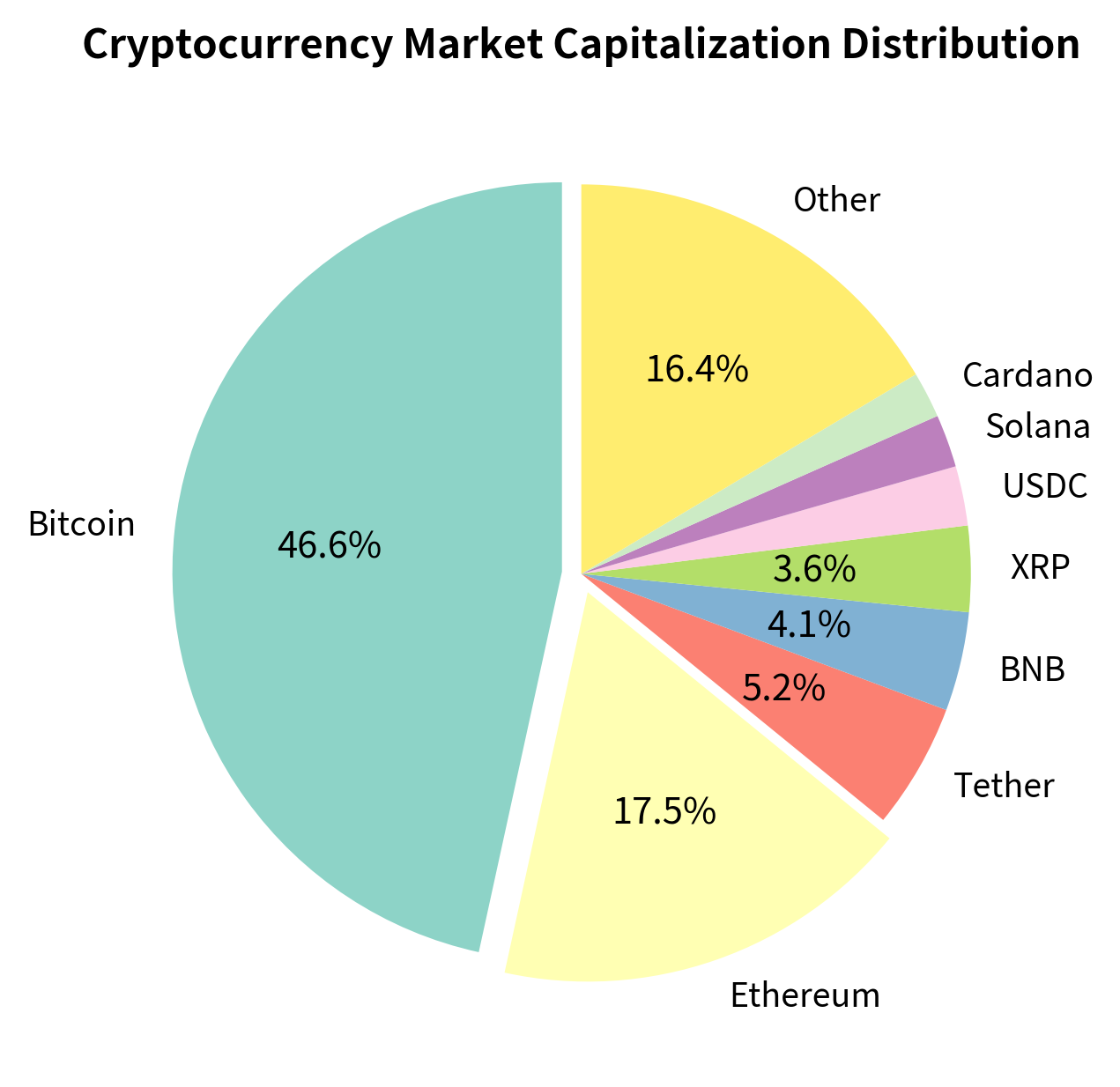
The concentration of market capitalization in Bitcoin and Ethereum has important implications for quantitative strategies. These two assets have the deepest liquidity and most developed derivatives markets, making them the primary focus for institutional traders.
Market Structure
Cryptocurrency market structure differs fundamentally from the traditional exchange models we discussed in earlier chapters. Understanding these differences is essential for developing effective trading strategies.
Centralized Exchanges (CEX)
Centralized exchanges function similarly to traditional exchanges, maintaining order books and matching buyers with sellers. However, there are critical differences:
- Custodial model: When you deposit assets on a centralized exchange, you transfer ownership of those assets to the exchange. The exchange maintains an internal ledger of your balance, and you must trust them to honor withdrawals. This creates counterparty risk that simply does not exist when trading equities through a regulated broker.
- Global fragmentation: Unlike equities, where a single exchange typically dominates trading in each stock, cryptocurrency trading is fragmented across hundreds of exchanges worldwide. This fragmentation creates arbitrage opportunities but also complicates execution.
- Variable fee structures: Exchange fees typically follow a maker-taker model, with fees ranging from 0.01% to 0.5% depending on the exchange and trading volume. This is significantly higher than equity markets, where institutional traders might pay fractions of a basis point.
Major centralized exchanges include Binance (the largest by volume), Coinbase (the most prominent US-regulated exchange), and Kraken. Each exchange has different trading pairs, fee structures, and liquidity profiles.
Decentralized Exchanges (DEX)
Decentralized exchanges represent a fundamentally different approach to trading. Instead of a central order book, most DEXs use automated market makers (AMMs) that provide liquidity through smart contracts.
The concept of an automated market maker emerges from a simple but powerful question: what if we could replace human market makers with mathematical formulas? In traditional markets, market makers are sophisticated firms that continuously quote bid and ask prices, managing their inventory and adjusting quotes based on market conditions. An AMM encodes this behavior into an immutable smart contract, removing the need for human intermediaries entirely. The mathematical formula determines prices automatically based on the current state of the liquidity pool, and anyone can trade against this formula at any time.
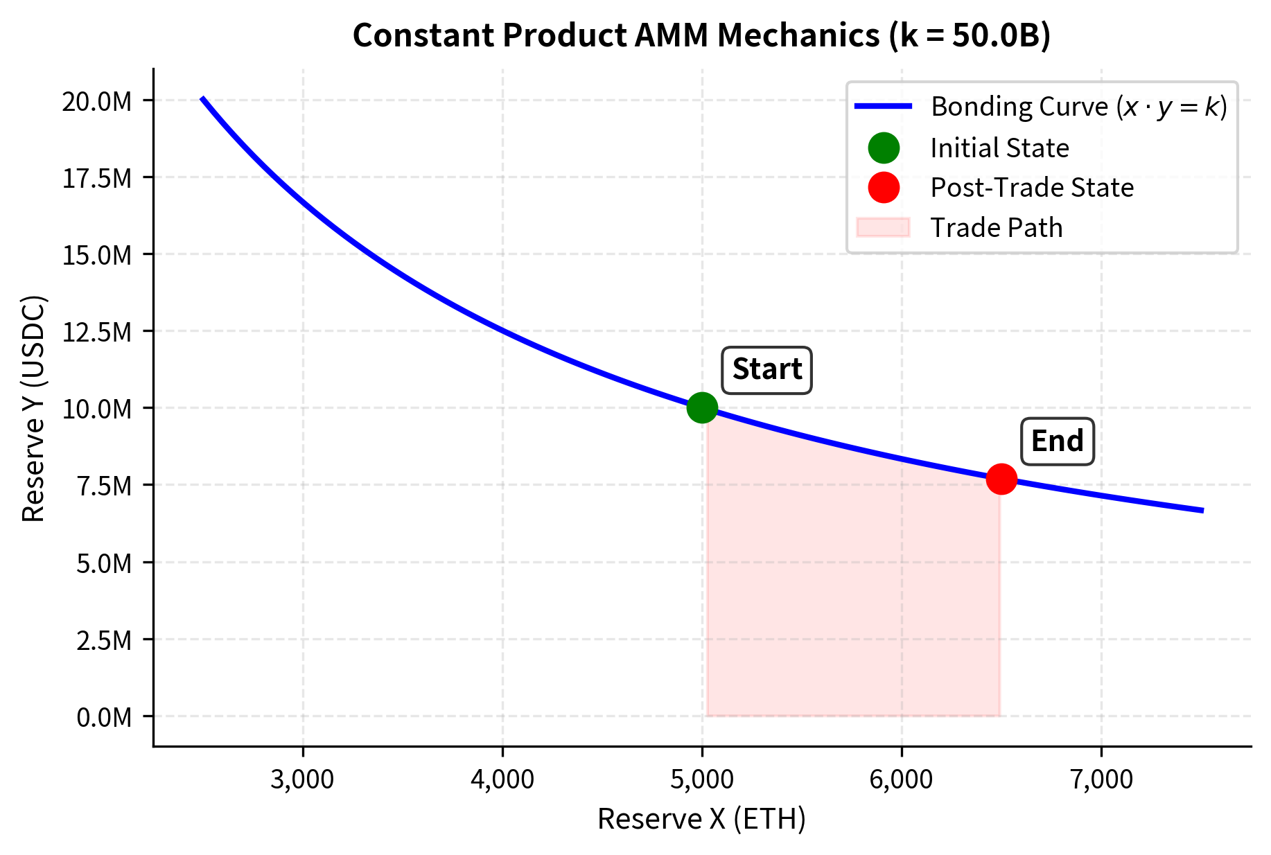
An automated market maker is a smart contract that holds reserves of two or more tokens and allows traders to swap between them at prices determined by a mathematical formula. The most common is the constant product formula:
where:
- : quantity of the first token
- : quantity of the second token
- : invariant constant
This ensures that as one token is bought, its price increases automatically.
The elegance of this formula lies in its simplicity and self-correcting nature. The product of the two reserves must remain constant before and after every trade (ignoring fees for the moment). This constraint creates a hyperbolic relationship between the reserves: as one decreases, the other must increase to maintain the constant. The result is a smooth, continuous pricing curve that never reaches zero for either asset, meaning the pool can always quote a price, albeit at increasingly unfavorable rates for large trades. This constant availability of liquidity, even in extreme market conditions, represents a fundamental departure from order-book markets where liquidity can completely disappear during stress.
The AMM pricing mechanism creates unique dynamics derived from the constant product formula . To understand how prices emerge from this simple equation, let us walk through the mechanics step by step. When you want to swap token X for token Y, you add units of X to the pool. The pool's X reserve increases to , but the constant product constraint demands that remain unchanged. This means the Y reserve must decrease to compensate. Solving algebraically, the new Y reserve must equal , and you receive the difference between the old and new Y reserves.
The price impact measures the percentage deviation of the effective execution price from the spot price . We derive this by first calculating the amount of tokens received (based on the constant product ), then comparing the effective price to the spot price. This derivation reveals why large trades face increasingly unfavorable prices, a phenomenon that will shape our understanding of execution costs in decentralized markets:
where:
- : the trade size (amount of token being sold)
- : the current reserve of the token being sold in the pool
- : the reserve of the other token in the pool
- : the theoretical market price () before the trade
- : the realized average price of the trade
The final expression provides a remarkably intuitive result: the price impact equals your trade size as a fraction of the post-trade reserve. A trade of 10 units into a pool with 100 units would face approximately 9% price impact (10/110), while a trade of 1 unit would face only about 1% impact (1/101). This formula demonstrates that execution price worsens non-linearly as trade size increases relative to liquidity. The relationship is concave, meaning the first units traded suffer relatively little impact, but marginal impact accelerates as the trade size grows. This means large trades face significant price impact, and the market has no concept of a "best bid" or "best offer" in the traditional sense. The following function constant_product_amm implements this pricing logic, calculating the new reserves resulting from a trade and deriving the price impact by comparing the effective execution price to the initial spot price:
The nonlinear price impact on AMMs has profound implications for execution. A 100 ETH sell order in this pool faces approximately 2% price impact, compared to the sub-basis-point impact you might see for equivalent notional in liquid equity markets. This difference arises because AMM liquidity is passive and formulaic, whereas order-book liquidity in traditional markets reflects the active decisions of many sophisticated participants who compete to provide tight spreads. For you, accustomed to equity markets, this magnitude of execution cost requires a fundamental rethinking of strategy capacity and trade sizing.
The mechanics of the constant product formula are best understood visually. The hyperbola defines all possible reserve states. A trade moves the pool's state along this curve. The difference between the slope of the curve at the starting point (spot price) and the slope of the chord connecting the start and end points (effective price) represents the slippage or price impact.
Key Parameters
The key parameters for the Constant Product AMM are:
- x: Reserve of the first token (e.g., ETH). High reserves reduce price impact because the same trade size represents a smaller percentage of the pool.
- y: Reserve of the second token (e.g., USDC). The ratio y/x determines the spot price at which infinitesimally small trades would execute.
- k: The constant product invariant (). This remains fixed during a trade (ignoring fees), serving as the fundamental constraint that generates the pricing curve.
- : The trade size. Larger trade sizes relative to reserves cause exponential price impact because each marginal unit must be purchased at an increasingly unfavorable price along the hyperbolic curve.
24/7 Trading and Global Access
Perhaps the most operationally significant difference for you is that cryptocurrency markets never close. Trading occurs 24 hours a day, 7 days a week, 365 days a year. This creates challenges across multiple dimensions:
- Infrastructure requirements: Systems must run continuously without maintenance windows. Unlike equity trading where you can perform updates over weekends, crypto systems require redundancy and hot-swappable components.
- Staffing and monitoring: Human oversight cannot follow the markets continuously. This places greater emphasis on automated risk controls and alerting systems.
- Volatility timing: Some of the largest price moves occur during what would be "off-hours" in traditional finance, often during weekend periods when liquidity is thinner.
- Funding and margin: Positions must be monitored for margin requirements at all times, not just during market hours.
How Crypto Differs from Traditional Markets
The differences between crypto and traditional markets extend beyond market structure to fundamental characteristics that affect every aspect of quantitative strategy design.
Volatility Regime
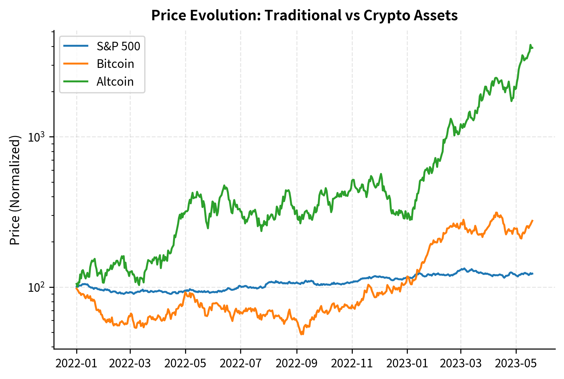
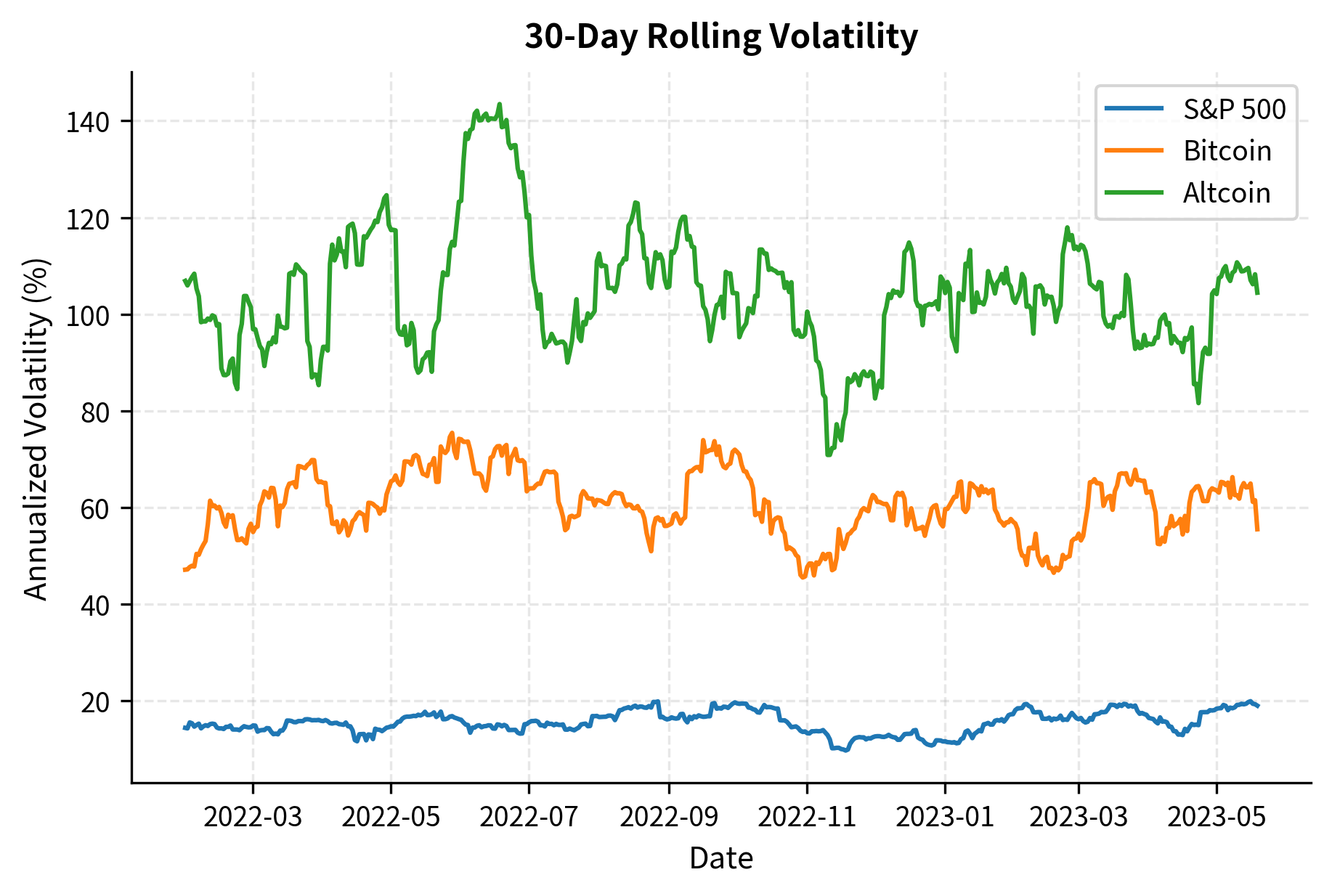
Cryptocurrency volatility operates in a completely different regime compared to traditional assets. While annualized volatility for the S&P 500 typically ranges from 10-25%, Bitcoin regularly exhibits volatility of 50-100%, and smaller altcoins can exceed 200%.
This extreme volatility has several implications for quantitative strategies:
- Position sizing: The position sizing frameworks we discussed in portfolio theory must be adjusted significantly. A 1% allocation to crypto can contribute as much portfolio risk as a 4% allocation to equities.
- Stop losses: Traditional stop-loss levels may be triggered routinely by normal price fluctuations. Stops need to be calibrated to crypto-specific volatility.
- Return expectations: Higher volatility means both higher expected returns for risk-tolerant investors and more severe drawdowns.
Return Distribution Characteristics
Building on our discussion of stylized facts of financial returns from Part III, crypto returns exhibit even more extreme departures from normality:
The higher kurtosis in crypto returns means that extreme events occur more frequently than a normal distribution would predict. This has direct implications for Value-at-Risk calculations, as we discussed in Part V. Historical simulation or fat-tailed distributions like Student's t are essential when modeling crypto risk.
Regulatory Environment
Traditional financial markets operate within well-defined regulatory frameworks with clear rules for trading, disclosure, and investor protection. Cryptocurrency markets exist in a patchwork of regulatory environments:
- United States: The SEC and CFTC have overlapping and sometimes conflicting jurisdictions. Most cryptocurrencies remain in regulatory limbo regarding their classification as securities or commodities.
- Europe: MiCA (Markets in Crypto-Assets) regulation provides a more comprehensive framework, though implementation is ongoing.
- Asia: Approaches vary dramatically, from Japan's licensing regime to China's outright bans.
For you, regulatory uncertainty creates both risks (potential sudden restrictions on trading) and opportunities (regulatory arbitrage and market inefficiencies caused by fragmented oversight).
Market Microstructure Differences
The microstructure of crypto markets differs from traditional markets in ways that directly affect trading strategies:
- No consolidated tape: There is no authoritative source for the "true" price of a cryptocurrency. Each exchange has its own price, and these can diverge significantly during periods of stress.
- Variable tick sizes: Crypto assets can trade to many decimal places, unlike equities with fixed tick sizes. This affects order book dynamics and optimal quote placement.
- Limited short selling: While derivatives markets allow short exposure, directly shorting crypto on spot markets is difficult or impossible on many exchanges.
- Flash crashes and wicks: The combination of thin liquidity at certain price levels and aggressive liquidation mechanisms means crypto markets experience flash crashes more frequently than traditional markets.
Quantitative Strategies in Crypto
The quantitative strategies we have studied throughout Part VI all have applications in cryptocurrency markets, though each requires adaptation to account for the unique characteristics we have discussed.
Statistical Arbitrage Across Exchanges
The fragmentation of crypto markets across hundreds of exchanges creates persistent price discrepancies. As we discussed in our chapter on statistical arbitrage, these discrepancies can be exploited, but the mechanics are more complex in crypto.
The basic cross-exchange arbitrage opportunity occurs when the same asset trades at different prices on different exchanges. At first glance, this seems like free money: buy where the asset is cheap, sell where it is expensive, and pocket the difference. However, several frictions stand between observation and profit. Trading fees consume a portion of the spread, and transferring assets between exchanges takes time and costs money. During that transfer window, prices can move against you. The potential profit must account for all of these factors:
where:
- : net profit from the arbitrage loop
- : price on the exchange where the asset is expensive
- : price on the exchange where the asset is cheap
- : total trading fees (maker and taker) across both venues
- : estimated cost of transferring assets (network fees and time delay risk)
This formula captures the static economics of arbitrage, but the real challenge is dynamic. The prices and are not fixed during execution. Between the moment you identify the opportunity and the moment you complete both legs of the trade, prices will move. If Bitcoin is trading at \$45,000 on Binance and \$45,100 on Coinbase, the \$100 gross spread looks attractive. But if it takes 30 minutes to transfer Bitcoin between exchanges, and Bitcoin's hourly volatility is 1%, there is substantial risk that the price on the expensive exchange will have fallen before you can sell.
We implement this in the CrossExchangeArbitrage class below. The calculate_opportunity method identifies the best buying and selling venues, computes the net profit after all fees, and applies a risk adjustment based on the asset's volatility and the estimated transfer time. The risk adjustment uses a 2-sigma buffer, meaning we subtract two standard deviations of expected price movement from our profit estimate, ensuring we only execute when the opportunity is robust enough to survive adverse price moves:
The challenge with cross-exchange arbitrage is that opportunities are typically small and fleeting. The transfer time between exchanges (which can range from minutes to hours depending on blockchain congestion) introduces significant execution risk. Sophisticated arbitrageurs maintain balances on multiple exchanges to execute immediately, then rebalance during quieter periods. This pre-positioning strategy eliminates transfer risk but requires substantial capital deployment across venues, each of which carries counterparty risk.
Key Parameters
The key parameters for the Cross-Exchange Arbitrage model are:
- Fees: Trading fees (maker and taker) charged by exchanges. High fees increase the spread required for profitability and can turn a seemingly attractive opportunity into a loss.
- Transfer Cost: The cost to move assets between exchanges, including blockchain network fees. During periods of network congestion, these fees can spike dramatically.
- Transfer Time: The duration of the transfer, which exposes you to price risk while assets are in transit. The risk grows with the square root of time, as reflected in the volatility adjustment.
- Volatility: The asset's volatility, used to calculate the risk buffer required to protect against price moves during transfer. Higher volatility demands larger spreads to justify the risk.
Triangular Arbitrage
Within a single exchange, triangular arbitrage exploits pricing inconsistencies across trading pairs. If you can buy BTC with USD, sell BTC for ETH, and sell ETH for USD at prices that net more than your starting USD, a risk-free profit exists. The beauty of triangular arbitrage is that all three trades can execute nearly simultaneously on the same exchange, eliminating the transfer risk that plagues cross-exchange strategies.
To understand why triangular arbitrage opportunities exist, consider that each trading pair on an exchange is essentially an independent market with its own supply and demand dynamics. When a large buyer enters the BTC/USD market, the BTC price rises against USD. But the ETH/BTC market may not adjust immediately, creating a brief window where the implied BTC price through the ETH/BTC pair differs from the direct BTC/USD price.
For three currencies A, B, and C with exchange rates , , and , the arbitrage return is:
where:
- : arbitrage profit (positive values indicate a profitable loop)
- : exchange rate to convert currency A to B
- : exchange rate to convert currency B to C
- : exchange rate to convert currency C back to A
The intuition behind this formula is that if markets are perfectly efficient, converting A to B to C and back to A should return exactly your starting amount, making the product of the three rates equal to 1. Any deviation from 1 represents mispricing that can be exploited. If this expression is positive after accounting for fees, an arbitrage opportunity exists. In practice, each trade incurs a fee that compounds through the loop, so the gross mispricing must exceed three times the single-trade fee rate.
The find_triangular_arbitrage function below evaluates this relationship for a specific triangular path (e.g., USD to BTC to ETH to USD). It calculates the potential return for both directions of the loop, factoring in trading fees at each step. Checking both directions is important because while one direction may show a loss, the reverse direction might be profitable:
In practice, triangular arbitrage opportunities in crypto are captured quickly by automated systems. The opportunities tend to be larger during periods of high volatility when market makers widen spreads asymmetrically across pairs. The key to profitability is execution speed: you who can identify and execute the triangular trade fastest capture the profit before prices adjust. This makes triangular arbitrage a game of latency optimization, similar to high-frequency trading in traditional markets.
Key Parameters
The key parameters for the Triangular Arbitrage model are:
- Rates: Exchange rates for the currency pairs involved in the triangle. Small deviations from the no-arbitrage relationship create opportunities.
- Fee: Trading fee percentage charged on each leg of the trade. Fees compound through the loop, so a 0.1% fee per leg results in approximately 0.3% total cost for the round trip.
- Spread: The difference between the implied cross-rate and the actual cross-rate, which drives the opportunity. This spread must exceed the total fees for the trade to be profitable.
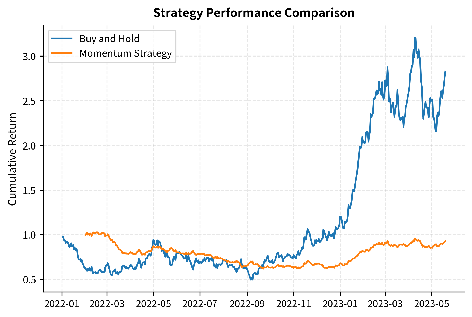
Momentum and Trend Following
As we explored in our chapter on trend following, cryptocurrency markets exhibit strong momentum characteristics. The retail-dominated nature of the market and the influence of social media create trend persistence that can be exploited. Unlike institutional-dominated markets where sophisticated participants quickly arbitrage away mispricings, crypto markets can trend for extended periods as waves of retail traders chase performance.
The psychological dynamics underlying crypto momentum are particularly pronounced. When Bitcoin rises 10% in a week, mainstream media coverage increases, which attracts new retail investors, who buy and push prices higher, generating more media coverage in a self-reinforcing cycle. The same dynamics work in reverse during downtrends, with fear and negative headlines driving selling. These behavioral patterns create momentum that systematic strategies can capture.
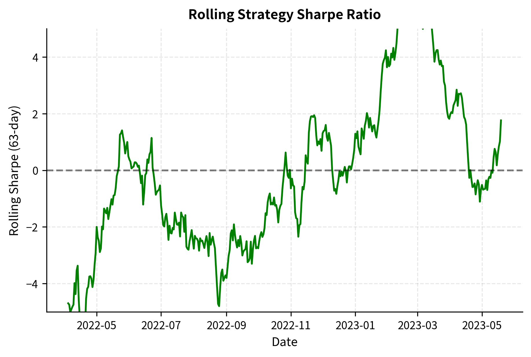
The CryptoMomentumStrategy class implements a volatility-scaled trend following approach. It generates buy/sell signals based on the lookback return sign, scales position sizes inversely to volatility to maintain a constant risk target, and applies a leverage cap to prevent excessive exposure. The volatility scaling is particularly important in crypto because volatility can double or triple within days. Without this adjustment, a fixed position size would expose the strategy to unacceptable risk during high-volatility periods:
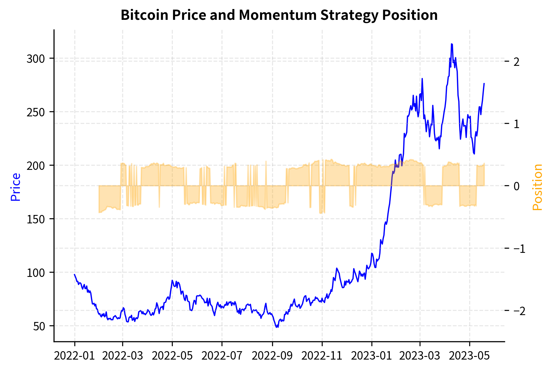
The key adaptations for crypto momentum strategies include:
- Faster lookback periods: Given higher volatility and faster-moving trends, lookback periods of 10-30 days often work better than the 3-12 month horizons common in equity momentum.
- Volatility scaling: Position sizing based on realized volatility is essential to avoid blow-ups during volatile periods.
- Regime awareness: Crypto markets alternate between trending and mean-reverting regimes more dramatically than traditional markets.
Key Parameters
The key parameters for the Crypto Momentum Strategy are:
- Lookback: Period for calculating momentum signal. Shorter windows (10-30 days) often suit crypto's fast cycles because trends develop and exhaust more quickly than in traditional markets.
- Volatility Window: Lookback period for volatility calculation. Used to normalize risk and ensure consistent exposure across varying market conditions.
- Risk Target: Target annualized volatility contribution for the position. A 20% risk target means the position is sized so that, given current volatility, the expected annualized standard deviation of returns is 20%.
- Leverage Cap: Maximum absolute position size allowed to prevent excessive exposure. This hard limit protects against model errors when volatility estimates are stale or unusually low.
Market Making in Crypto
Market making, as we discussed in Part VI, involves continuously quoting bid and ask prices to earn the spread. In crypto markets, the high volatility and relatively thin liquidity create both opportunities and risks for market makers. The opportunity lies in wider spreads: while equity market makers might earn 1-2 basis points per trade, crypto market makers can earn 5-15 basis points or more. The risk is that inventory can quickly accumulate and move against you in a volatile market.
The fundamental market-making model adapts the classic inventory-based approach developed by Avellaneda and Stoikov. The core insight is that you should adjust your quotes based on your current inventory. If you are already long the asset, you want to encourage sales (to reduce your inventory) by quoting a more attractive bid price, and discourage purchases by quoting a less attractive ask price. Conversely, if you are short, you want to encourage purchases and discourage sales.
The optimal bid and ask prices around mid-price depend on inventory :
where:
- : optimal bid and ask quotes
- : current mid-market price
- : base bid-ask spread
- : risk aversion parameter
- : volatility of the asset
- : current inventory position (signed quantity)
The structure of these formulas deserves careful attention. The first two terms on the right side of each equation represent the symmetric spread around mid-price: the bid is half a spread below mid, and the ask is half a spread above. The third term, , is the inventory adjustment that skews both quotes in the same direction. Notice that this adjustment appears with the same sign in both formulas, meaning it shifts the entire quote structure either up or down depending on inventory.
The inventory term causes you to skew quotes to rebalance your position. For example, if you hold a long position (), the inventory adjustment is negative, shifting both bid and ask prices down. Lower prices discourage sellers from hitting the bid (preventing more buying) and encourage buyers to hit the ask (facilitating selling), thus reducing the inventory. The magnitude of this adjustment depends on : higher risk aversion or higher volatility leads to more aggressive inventory management, as the cost of holding a position in a volatile market is higher.
We model this dynamic in the CryptoMarketMaker class. The compute_quotes method calculates optimal bid and ask prices based on the current mid-price, volatility, and inventory level, while simulate_day models the interaction with incoming flow. The simulation assumes a simple model where orders arrive randomly with equal probability of buying or selling, allowing us to observe how inventory evolves and how profits accumulate:
The relationship between inventory management and profitability is crucial. As you absorb flow, your inventory fluctuates, creating risk. The following visualization tracks the inventory and accumulated profit-and-loss (PnL) during the high-volatility simulation. Notice how PnL is volatile due to mark-to-market changes in the inventory value, even as the strategy attempts to capture the spread.
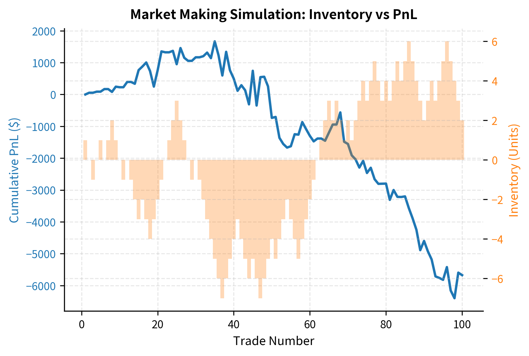
The challenge for you as a market maker is that adverse selection is severe: informed traders or arbitrageurs are more likely to hit your quotes when prices are about to move against you. This means that the flow you receive is not random; it is biased toward trades that will lose money for you. Successful market making requires not just optimal quote placement, but also the ability to detect when incoming flow is likely to be informed and to adjust quotes or withdraw from the market accordingly. This makes quote management and latency critical. We will explore these execution challenges further in Part VII when we discuss market microstructure and execution algorithms.
Key Parameters
The key parameters for the Market Making model are:
- Spread (): The distance between bid and ask quotes. Wider spreads compensate for volatility risk and adverse selection, but reduce the probability of execution.
- : Risk aversion parameter. Higher values lead to more aggressive inventory management, meaning you will skew quotes more strongly to reduce inventory exposure.
- Inventory (): Current net position. Non-zero inventory skews quotes to encourage balancing trades. The further from zero, the more aggressive the skew.
- : Volatility of the asset. High volatility widens the optimal spread to protect against adverse selection and increases the cost of holding inventory, leading to more aggressive inventory management.
Risk Factors Unique to Crypto
Cryptocurrency trading involves risks that simply do not exist in traditional markets. These risks have led to spectacular fund failures and exchange collapses, making risk management even more critical than in traditional quant trading.
Exchange Counterparty Risk
When you hold assets on a centralized exchange, you are exposed to the exchange's solvency and security. The history of crypto is littered with exchange failures:
- Mt. Gox (2014): Once handling 70% of all Bitcoin transactions, collapsed after discovering that 850,000 BTC had been stolen, likely over several years.
- FTX (2022): A top-five exchange by volume that collapsed when it was revealed that customer funds had been commingled with its trading affiliate.
- Numerous smaller exchanges: Have experienced hacks, exit scams, or simply ceased operations.
For you, this means:
- Diversify exchange exposure: Never hold more capital on a single exchange than you can afford to lose.
- Minimize exchange balances: Keep assets in self-custody (hardware wallets) when not actively trading.
- Monitor exchange health: Track exchange reserve proofs, insurance fund levels, and regulatory standing.
Smart Contract Risk
For strategies that interact with decentralized finance protocols, smart contract risk is paramount. Bugs in smart contract code can lead to immediate and irreversible loss of funds.
Notable smart contract failures include:
- The DAO (2016): A reentrancy bug allowed an attacker to drain \$60 million from an early Ethereum investment fund.
- Wormhole (2022): A bridge protocol lost \$320 million when an attacker exploited a signature verification bug.
Mitigating smart contract risk involves:
- Code audits: Only interact with protocols that have been audited by reputable security firms.
- Time in production: Favor protocols that have been operating without incident for extended periods.
- Exposure limits: Treat DeFi allocations as high-risk and size accordingly.
Regulatory Risk
The regulatory landscape for cryptocurrency can shift rapidly. Examples include:
- China banning crypto mining and trading multiple times
- The US SEC classifying certain tokens as securities, affecting their tradability
- Individual exchanges losing access to banking or payment processing
You must maintain flexibility to shift operations across jurisdictions and adapt strategies to changing regulatory requirements.
Liquidity Risk
Crypto markets can experience severe liquidity crises. During market stress, liquidity can evaporate across multiple venues simultaneously as market makers withdraw and arbitrageurs hit capacity limits. Unlike traditional markets where designated market makers have obligations to maintain orderly markets, crypto market makers can and do simply turn off their systems during extreme volatility.
The estimate_liquidity_risk function quantifies this cost. It estimates market impact using a participation-rate model and adds a volatility-based risk charge for the duration of the execution. The participation rate measures what fraction of available liquidity your trade would consume, which directly influences market impact. The model applies a square-root rule for impact, reflecting the empirical observation that impact grows sublinearly with trade size:
These liquidity costs scale non-linearly with trade size, making large positions increasingly expensive to enter and exit. The practical capacity of many crypto strategies is much smaller than equivalent strategies in traditional markets. A strategy that could comfortably manage \$100 million in equities might be constrained to \$10 million or less in crypto markets due to the combination of higher impact costs and wider spreads.
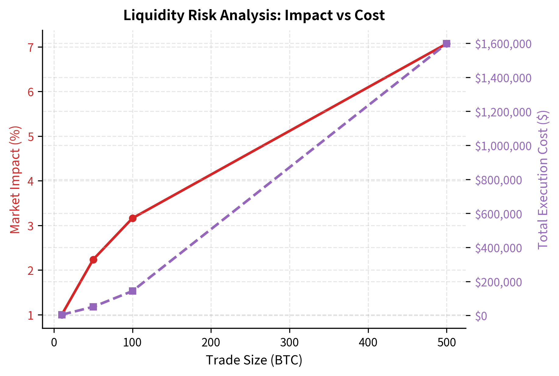
Key Parameters
The key parameters for the Liquidity Risk model are:
- Trade Size: The quantity of the asset to execute. Larger trades incur exponentially higher impact because each marginal unit trades at a worse price.
- Order Book Depth: Cumulative liquidity available at various price levels. Deeper books reduce impact for a given trade size.
- Volatility: Asset volatility used to estimate execution risk. Higher volatility increases the cost of slow execution because prices are more likely to move against you while working the order.
- Participation Rate: The ratio of the trade size to the available depth, determining market impact. This is the primary driver of execution cost.
Crypto in Quantitative Portfolios
As cryptocurrency markets have matured, institutional investors have increasingly considered crypto allocations within broader portfolios. The question is how to integrate an asset class with these unique characteristics.
Correlation Structure
Bitcoin and other cryptocurrencies have exhibited time-varying correlations with traditional assets:
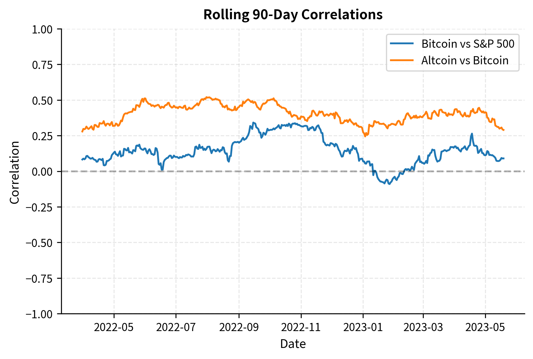
Key observations about crypto correlations:
- Rising equity correlations: During market stress (March 2020, 2022 bear market), Bitcoin has increasingly correlated with equities, reducing its diversification benefit precisely when it would be most valuable.
- High intra-crypto correlations: Most cryptocurrencies are highly correlated with Bitcoin, limiting diversification benefits within the crypto universe.
- Correlation instability: The correlation structure shifts significantly over time, making static allocation models unreliable.
Portfolio Allocation
Given the extreme volatility and unique risks, how should a quantitative portfolio include crypto exposure?
A risk-parity inspired approach allocates capital inversely proportional to volatility to equalize risk contributions. The intuition is straightforward: if Bitcoin is four times as volatile as equities, you should hold one-quarter as much Bitcoin to contribute equal risk to your portfolio. This approach ensures that neither asset dominates the portfolio's risk profile, allowing diversification benefits to accrue.
The target weight calculation (prior to applying maximum limits) is:
where:
- : unconstrained target weight for the crypto allocation
- : current annualized volatility of the cryptocurrency
- : annualized volatility of the equity portfolio
To understand this formula, consider what happens as crypto volatility increases. The term decreases, making the numerator smaller relative to the denominator, which reduces the target weight. Conversely, if crypto volatility decreases toward equity volatility levels, the weights would converge toward 50/50. This inverse weighting mechanism ensures that the asset with higher volatility receives a proportionally lower weight, keeping the risk contribution roughly constant across assets.
In practice, risk-parity allocations to crypto are typically very small. If equity volatility is 16% and crypto volatility is 65%, the risk-parity weight for crypto would be approximately 20% (16/(16+65)). However, most institutional investors apply additional constraints based on operational concerns, liquidity limits, and mandate restrictions.
We then apply the portfolio constraint:
where:
- : final constrained weight
- : maximum allowable position weight (cap)
The calculate_crypto_allocation function implements this framework. It computes the risk-parity weights based on the inverse of annualized volatilities for both crypto and equity components, then applies the maximum weight constraint to determine the final allocation. The function also calculates the resulting portfolio volatility and the risk contribution from the crypto allocation, allowing investors to understand exactly how much of their total risk comes from their crypto position:
The analysis shows that risk-parity principles would suggest very small crypto allocations, typically 1-5% depending on the volatility regime. Even a small capital allocation results in a significant contribution to total portfolio risk. A 10% weight in crypto with 65% volatility contributes far more to portfolio risk than a 90% weight in equities with 16% volatility. This highlights why institutional investors who have added crypto exposure have generally done so in very small amounts, treating it as a satellite position rather than a core holding.
Key Parameters
The key parameters for the Portfolio Allocation model are:
- : Cryptocurrency volatility. The primary driver of allocation size in risk parity, as higher volatility directly reduces the target weight.
- : Equity portfolio volatility. Used as the baseline for risk comparison. The ratio of volatilities determines the relative weights.
- Correlation: The correlation coefficient between crypto and equity. Affects portfolio variance but less critical for simple risk parity weights. However, the instability of this correlation is a key concern for portfolio construction.
- Max Weight: Hard cap on allocation to prevent concentration risk regardless of volatility. This constraint reflects practical considerations such as liquidity limits, operational constraints, and mandate restrictions.
Practical Implementation Considerations
Building quantitative trading systems for cryptocurrency requires addressing several practical challenges beyond strategy design.
Data Infrastructure
Cryptocurrency data is fragmented across exchanges, each with different APIs, rate limits, and data formats. Key considerations include:
- Order book data: Full order book snapshots are essential for market making and execution algorithms but generate enormous data volumes.
- Historical data: Many exchanges do not provide comprehensive historical data, requiring third-party providers or archiving your own.
- On-chain data: Blockchain transaction data provides signals about large holder behavior, exchange flows, and network health.
Execution Infrastructure
The 24/7 nature of crypto markets requires robust, highly available systems:
- Exchange connectivity: Maintain connections to multiple exchanges with automatic failover.
- Order management: Track orders across venues with different latency and confirmation characteristics.
- Risk controls: Implement hard limits on position sizes, loss limits, and circuit breakers that operate continuously.
Reconciliation and Accounting
The combination of multiple exchanges, blockchain transactions, and DeFi interactions creates significant reconciliation challenges:
- Multi-venue positions: Aggregate positions across exchanges, wallets, and protocols.
- Cost basis tracking: For tax purposes, track the cost basis of assets that move between venues.
- Fee accounting: Exchange fees, gas fees, and protocol fees all affect profitability.
Limitations and Impact
Cryptocurrency markets presents unique challenges for you that must be carefully considered alongside the opportunities.
The most fundamental limitation is the relative immaturity and instability of the market infrastructure. Unlike traditional markets where exchanges are regulated utilities with decades of operational history, crypto exchanges are private companies that can fail, be hacked, or change terms arbitrarily. The collapse of FTX in 2022, which was considered one of the most sophisticated and well-regulated exchanges, demonstrated that even sophisticated market participants can misjudge counterparty risk. This forces you to implement operational safeguards that would be unnecessary in traditional markets, adding complexity and cost to trading operations.
The extreme volatility of crypto markets creates both opportunity and danger. While high volatility can generate attractive returns for momentum and volatility strategies, it also means that losses can accumulate rapidly. A strategy that performs well during normal conditions may experience catastrophic drawdowns during market stress. The lack of circuit breakers (unlike equity markets) means prices can move 20-30% in hours, potentially triggering cascading liquidations. Position sizing must account for these tail risks, often resulting in much smaller positions than would be optimal in traditional markets.
Despite these challenges, cryptocurrency markets have had a significant impact on quantitative finance more broadly. The 24/7 nature of crypto trading has pushed the boundaries of trading system design, leading to innovations in high-availability infrastructure that are now being adopted in traditional finance. The programmability of smart contracts has enabled novel financial instruments and trading mechanisms that would be impossible in traditional markets. The open, permissionless nature of blockchain data has created new categories of alternative data. As the market matures and regulatory frameworks develop, we can expect continued convergence between crypto and traditional quantitative approaches, with lessons flowing in both directions.
Summary
This chapter examined cryptocurrency markets from the perspective of quantitative trading, covering their unique characteristics, applicable strategies, and specific risks. The key takeaways are:
-
Market structure: Crypto markets operate 24/7 across fragmented global exchanges, with both centralized (order book) and decentralized (AMM) trading venues. This fragmentation creates arbitrage opportunities but complicates execution.
-
Volatility regime: Cryptocurrency volatility operates at 3-5 times the level of traditional assets, requiring fundamental adjustments to position sizing, risk management, and strategy design.
-
Strategy adaptation: The quantitative strategies we have studied throughout Part VI (statistical arbitrage, momentum, market making) all apply to crypto, but require modifications for shorter time horizons, higher transaction costs, and unique market microstructure.
-
Unique risks: Exchange counterparty risk, smart contract bugs, regulatory uncertainty, and extreme liquidity risk are crypto-specific concerns that have caused significant losses for you if you are unprepared.
-
Portfolio integration: Even small capital allocations to crypto result in significant risk contributions due to high volatility. Risk-parity approaches suggest allocations of 1-5% for most portfolios.
-
Operational complexity: The 24/7 nature, multi-venue fragmentation, and blockchain interactions create infrastructure and reconciliation challenges that add operational burden.
As cryptocurrency markets continue to mature and institutional participation grows, the alpha opportunities from market inefficiencies will likely compress, similar to what occurred in equity markets over decades. However, the unique characteristics of crypto, including its programmability and global accessibility, will continue to create opportunities for you if you understand both the technology and the risks. In the next chapter, we will examine event-driven and arbitrage strategies, many of which have interesting applications in the crypto context we have explored here.
Quiz
Ready to test your understanding? Take this quick quiz to reinforce what you've learned about cryptocurrency markets and quantitative trading strategies.

Comments