

Build ML-driven trading strategies covering return prediction, sentiment analysis, alternative data integration, and reinforcement learning for execution.
Choose your expertise level to adjust how many terms are explained. Beginners see more tooltips, experts see fewer to maintain reading flow. Hover over underlined terms for instant definitions.
Machine Learning in Trading Strategy Design
The previous chapter introduced the core machine learning techniques used in trading: supervised learning and unsupervised learning algorithms, feature engineering approaches, and the critical importance of avoiding lookahead bias. Now we turn to how these techniques integrate into complete trading strategy design workflows. This chapter bridges the gap between ML algorithms and actionable trading signals, covering the end-to-end process of building ML-driven strategies.
Modern quantitative trading has moved far beyond simple factor models and technical indicators. Machine learning enables strategies that can adapt to changing market conditions, extract signals from unstructured data like news articles and satellite imagery, and optimize execution in ways that would be impossible with traditional methods. However, this power comes with significant challenges: the risk of overfitting to noise, the difficulty of explaining model decisions to risk managers and regulators, and the computational infrastructure required to deploy these systems at scale.
We'll explore four major applications: using ML for return prediction and signal generation, extracting sentiment from text data, incorporating alternative data sources, and applying reinforcement learning to dynamic trading decisions. Throughout, we'll emphasize the practical considerations that determine whether an ML strategy succeeds in live markets or fails when it encounters conditions not represented in its training data.
ML for Signal Generation
Signal generation is the process of transforming raw market data and features into predictions that drive trading decisions. Building on the feature engineering concepts from the previous chapter, we now focus on constructing complete prediction pipelines that generate tradable signals.
Return Prediction with Supervised Learning
The most direct application of supervised learning in trading is predicting future returns. To understand why this problem is so challenging, consider what we're attempting: given a feature vector observed at time , we want to predict the return over some horizon . This seemingly simple objective masks profound complexity, because financial returns are among the most difficult quantities to predict in any domain. Markets aggregate information from millions of participants, each acting on their own analysis, making prices highly efficient and prediction exceptionally difficult.
This prediction task can be framed as either regression (predicting the magnitude of returns) or classification (predicting whether returns will be positive or negative). The choice between these two approaches involves substantive tradeoffs that affect strategy design. Regression provides continuous predictions that can be used for position sizing, allowing you to bet more heavily when the model predicts larger returns. However, return distributions are notoriously noisy and heavy-tailed, making accurate point predictions extraordinarily difficult. The distribution of daily returns has fat tails and exhibits volatility clustering, meaning that the assumption of normal, well-behaved errors underlying many regression models is violated.
Classification simplifies the problem to directional prediction, asking only whether the next return will be positive or negative. This binary framing discards information about magnitude but may be more robust to the noise inherent in return data. In practice, many strategies use classification with probability outputs, where the predicted probability serves as a signal strength measure. A model that predicts a 70% probability of positive returns conveys more conviction than one predicting 52%, even though both would be classified as "positive." This probability can then inform position sizing decisions.
Let's build a complete signal generation pipeline for equity returns:
The feature set combines momentum indicators, volatility measures, mean-reversion signals, and market sensitivity metrics. Each of these feature categories captures a different aspect of market behavior that academic research and practitioner experience have identified as potentially predictive. Momentum features exploit the tendency for past winners to continue outperforming in the short term. Volatility features capture the risk environment, since returns may behave differently during calm versus turbulent periods. Mean-reversion signals detect when prices have strayed from their recent average, potentially setting up for a reversal. Market beta measures each asset's sensitivity to broad market movements, which can inform both directional predictions and risk management. Critically, each feature uses only information available at time to predict returns at , ensuring no lookahead bias contaminates the model.
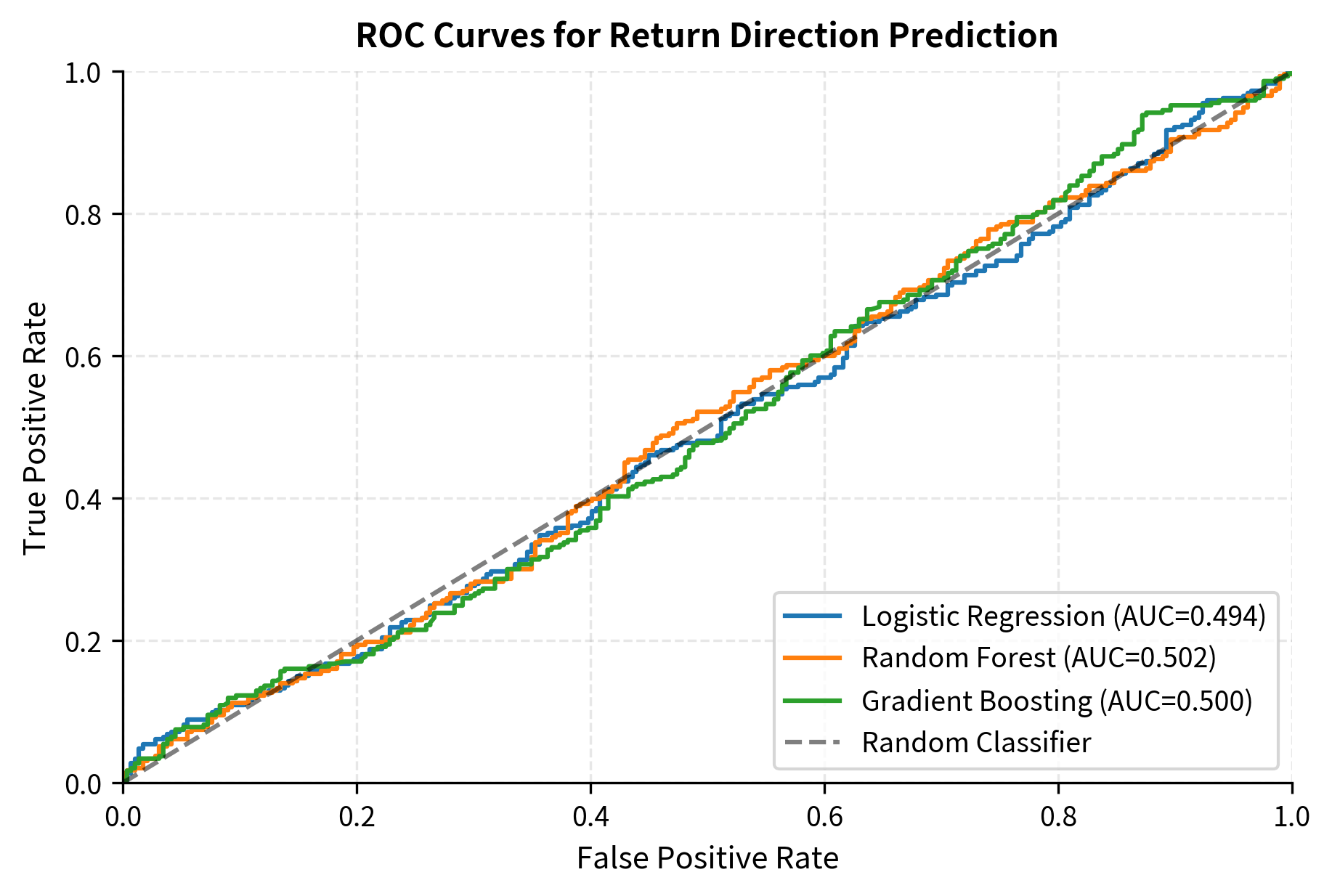
The results reveal a crucial reality of return prediction: accuracy barely exceeds 50%. This isn't a failure of the models or an indication that better algorithms would solve the problem. Instead, it reflects the fundamental difficulty of predicting financial returns. Markets are highly competitive, and any easily exploitable signal gets arbitraged away as sophisticated traders discover and trade on it. The efficient market hypothesis, while not perfectly descriptive, captures an important truth: prices incorporate information quickly, leaving little room for systematic prediction.
The AUC scores slightly above 0.5 indicate that the models capture some genuine predictive information, but the signal-to-noise ratio is extremely low. To put this in perspective, an AUC of 0.52 means that if you randomly select a positive case (day with positive returns) and a negative case, the model ranks the positive case higher only 52% of the time. This slim edge might seem negligible, but when applied consistently across many assets and time periods, even small advantages compound into meaningful returns. The challenge lies in extracting this weak signal reliably without overfitting to noise.
Converting Predictions to Trading Signals
Raw model predictions must be transformed into actionable trading signals before they can generate trades. This transformation step involves deciding not only the direction of trades but also their size and the conditions under which to trade at all. A common approach uses predicted probabilities to determine both direction and position size:
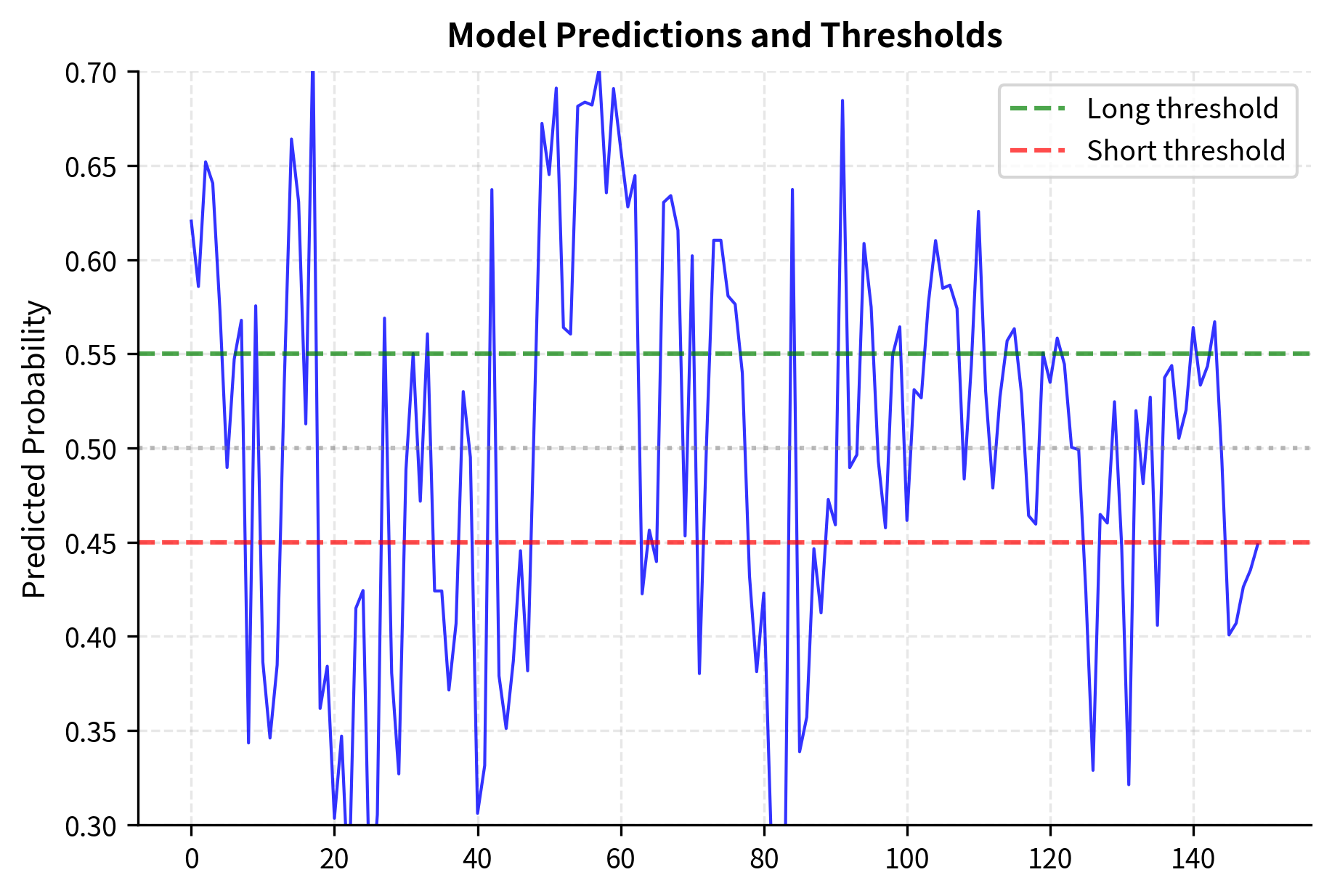
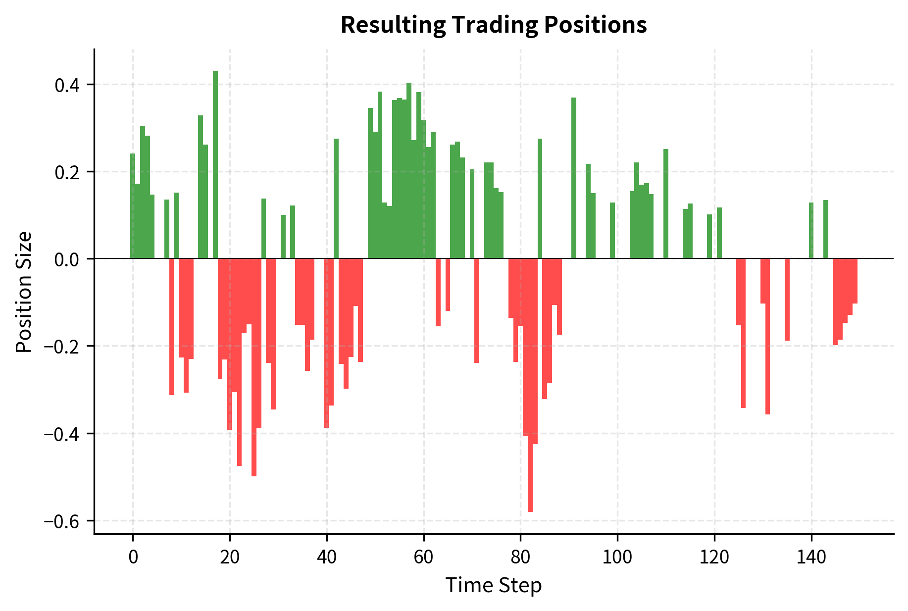
The threshold approach embodies an important principle: not every prediction deserves a trade. By filtering out low-conviction predictions (those close to 50% probability), the strategy only takes positions when the model has sufficient confidence. This filtering serves multiple purposes. It reduces turnover and the associated transaction costs, which can erode returns quickly in frequent-trading strategies. It focuses capital on the highest-quality signals where the model's edge is most pronounced. And it acknowledges the reality that predictions near the decision boundary are essentially random guesses dressed up with spurious precision.
The position sizing component extends this logic further. Rather than taking equal-sized positions regardless of conviction, the strategy scales position size by the model's confidence, measured as the distance from 50%. A prediction of 70% positive return leads to a larger position than a prediction of 56%, reflecting the intuition that stronger signals warrant more capital allocation. This confidence-weighted sizing can significantly improve risk-adjusted returns by ensuring that the portfolio's exposure concentrates in the model's highest-conviction bets.
Evaluating Signal Quality
Beyond classification metrics like accuracy and AUC, we need to evaluate how signals translate into actual trading performance. The connection between prediction quality and trading profit is not straightforward. A model might achieve 55% accuracy, but if its correct predictions tend to coincide with small moves while incorrect predictions coincide with large moves, the trading results could be disappointing.
The information coefficient (IC), which we discussed in Part IV, measures the correlation between predicted and realized returns. This metric directly captures whether the model's signal strength corresponds to return magnitude:
The information coefficient is small but positive, indicating weak but genuine predictive power. Understanding what these numbers mean in context is essential. In the world of trading, even an IC of 0.02 to 0.05 can be valuable when applied across many assets and combined with appropriate leverage. Consider a strategy trading 500 stocks daily: with an IC of 0.03, the model provides a small but consistent edge on each trade that, when aggregated across the entire portfolio, can generate attractive returns.
The profit factor above 1.0 provides complementary information. It tells us that the strategy generates more profit on winning trades than it loses on losing trades. A profit factor of 1.2, for instance, means that for every dollar lost on losing trades, the strategy earns \$1.20 on winning trades. Combined with the hit rate, these metrics paint a complete picture of strategy economics: how often we win, how much we win when we're right, and how much we lose when we're wrong.
Regime-Aware Signal Generation
Market conditions change over time, and a model trained on one regime may fail spectacularly in another. During a strong bull market, momentum strategies thrive as trends persist. During volatile sideways markets, mean-reversion strategies often perform better. A model that doesn't account for these regime shifts will apply momentum signals during ranging markets and mean-reversion signals during trends, suffering losses in both cases.
Regime-aware approaches address this challenge by first identifying the current market state, then adjusting predictions based on the detected regime:
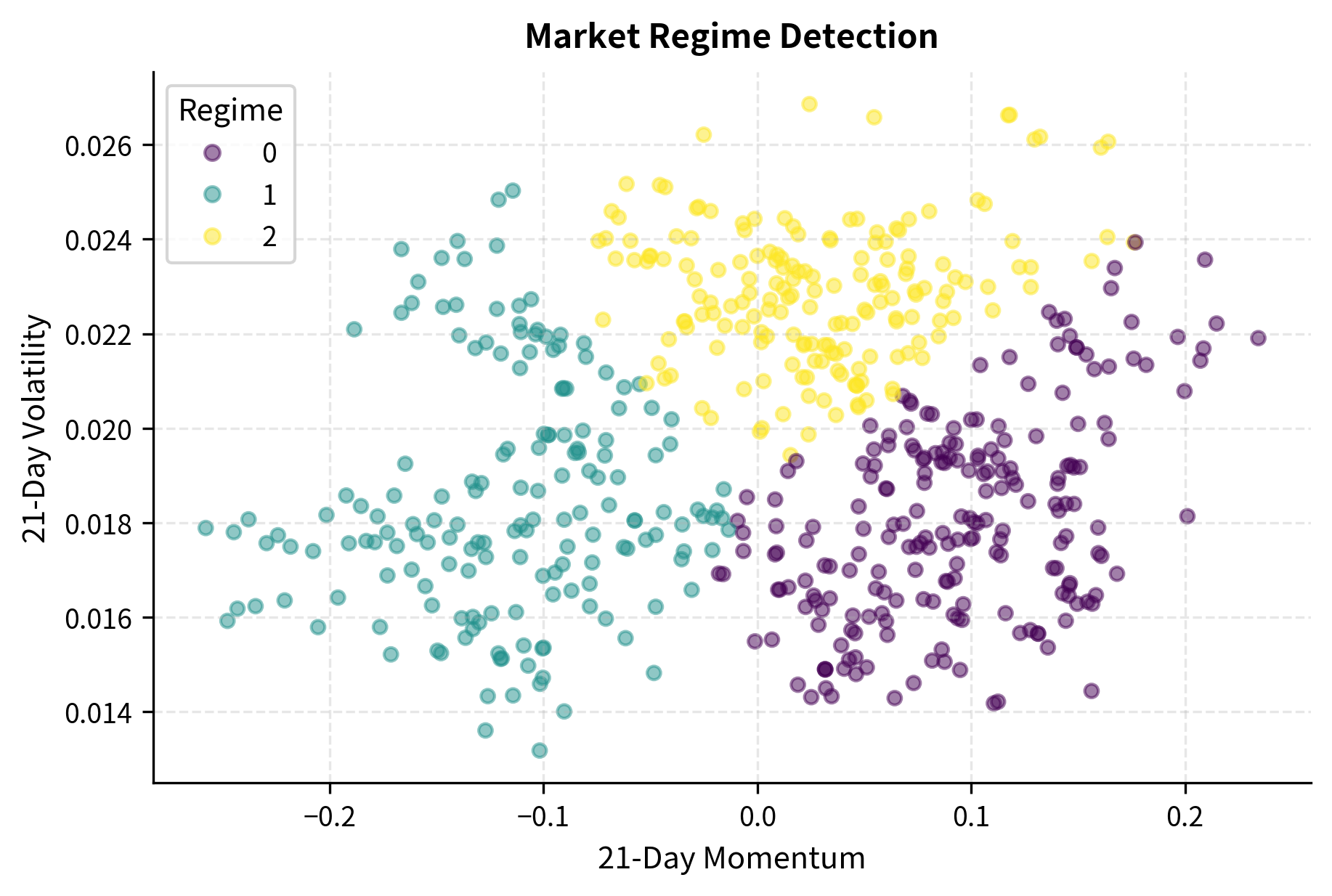
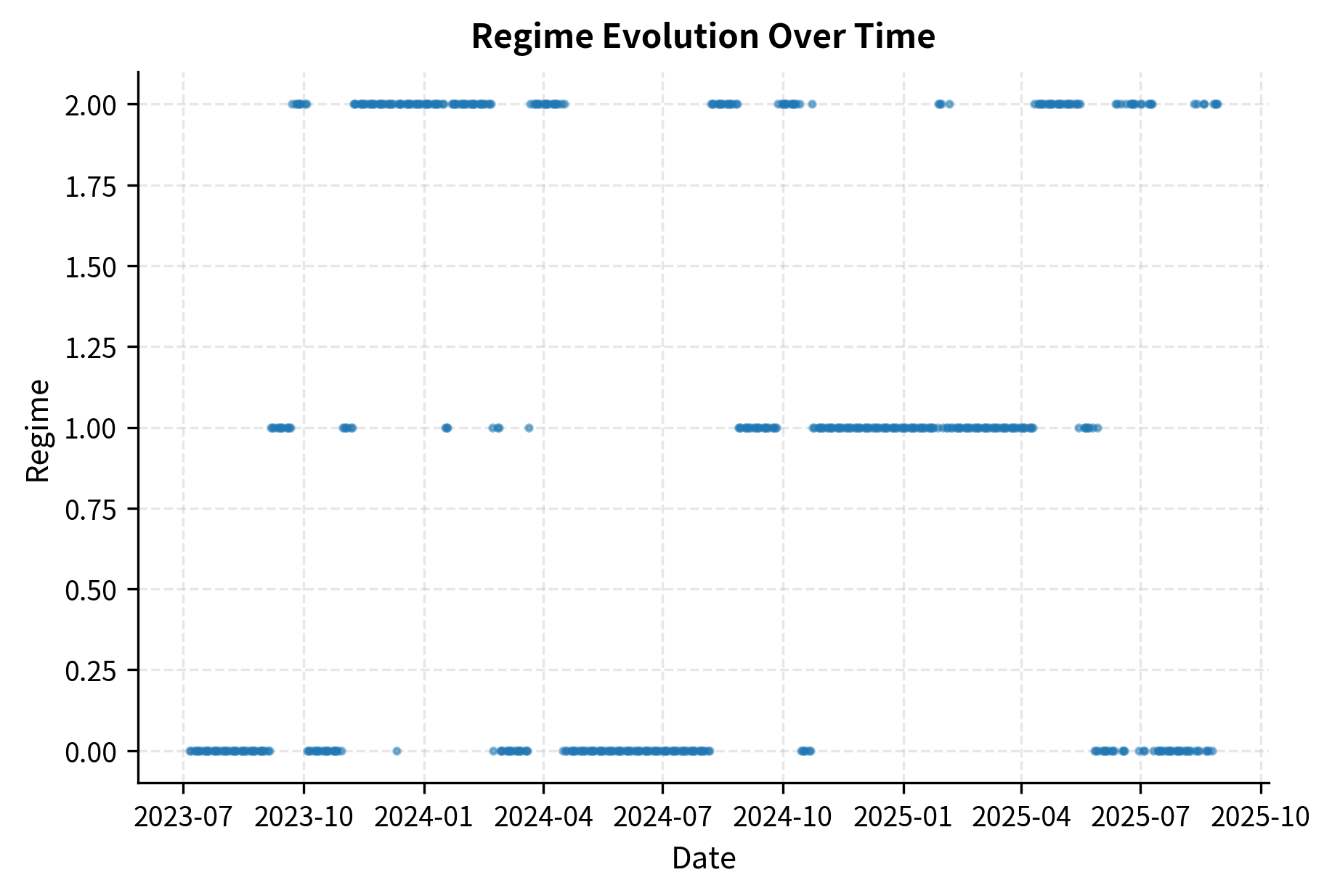
Regime detection enables strategies to adapt their behavior to current market conditions. In practice, you might use momentum signals more aggressively in trending regimes, where past returns have historically predicted future returns, while switching to mean-reversion signals in ranging regimes, where prices oscillate around stable levels. The regime model serves as a meta-layer that conditions the primary prediction model, effectively learning "when" different patterns apply rather than just "what" patterns exist.
The Gaussian Mixture Model approach shown here identifies regimes based on the joint distribution of recent returns and volatility. The three identified regimes typically correspond to distinct market states: calm trending periods with low volatility and consistent directional movement, high-volatility periods often associated with market stress or major uncertainty, and transitional periods that don't fit neatly into either category. By recognizing which regime the market currently occupies, the strategy can apply the most appropriate trading rules for that environment. The next chapter on alternative data explores how external information can improve regime identification beyond what price data alone reveals.
Key Parameters
The key parameters for the supervised learning and regime detection models are:
- n_estimators: The number of trees in the Random Forest or Gradient Boosting model. More trees generally improve stability but increase training time.
- max_depth: The maximum depth of each tree. Constraining depth helps prevent overfitting to noise in financial data.
- learning_rate: Determines the contribution of each tree in Gradient Boosting. Lower rates with more trees often yield better generalization.
- n_components: The number of regimes (clusters) in the Gaussian Mixture Model. This defines how many distinct market states the model attempts to identify.
Sentiment Analysis for Trading Signals
Financial markets are driven not just by fundamentals but by collective psychology. The beliefs, fears, and expectations of market participants manifest in price movements, but they also leave traces in the vast corpus of financial text produced daily. News articles, earnings call transcripts, social media posts, and analyst reports contain information about market sentiment that can predict price movements. Natural language processing (NLP) techniques transform this unstructured text data into quantitative trading signals.
The intuition behind sentiment analysis for trading is straightforward: if we can systematically measure whether market commentary is becoming more optimistic or pessimistic, we might anticipate the buying or selling pressure that follows. When analysts upgrade their tone, when news coverage shifts from concerns to opportunities, when executives speak more confidently on earnings calls, these verbal signals often precede tangible market moves. The challenge lies in converting messy human language into clean numerical signals that trading algorithms can consume.
Text Preprocessing for Financial Data
Financial text requires domain-specific preprocessing. Standard NLP techniques must be adapted to handle ticker symbols, numerical expressions, financial jargon, and the particular ways sentiment is expressed in market contexts. A preprocessing pipeline that works well for movie reviews will struggle with the peculiarities of financial language.
Consider the differences: financial text contains dense numerical information (revenue figures, growth percentages, price targets) that carries meaning. It uses abbreviations and acronyms specific to the industry (EPS, EBITDA, YoY). Ticker symbols appear frequently and must be recognized and associated with their respective companies. Temporal references are crucial, since a statement about "last quarter" means something very different from one about "next fiscal year." These domain-specific features require careful handling:
Preprocessing standardizes the text structure, separating ticker symbols for entity linking and expanding abbreviations to improve consistency across sources. This normalization ensures that the sentiment model focuses on meaningful content rather than formatting variations. Without this step, the same underlying sentiment could appear in many different surface forms, making it harder for the model to learn robust patterns.
Dictionary-Based Sentiment Analysis
The simplest approach to sentiment analysis uses predefined dictionaries of positive and negative words. When encountering text, the algorithm counts occurrences of words from each category and computes a sentiment score based on the balance. Financial-specific dictionaries like Loughran-McDonald are particularly effective because they account for how words carry different connotations in financial versus general contexts.
This domain specificity is crucial. Consider the word "liability": in everyday speech, it's neutral or only mildly negative ("he's a liability to the team"), but in financial contexts, it refers to debts and obligations, carrying a more clearly negative connotation. Similarly, "tax" might be neutral in general text but signals a drag on earnings in financial analysis. Words like "leverage" and "risk" require careful handling, as they can be positive or negative depending on context. General-purpose sentiment dictionaries, trained on movie reviews or product feedback, will misclassify these terms and produce unreliable signals.
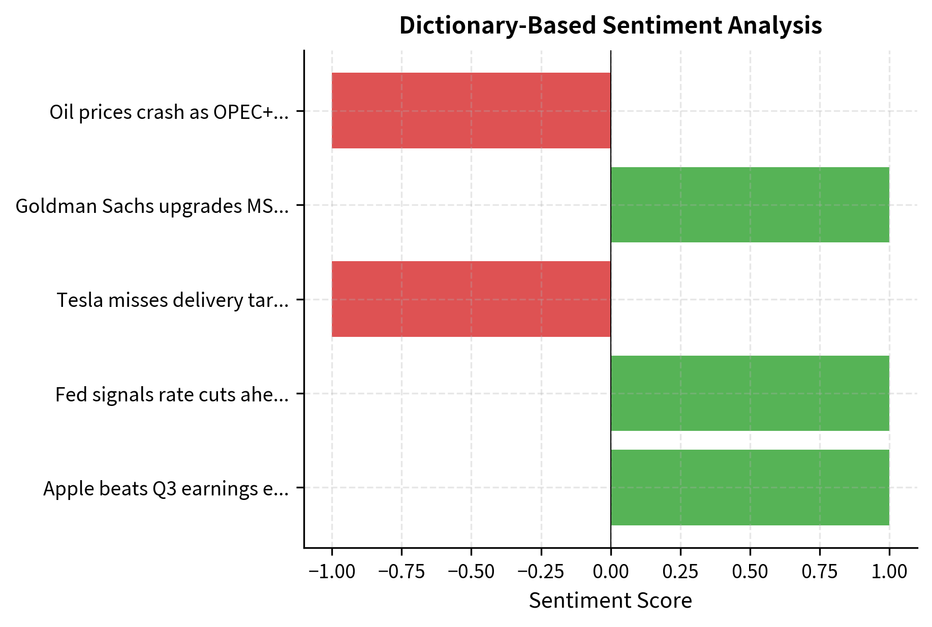
Dictionary-based methods offer important advantages: they are transparent, fast, and require no training data. You can inspect the dictionary and understand exactly how the model reaches its conclusions. This interpretability is valuable for regulatory compliance and internal governance. However, these methods have significant limitations. They miss context entirely. The phrase "not profitable" contains a positive word ("profitable") but expresses negative sentiment through negation. Phrases like "exceeded expectations but guidance disappointed" contain both positive and negative elements that require understanding of sentence structure to interpret correctly. More sophisticated approaches are needed to capture these nuances.
Machine Learning Sentiment Models
Modern sentiment analysis uses machine learning models trained on labeled financial text. These models learn contextual patterns that dictionary methods miss, including negation handling, comparative constructions, and the subtle ways that sentiment is expressed in professional financial communication:
The machine learning model captures nuances that simple keyword matching would miss. By learning from examples of financial text labeled with sentiment, the model develops internal representations that go beyond individual words. It learns that "misses targets" signals negative sentiment even without the word "bad," and that "raises dividend" implies confidence in future cash flows. The TF-IDF vectorization with bigrams helps here, because phrases like "misses targets" or "raises dividend" are captured as single features rather than independent words.
Production sentiment systems typically use more sophisticated architectures, including deep learning models like BERT and its financial variants (FinBERT), which understand context through attention mechanisms that can weigh the importance of different parts of the text. These models can handle complex sentences with multiple sentiment-bearing clauses, correctly parsing constructions like "despite strong revenue growth, margins contracted significantly" as mixed or negative overall.
Aggregating Sentiment Signals
Individual sentiment scores must be aggregated into tradable signals. A single news article provides limited information, but the collective sentiment across all coverage of a company tells a more complete story. Common approaches include time-weighted averages (more recent information matters more), volume-weighted sentiment (high-profile sources like the Wall Street Journal get more weight than obscure blogs), and sentiment momentum (changes in sentiment level):
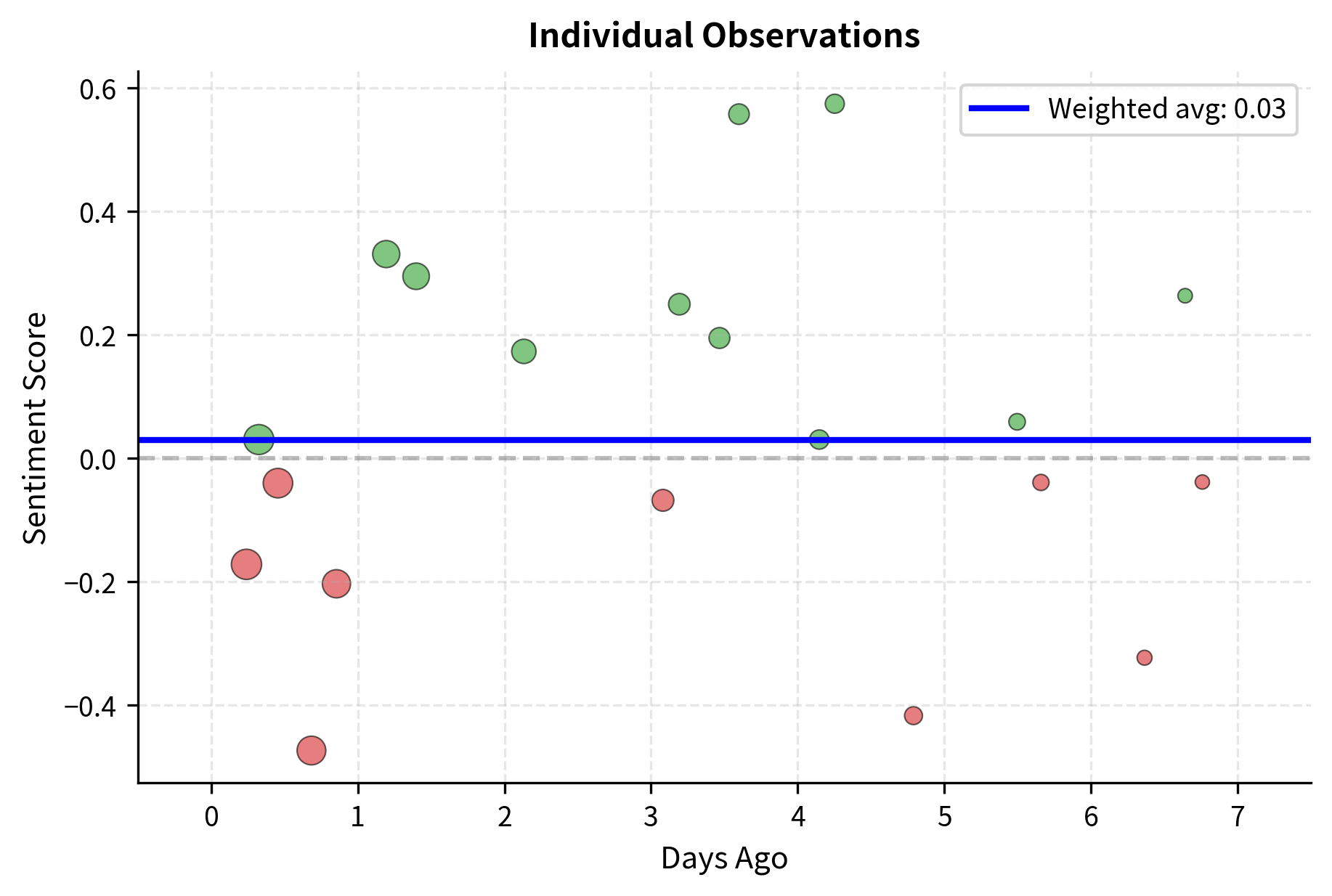
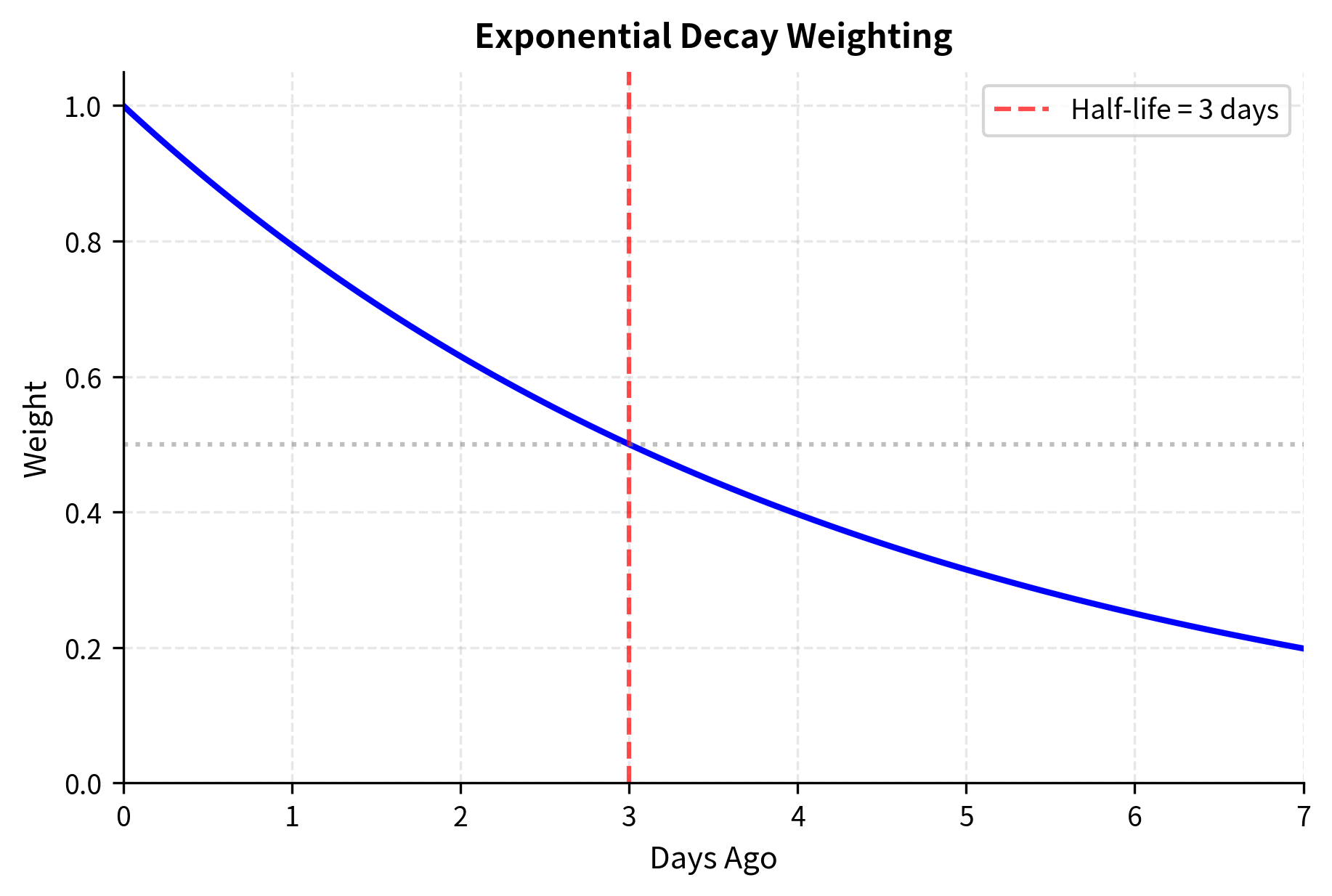
By systematically aggregating signals across multiple sources and time periods, we transform noisy individual data points into a coherent market view. The exponential decay weighting ensures that yesterday's news matters more than last week's, reflecting how information gets incorporated into prices over time. The sentiment dispersion metric captures an often-overlooked dimension: when sources disagree widely, the signal is less reliable than when there's consensus. A stock with uniformly positive coverage provides a stronger buy signal than one with mixed reviews, even if the average sentiment is similar. The momentum component adds yet another layer, capturing whether sentiment is improving or deteriorating. A company with moderately positive sentiment that's improving may be more attractive than one with strongly positive sentiment that's declining.
Key Parameters
The key parameters for the sentiment analysis pipeline are:
- ngram_range: The range of n-grams (word sequences) to extract. Including bigrams (pairs of words) captures context better than single words alone.
- max_features: The maximum number of words to include in the vocabulary. Limiting this focuses the model on the most frequent and informative terms.
- alpha: The smoothing parameter for Naive Bayes. It prevents the model from assigning zero probability to words not seen in the training data.
The next chapter provides a deeper exploration of NLP techniques and alternative data sources, including more sophisticated approaches like transformer-based models and entity extraction.
Alternative Data in Trading Strategies
Alternative data refers to information sources beyond traditional market data and financial statements. Satellite imagery of parking lots, credit card transaction data, web traffic statistics, and shipping container movements can all provide insights into economic activity before it appears in official reports. This data advantage creates alpha when incorporated into trading strategies.
The fundamental insight behind alternative data is that traditional financial metrics, like quarterly earnings reports, are inherently backward-looking and delayed. By the time a company reports revenue growth, the activities generating that revenue occurred weeks or months earlier. Alternative data sources can observe those activities in real-time, providing a preview of what official numbers will eventually show. A fund that can accurately estimate retail sales from credit card data has information that won't appear in public filings for months.
Categories of Alternative Data
Alternative data sources fall into several categories, each with distinct characteristics, coverage, and analytical requirements:
Geospatial data includes satellite and drone imagery used to monitor retail foot traffic, oil storage levels, agricultural yields, and construction activity. A classic example is counting cars in Walmart parking lots to predict quarterly revenue before earnings announcements. Modern computer vision algorithms can automatically process thousands of satellite images daily, counting vehicles, measuring shadow lengths on oil tanks (to estimate fill levels), and assessing crop health from vegetation indices. This data provides direct observation of physical economic activity that eventually flows through to financial statements.
Transaction data encompasses credit card purchases, point-of-sale data, and electronic receipts. These provide real-time views of consumer spending patterns at individual company and sector levels. When a new iPhone launches, credit card data can reveal sales volumes within days, long before Apple reports quarterly results. The granularity is remarkable: analysts can track spending by geography, demographics, and product category. The main limitation is coverage, since any single data provider sees only a fraction of total transactions.
Web and social data includes search trends, app downloads, social media mentions, and website traffic. Surging search interest in a product can predict sales growth, while declining app engagement might signal user attrition before it appears in subscriber counts. Social media sentiment can indicate brand health, customer satisfaction, or emerging crises. Google Trends data, for instance, has been shown to predict earnings surprises for retail companies based on search interest in brand names.
Sensor and IoT data covers supply chain sensors, energy consumption metrics, and industrial equipment monitoring. Real-time shipping data can reveal supply chain disruptions before they impact earnings. Power consumption at manufacturing facilities can indicate production volumes. Fleet tracking data can show logistics efficiency. As more industrial equipment becomes connected, the volume and value of this data category continues to grow.
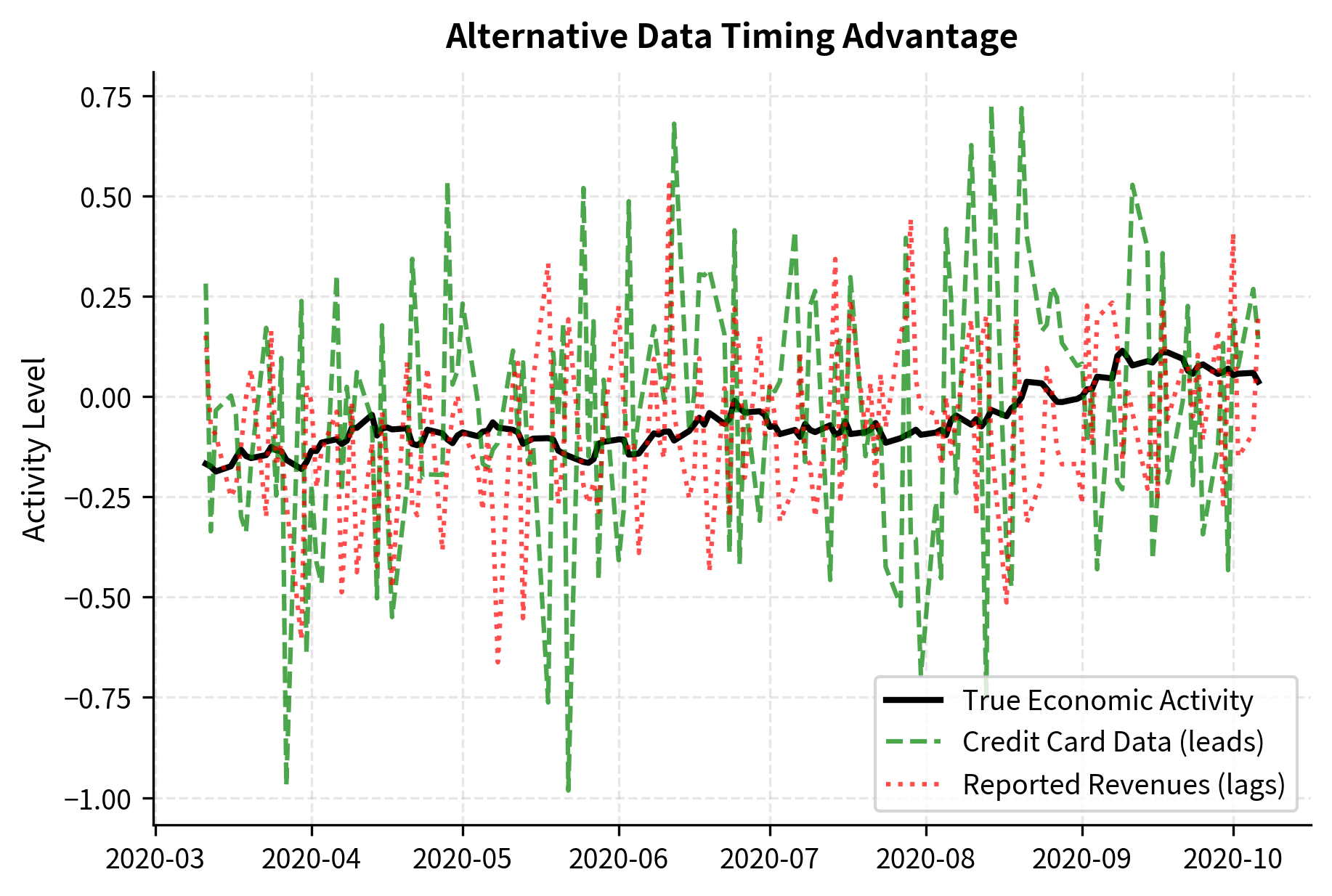
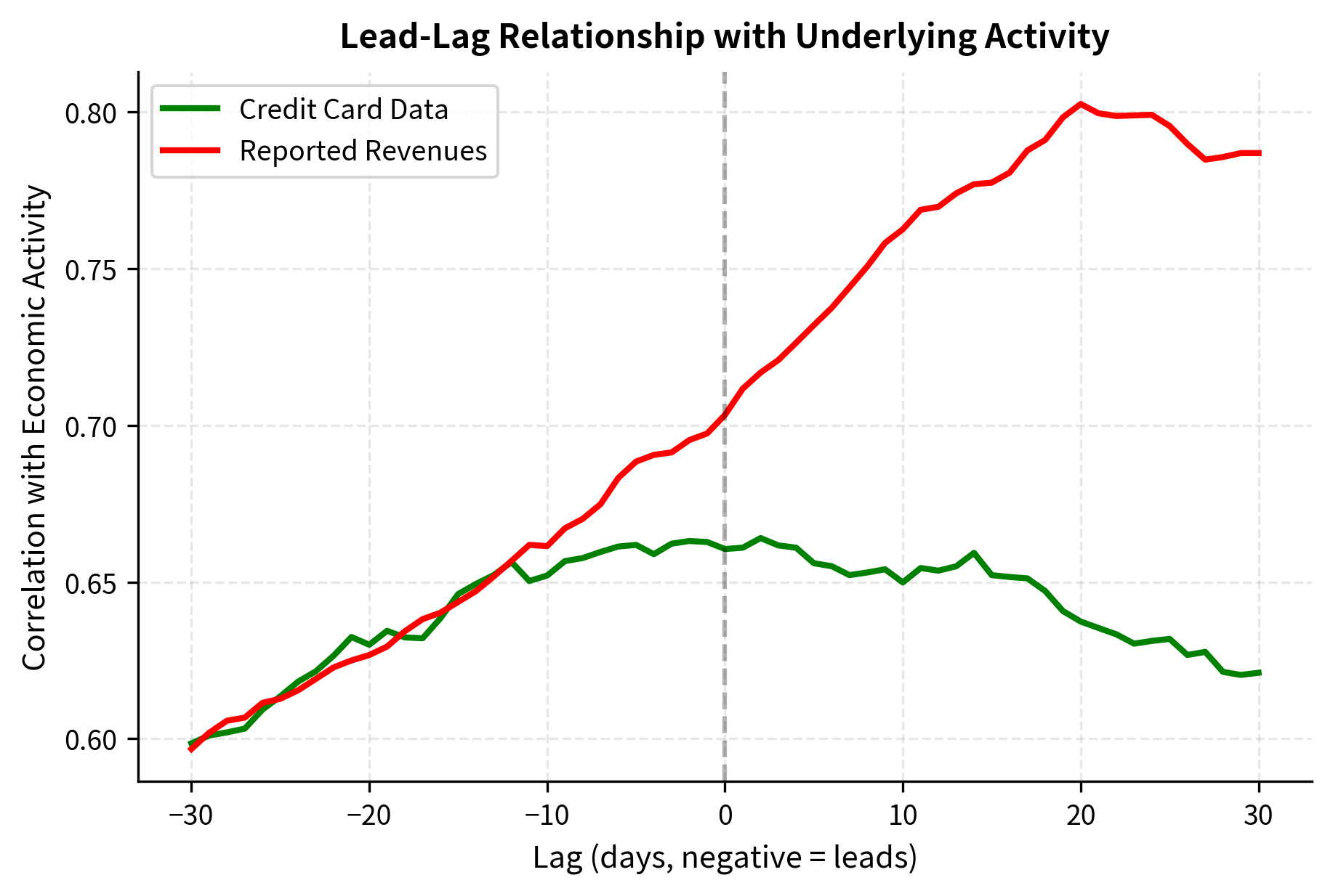
The lead-lag analysis demonstrates visually why alternative data commands premium pricing in the financial industry. Credit card data correlates with economic activity at negative lags, meaning it leads: when we observe credit card spending today, it tells us about economic activity that will be reflected in stock prices over the coming days. Traditional reported data correlates at positive lags, meaning it lags: by the time quarterly revenues are reported, the market has already moved to reflect the underlying activity. This timing advantage can translate into significant trading alpha because you're trading on information that other market participants don't yet have.
Incorporating Alternative Data into Models
Alternative data must be carefully integrated with traditional features. The process involves several key challenges. First, different data sources update at different frequencies: credit card data might be daily, satellite imagery weekly, and reported revenues quarterly. Second, data quality varies dramatically across providers and time periods. Third, there's a significant risk of data snooping: with hundreds of potential alternative data sources, some will appear predictive by chance, and selecting which sources to use based on historical performance can create dangerous overfitting.
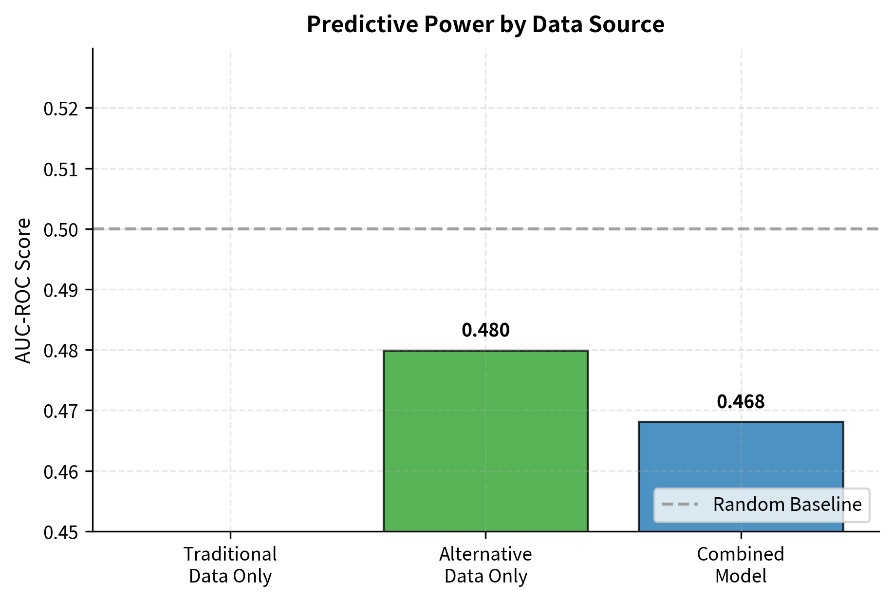
The alternative data model outperforms the traditional data model due to its information timing advantage. By the time traditional metrics are available, much of their informational content has already been reflected in prices. Alternative data captures the same underlying economic activity but with a crucial head start. The combined model often provides incremental improvement over either source alone by capturing both leading signals (from alternative data) and confirming signals (from traditional data). When credit card spending suggests strong sales and reported revenues eventually confirm that strength, the convergence of evidence strengthens conviction.
Key Parameters
The key parameters for integrating alternative data are:
- Lookback Window: The period used for calculating trends and z-scores (e.g., 21 days). This should match the frequency of the alternative data.
- Lag: The time delay applied to align data series. Correctly aligning leading alternative data with lagging market data is critical for extracting alpha.
- n_estimators: The number of trees in the Random Forest. Sufficient trees are needed to capture interactions between alternative and traditional features.
Unsupervised Learning for Market Structure
Not all valuable patterns require labeled data. Unsupervised learning techniques discover hidden structure in market data without being told what to look for. These methods excel at grouping similar assets, identifying regime changes, and detecting anomalies that signal risk or opportunity. The absence of labels forces these algorithms to find patterns based on the intrinsic structure of the data, often revealing relationships that wouldn't be apparent from traditional analysis.
Clustering for Portfolio Construction
Hierarchical clustering and k-means provide data-driven alternatives to traditional sector classifications. Standard industry categories, like GICS sectors or NAICS codes, group companies based on what they do. But for portfolio construction, what matters is how assets behave together in the market, their return correlations and factor exposures. Two tech companies in the same GICS sector might have very different risk profiles if one is a growth stock sensitive to interest rates while the other is a mature value play.
Assets grouped by return covariance patterns may reveal economic relationships that standard industry categories miss. A cloud computing company might cluster more closely with commercial real estate (both sensitive to business investment cycles) than with social media companies (more dependent on advertising spending). By letting the data determine groupings, clustering can identify these unexpected but economically meaningful relationships:
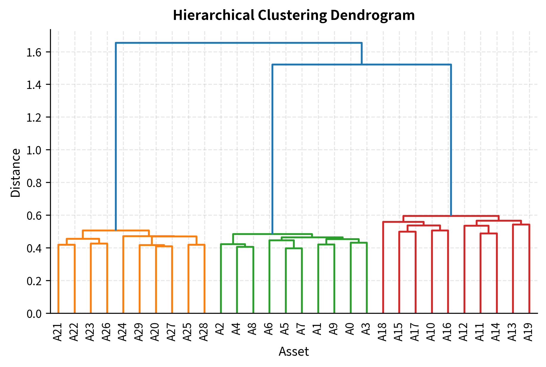
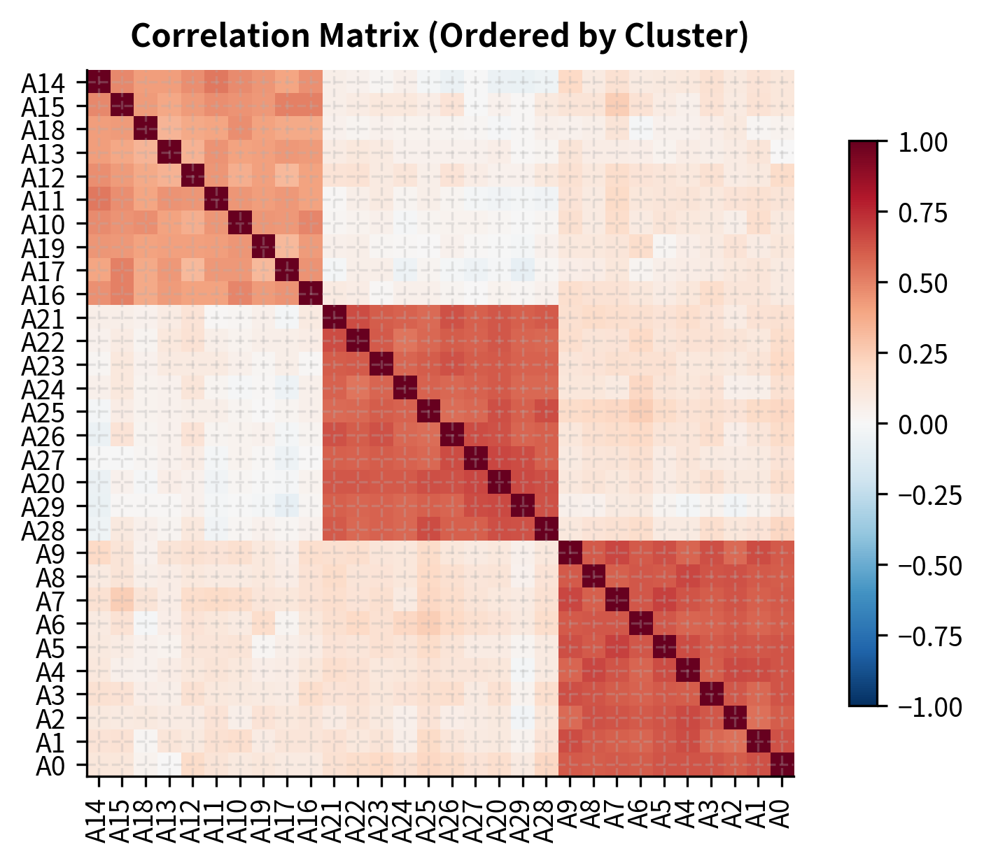
The clustering identifies natural groupings in the data that can inform portfolio construction. The dendrogram on the left shows the hierarchical structure of asset relationships: assets that merge at lower heights are more similar, while those that only join at the top of the tree are quite different. The correlation heatmap on the right, reordered by cluster membership, reveals the block structure that clustering uncovers. Within each block (cluster), correlations are high, indicating that these assets move together. Between blocks, correlations are lower, suggesting genuine diversification potential.
Rather than using arbitrary sector classifications that may not reflect current market dynamics, you can build diversified portfolios by selecting assets from different clusters. This approach ensures genuine diversification of risk exposures based on how assets actually behave, not how they're categorized. When correlations change (as they often do during market stress), the clusters can be recomputed to maintain effective diversification.
Anomaly Detection for Risk Management
Unsupervised anomaly detection identifies unusual market behavior that might signal emerging risks or trading opportunities. The logic is that normal market conditions, while noisy, exhibit statistical regularities. When these regularities break down, when volatility spikes unexpectedly, when correlations shift dramatically, when the distribution of returns changes character, something unusual is happening. Detecting these anomalies early can help traders manage risk or capitalize on dislocations.
Isolation forests and autoencoders are particularly effective for high-dimensional financial data. Isolation forests work by recursively partitioning data; points that can be isolated quickly (with few partitions) are anomalous because they're far from the dense regions where most data lies. This approach is computationally efficient and doesn't require assumptions about the distribution of normal data:
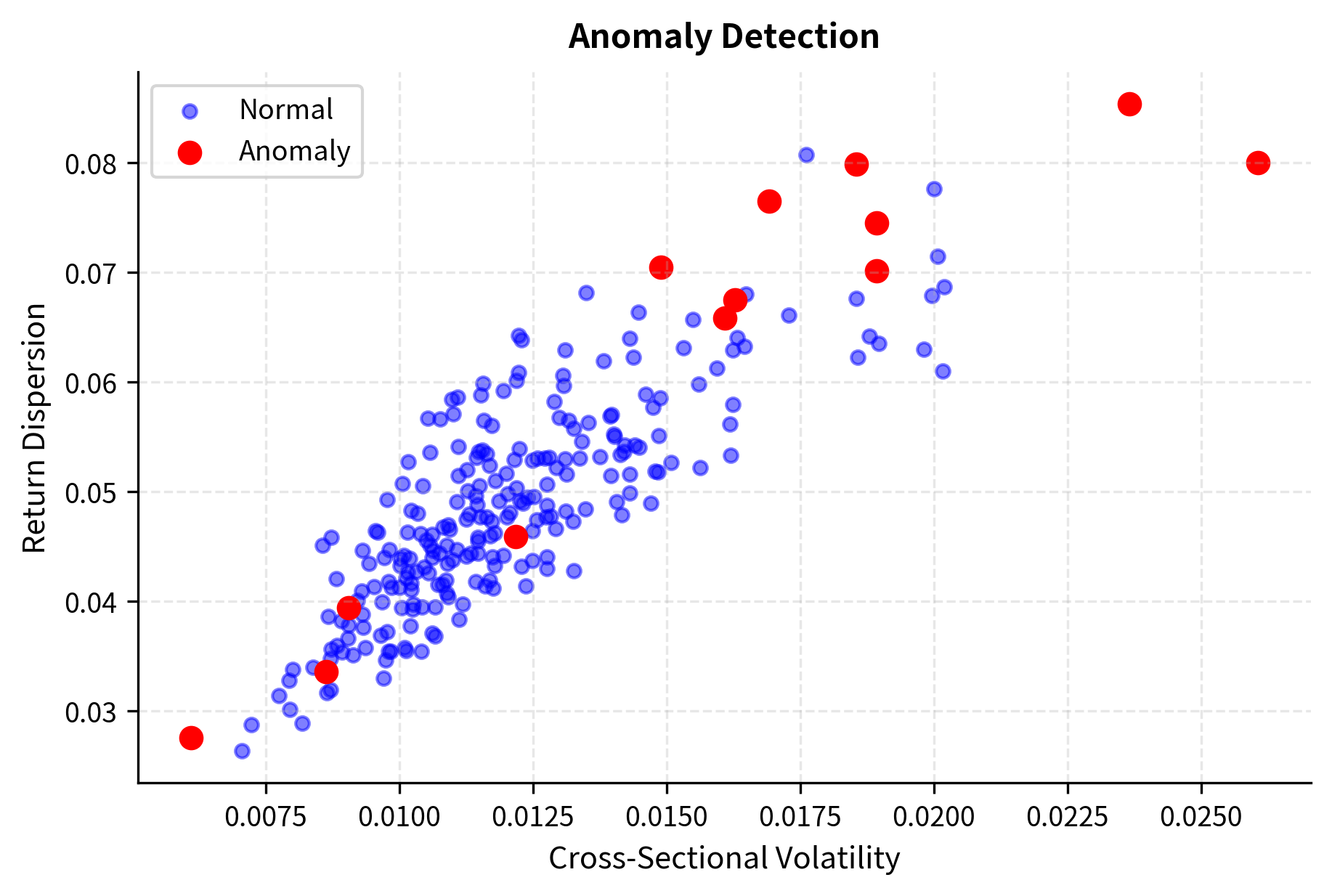
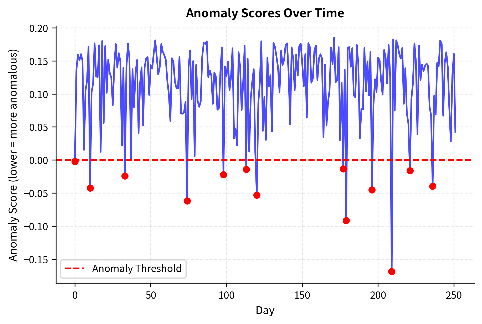
The visualization highlights how the model isolates days with extreme cross-sectional properties. Normal market behavior (blue points) clusters in a characteristic region of the volatility-dispersion space. Anomalous days (red points) appear in unusual locations: perhaps extremely high volatility with moderate dispersion (a correlated sell-off), or moderate volatility with extreme dispersion (a sector rotation with some stocks surging while others crash). Each anomaly pattern tells a different story about what's happening in the market.
Anomaly detection serves multiple purposes in trading. It can identify potential market dislocations that create trading opportunities, since unusual conditions often precede mean-reversion. It can flag unusual portfolio behavior that warrants risk review, alerting managers when their positions are experiencing statistically unusual moves. And it can detect data quality issues before they corrupt model inputs, catching feed errors or stale prices that might otherwise trigger erroneous trades.
Key Parameters
The key parameters for unsupervised market structure models are:
- n_clusters: The number of groups to find in K-Means clustering. This determines the granularity of the resulting asset universe.
- contamination: The expected proportion of anomalies in the dataset for Isolation Forest. This sets the threshold for flagging data points as outliers.
- linkage: The method used to calculate distances between clusters in hierarchical clustering (e.g., 'ward'). Different methods produce different cluster shapes.
Reinforcement Learning in Trading
Reinforcement learning (RL) offers a fundamentally different approach to trading strategy design. Rather than predicting returns directly and then deciding how to trade based on those predictions, RL agents learn optimal actions through trial and error, maximizing cumulative reward over time. This framework naturally handles the sequential nature of trading decisions, where today's action affects tomorrow's opportunities. It also directly incorporates transaction costs, market impact, and position constraints that complicate traditional predict-then-optimize approaches.
The key insight motivating RL for trading is that maximizing prediction accuracy doesn't necessarily maximize trading profit. A model might be very accurate at predicting small moves but miss the occasional large move that dominates returns. RL sidesteps this issue by optimizing the ultimate objective (cumulative risk-adjusted returns) rather than an intermediate proxy (prediction accuracy).
The RL Framework for Trading
To understand how RL applies to trading, consider the core components of any RL problem. A trading problem formulated as RL has three key elements:
State : This represents all the information available to the agent at time for making decisions. In trading, the state typically includes current market information such as recent prices, volumes, and technical indicators. It also includes the agent's current position, which affects what actions are feasible and desirable. Additional features might include sentiment scores, alternative data signals, or estimates of market impact.
Action : This is the trading decision made at each time step. Actions might be discrete, such as buy, sell, or hold, or they might be continuous, representing a target position size or the fraction of capital to allocate. The action space design significantly affects learning difficulty: discrete actions are simpler but may miss nuance, while continuous actions are more flexible but harder to optimize.
Reward : This is the feedback signal that guides learning. Unlike supervised learning where labels are provided, RL agents discover what's good through reward signals. For trading, natural reward choices include raw returns, risk-adjusted returns (Sharpe-like measures), or utility functions that penalize drawdowns. The reward design encodes what you're optimizing for: a reward based on raw returns encourages aggressive risk-taking, while a Sharpe-based reward balances returns against volatility.
The agent learns a policy that maps states to actions, maximizing the expected cumulative discounted reward. The objective function is:
where:
- : expected cumulative reward under policy
- : expectation operator over trajectory distributions
- : terminal time step
- : current time step
- : discount factor ()
- : reward received at time
The discount factor balances the importance of immediate rewards against long-term gains. A close to 1 makes the agent patient, willing to sacrifice immediate profits for larger future rewards. A lower makes the agent more myopic, focusing on near-term results. For most trading applications, is set close to 1 (e.g., 0.95-0.99) because we care about long-term cumulative returns.
Q-Learning for Trading
Among the many RL algorithms, Q-learning provides an intuitive foundation for understanding how agents learn to trade. Q-learning learns the action-value function , which estimates the expected cumulative reward from taking action in state and following the optimal policy thereafter. The "Q" in Q-learning stands for "quality," representing how good it is to take a particular action in a particular state.
For continuous states like those in trading (where features are real-valued), we cannot store Q-values in a table as we might for simple games. Instead, we approximate with a function approximator. In the example below, we use a simple linear function; in production systems, deep neural networks create Deep Q-Networks (DQN) that can capture complex nonlinear relationships:
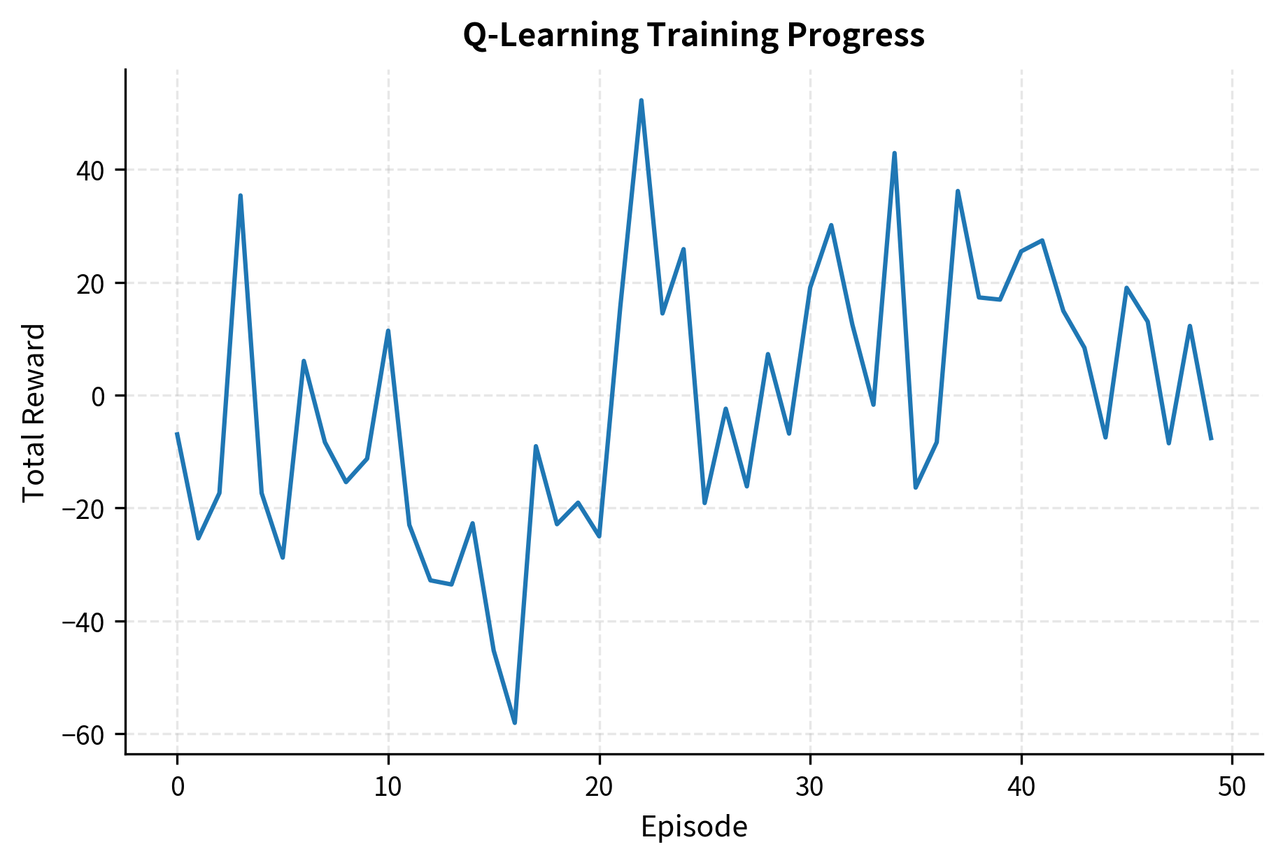
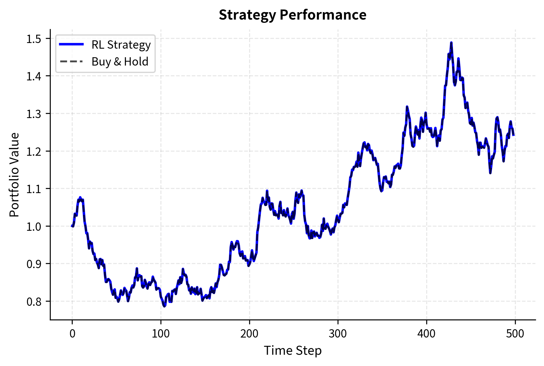
The training curves illustrate the learning process. Early episodes show high variance as the agent explores randomly (high epsilon), taking many suboptimal actions to gather information about the environment. As training progresses and epsilon decays, the agent increasingly exploits its learned knowledge, and cumulative rewards stabilize at higher levels. The strategy performance comparison on the right demonstrates that the trained agent can outperform a simple buy-and-hold approach by timing entries and exits based on market features. When momentum is positive, the agent learns to hold long positions; when momentum turns negative, it either exits or goes short.
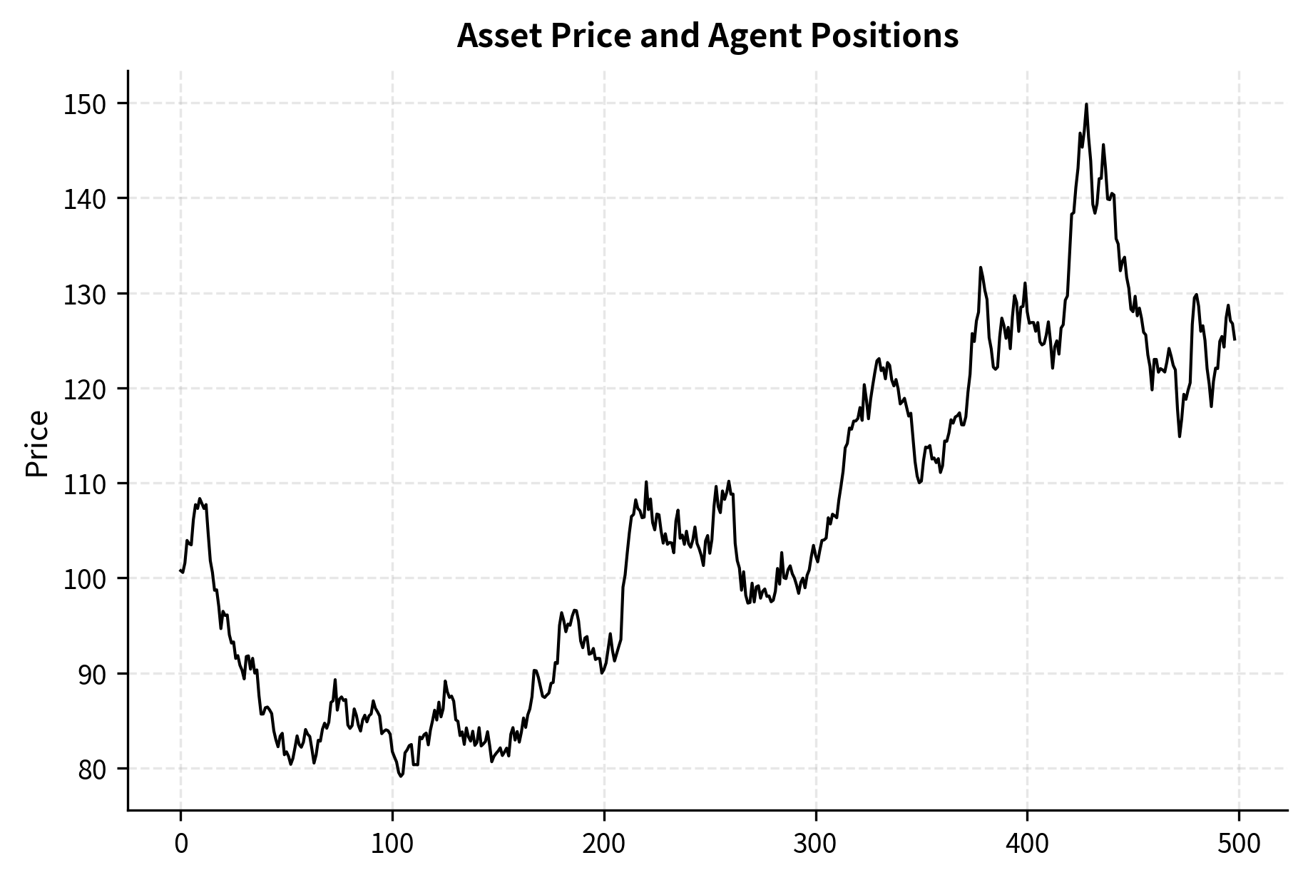
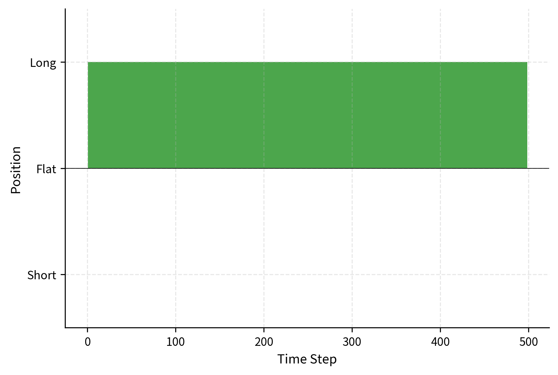
The RL strategy achieves a higher Sharpe ratio than the buy-and-hold benchmark, indicating better risk-adjusted returns. This improvement comes from two sources. First, by going flat or short during periods of negative momentum, the agent avoids some drawdowns that the buy-and-hold strategy suffers. Second, the agent concentrates its exposure during favorable periods, capitalizing on momentum when signals are strong. The lower volatility of the RL strategy reflects this more selective approach to market exposure. Despite the transaction costs incurred from position changes, the risk management benefit outweighs the friction.
Key Parameters
The key parameters for the Q-learning agent are:
- learning_rate: Controls how much new information overrides old information. In noisy markets, a lower rate helps average out stochastic rewards.
- discount_factor (): Determines the importance of future rewards. A value close to 1 makes the agent farsighted, while a lower value focuses on immediate returns.
- epsilon (): The probability of choosing a random action (exploration). Decaying this value over time allows the agent to exploit its learned policy.
Applications of RL in Trading
Reinforcement learning excels in several trading applications where the sequential nature of decisions and the need to balance multiple objectives make traditional approaches awkward:
Optimal execution involves minimizing market impact when executing large orders. A fund that needs to buy a million shares faces a dilemma: trading quickly risks moving the market against itself, but trading slowly exposes the position to adverse price drift. The RL agent learns to balance urgency (completing the order quickly) against market impact (moving the price adversely), adapting its strategy to real-time market conditions like volatility and liquidity. This is explored further in Part VII when we cover execution algorithms.
Dynamic portfolio rebalancing uses RL to decide when and how much to rebalance, accounting for transaction costs, tax implications, and changing market conditions. Unlike fixed-schedule rebalancing (e.g., monthly on the first trading day), RL-based approaches adapt to market volatility and opportunity costs. When drift is small and costs are high, the agent learns to delay rebalancing; when positions have moved substantially or volatility has spiked, it learns to act quickly.
Market making benefits from RL's ability to learn optimal quote placement strategies that balance inventory risk against spread capture. The market maker's challenge is to profit from the bid-ask spread while avoiding accumulating large positions that expose it to directional risk. The agent learns when to widen spreads (during high volatility or low liquidity) and when to compete aggressively for order flow (in calm markets with balanced two-sided demand).
- Non-stationarity: Markets change over time, invalidating learned policies
- Sparse rewards: Meaningful feedback (annual returns) requires long episodes
- Simulation fidelity: Training environments may not capture real market dynamics
- Sample efficiency: RL requires many interactions, but historical data is limited
Practical Challenges and Model Governance
Deploying ML models in live trading requires addressing challenges that don't appear in research settings: overfitting to historical data, model interpretability for risk management, and the infrastructure needed for real-time prediction.
Overfitting and Generalization
The fundamental challenge of ML in trading is that financial relationships are weak and change over time. Standard cross-validation overestimates performance because it ignores temporal structure: by mixing future data into training folds, it allows the model to learn patterns that wouldn't be available in real trading. We covered time-series cross-validation in the previous chapter; here we examine additional techniques for robust evaluation that more faithfully simulate the deployment environment:
#| echo: false #| output: true #| fig-cap: "Walk-forward validation AUC scores across sequential test periods. The green bars (AUC > 0.5) and red bars (AUC < 0.5) visualize performance stability. The variability, with some periods falling below the random baseline, highlights the non-stationarity of financial markets and the risks of relying on static models." #| fig-file-name: walk-forward-validation-results
import matplotlib.pyplot as plt
plt.rcParams.update({ "figure.figsize": (6.0, 4.0), # Adjust for layout "
Quiz
Ready to test your understanding? Take this quick quiz to reinforce what you've learned about machine learning in trading strategy design.

Comments