

Learn supervised ML algorithms for trading: linear models, random forests, gradient boosting. Master feature engineering and cross-validation to avoid overfitting.
Choose your expertise level to adjust how many terms are explained. Beginners see more tooltips, experts see fewer to maintain reading flow. Hover over underlined terms for instant definitions.
Machine Learning Techniques for Trading
The systematic trading strategies we have explored throughout Part VI, including mean reversion, momentum, factor investing, and volatility trading, all rely on identifying patterns in financial data. Traditionally, you specified these patterns explicitly through carefully crafted rules and statistical models. Machine learning offers a fundamentally different approach: rather than specifying the patterns, we let algorithms discover them directly from data.
This shift has profound implications for quantitative finance. Machine learning can process vastly more features than a human analyst could reasonably manage, detect nonlinear relationships that elude traditional regression models, and adapt to changing market conditions through regular retraining. At the same time, the application of ML to financial markets presents unique challenges that don't exist in other domains like image recognition or natural language processing. Markets are adversarial, returns are noisy with low signal-to-noise ratios, and the statistical properties of financial data shift over time.
This chapter introduces the core machine learning techniques used in quantitative trading, with particular emphasis on the methodological rigor required to avoid the many pitfalls that await you. We'll cover the major classes of learning algorithms, the art of transforming raw market data into predictive features, and the validation techniques essential for building models that generalize to unseen data rather than merely memorizing historical patterns.
The Machine Learning Landscape in Finance
Machine learning encompasses a broad family of algorithms that learn patterns from data. These methods are typically categorized by the nature of the learning task and the type of supervision provided during training.
Supervised Learning
In supervised learning, we have labeled training data consisting of input features and corresponding target values . The goal is to learn a function that maps inputs to outputs, enabling predictions on new, unseen data. In finance, supervised learning addresses two primary tasks:
- Regression: Predicting continuous values such as future returns, volatility, or prices. For example, forecasting next-day returns based on technical indicators.
- Classification: Predicting categorical outcomes such as the direction of price movement (up/down), whether a company will default, or whether an earnings announcement will beat expectations.
Building on the regression analysis from Part III, supervised learning extends these ideas with more flexible functional forms that can capture complex, nonlinear relationships.
Unsupervised Learning
Unsupervised learning works with unlabeled data, seeking to discover hidden structure without explicit targets. Common applications in finance include:
- Clustering: Grouping similar assets, trading regimes, or market conditions. K-means clustering might identify stocks with similar return characteristics, while regime detection algorithms could classify market states (trending, mean-reverting, high-volatility).
- Dimensionality Reduction: Compressing high-dimensional data into fewer factors. As we covered in Part III when discussing Principal Component Analysis, this helps identify latent factors driving asset returns and reduces computational complexity.
- Anomaly Detection: Identifying unusual observations such as potential fraud, data errors, or market dislocations.
Reinforcement Learning
Reinforcement learning involves an agent learning to make sequential decisions through trial and error, receiving rewards based on the outcomes of its actions. This framework is conceptually appealing for trading: the agent (trading system) takes actions (trades) in an environment (market) and receives rewards (profits or losses). However, reinforcement learning faces significant challenges in finance due to the non-stationarity of markets, the need for extensive exploration (which is costly in real markets), and the difficulty of defining appropriate reward functions. While active research continues, supervised learning remains the dominant paradigm for most practical quantitative trading applications.
Supervised Learning Algorithms
Let's examine the supervised learning algorithms most commonly employed in quantitative finance, building from simple linear models to more complex ensemble methods and neural networks.
Linear and Logistic Regression Revisited
Linear regression, which we covered extensively in Part III's chapter on regression analysis, remains a foundational tool. The intuition behind linear regression is straightforward: we assume that the target variable can be expressed as a weighted sum of the input features, plus some random noise that captures everything our model cannot explain. This assumption, while restrictive, proves remarkably useful in many financial applications where relationships between variables are approximately linear over relevant ranges.
For predicting continuous targets like returns, we model:
where:
- : dependent variable (target)
- : y-intercept
- : regression coefficient for feature
- : independent variable (feature)
- : total number of features
- : error term (residual)
To understand what this formula truly represents, consider each coefficient as quantifying the expected change in the target variable when feature increases by one unit, holding all other features constant. The intercept captures the baseline prediction when all features equal zero. The error term acknowledges that our linear model cannot perfectly explain every observation; it represents the inherent randomness in financial markets and the influence of factors we have not included.
Despite its simplicity, linear regression offers important advantages: interpretability, computational efficiency, and well-understood statistical properties. Its coefficients tell us exactly how each feature influences the prediction. When a portfolio manager asks why the model is bullish on a particular stock, we can point to specific features and their associated weights, providing a clear narrative that connects inputs to outputs.
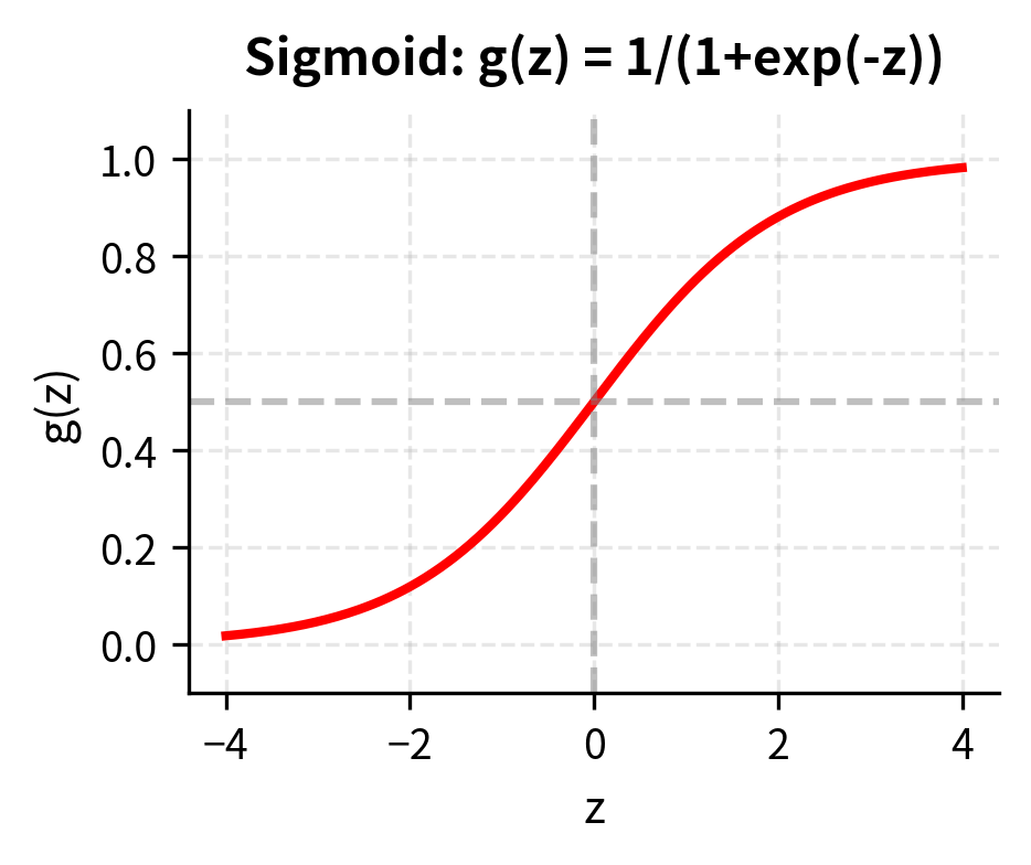
For binary classification tasks, such as predicting whether returns will be positive or negative, we need a different approach. The challenge is that linear regression produces unbounded outputs, yet we need probabilities that fall between zero and one. Logistic regression solves this elegantly by wrapping the linear combination inside a special transformation called the logistic (or sigmoid) function. Logistic regression models the probability of the positive class:
where:
- : probability of the positive class given features
- : the log-odds (linear combination) of the features
- : bias term
- : vector of weights
- : vector of input features
The logistic function performs a crucial transformation. Inside the exponential, we still have our familiar linear combination of features. However, the logistic function squashes this linear combination into the interval, giving us probability estimates rather than unbounded predictions. When the linear combination is large and positive, the probability approaches 1; when it is large and negative, the probability approaches 0; and when the linear combination equals zero, the probability equals exactly 0.5.
![The logistic (sigmoid) function across the range [-6, 6]. The curve squashes real-valued inputs into the (0, 1) interval, with the steepest gradient and decision boundary occurring at z = 0.](https://cnassets.uk/notebooks/8_ml_techniques_files/gradient-boosting-staged-loss.png)
The coefficients reveal the relationship between features and targets. Momentum shows a positive relationship with returns (as expected from our data generation), while the mean reversion signal has a negative coefficient, consistent with the contrarian nature of mean reversion strategies.
Key Parameters
- fit_intercept: Whether to calculate the intercept (bias) term. In finance, this represents the alpha or base probability.
- C: Inverse of regularization strength for logistic regression (default 1.0). Smaller values specify stronger regularization to prevent overfitting.
- penalty: The norm used in the penalization (e.g., 'l2').
Decision Trees
Decision trees partition the feature space through a sequence of binary splits, creating a hierarchical structure that naturally captures nonlinear relationships and feature interactions. The fundamental idea is intuitive: at each step, the algorithm asks a yes-or-no question about one of the features (such as "Is momentum greater than 0.5?"), and based on the answer, it routes the observation down one of two branches. This process continues recursively until the observations reach terminal nodes, called leaves, where the final prediction is made.
At each internal node, the tree selects a feature and threshold that best separates the data according to some criterion. For classification tasks, this criterion is typically Gini impurity while for regression tasks, mean squared error is commonly used. This approach automatically discovers which features matter most and identifies the thresholds that create the most informative splits.
Gini impurity provides a measure of how often a randomly chosen element would be incorrectly classified if we assigned labels according to the distribution of classes in that node. Intuitively, a node where all observations belong to a single class is "pure" and has zero impurity, while a node with an even mix of classes has maximum impurity.
For a node with class probabilities , the Gini impurity is:
where:
- : Gini impurity measure
- : probability of class
- : total number of classes
Pure nodes (all one class) have .
To see why this formula makes sense, consider a binary classification problem. If a node contains only positive examples (), then , indicating perfect purity. Conversely, if the node contains an equal mix (), then , the maximum possible impurity for two classes.
The tree-building process recursively finds the optimal split at each node by evaluating all possible features and thresholds, selecting the combination that most reduces the weighted impurity of the resulting child nodes:
where:
- : feature index selected for the split
- : threshold value for feature
- : left and right child nodes
- : number of samples in the left and right child nodes
- : total number of samples in the current node
- : function measuring node impurity (e.g., Gini)
This formula captures the essence of the splitting decision. We weight each child node's impurity by the proportion of samples it receives, ensuring that we prioritize splits that create large, pure groups rather than small pockets of purity. The algorithm searches over all features and all possible thresholds to find the combination that minimizes this weighted impurity.
Random forests improve on individual decision trees by training an ensemble of trees, each on a bootstrapped sample of the data with a random subset of features considered at each split. The core insight draws from a fundamental principle in statistics: while individual estimates may be noisy, averaging many independent estimates reduces that noise.
Consider the variance reduction that comes from averaging. If we have independent predictions, each with variance , their average has variance . Of course, trees trained on the same data are not truly independent. This is where the clever design of random forests comes into play. By introducing randomness in both the data (bootstrap sampling) and features (random feature subsets at each split), the individual trees become decorrelated. Even though each tree may be a somewhat biased estimator of the true function, their average prediction is more stable than any single tree could achieve.
The final prediction aggregates across all trees:
where:
- : aggregated ensemble prediction
- : total number of trees in the forest
- : prediction generated by the -th tree
- : input feature vector
For classification tasks, this aggregation typically takes the form of majority voting: each tree casts a vote for its predicted class, and the class receiving the most votes becomes the ensemble prediction. For regression, we simply average the numerical predictions. The key insight is that averaging reduces variance without increasing bias. By introducing randomness in both the data (bootstrap sampling) and features (random feature subsets), the individual trees become decorrelated, and their average prediction is more stable than any single tree.
Random forests are remarkably robust and require relatively little hyperparameter tuning. They handle mixed feature types, provide probability estimates through voting, and offer feature importance measures. Their main limitations are computational cost (training many trees) and reduced interpretability compared to single trees.
Key Parameters
- n_estimators: The number of trees in the forest. More trees increase stability but also computational cost.
- max_depth: The maximum depth of each tree.
- max_features: The number of features to consider when looking for the best split.
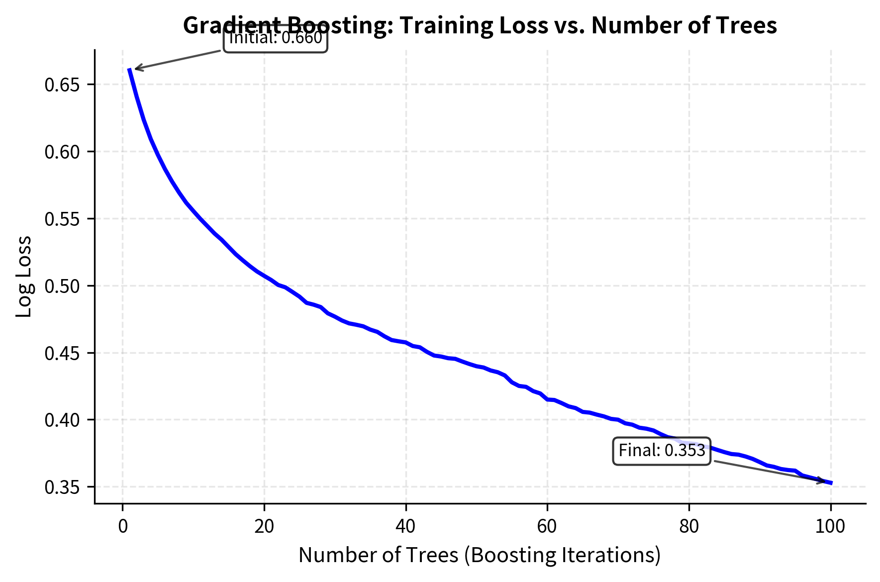
Gradient Boosting
While random forests build trees independently and average their predictions, gradient boosting takes a fundamentally different approach by building trees sequentially, with each tree correcting the errors of the previous ensemble. The conceptual difference is significant: random forests reduce variance through averaging, while gradient boosting reduces bias through iterative refinement.
The method works by fitting each new tree to the negative gradient of the loss function. To understand this intuitively, think of the gradient as pointing in the direction of steepest ascent. By moving in the opposite direction (the negative gradient), we descend toward lower loss values. In the case of squared error loss, this negative gradient equals the residuals, the differences between actual values and current predictions. In essence, each new tree learns to predict the mistakes of the ensemble so far.
For regression with squared error loss, the algorithm proceeds in steps:
- Initialize with the mean value:
where:
- : initial prediction (mean value)
- : mean of the target values
- : input feature vector
Starting with the mean is a natural choice because, in the absence of any other information, the mean minimizes squared error. This provides a sensible baseline from which the algorithm can begin its iterative improvement.
-
Iterate for :
First, compute the pseudo-residuals, which represent the errors not yet explained by the current ensemble:
where:
- : pseudo-residual for sample , representing the unexplained part of the target
- : target value for sample
- or : prediction from the previous iteration (the baseline we are improving)
- : feature vector for sample
These pseudo-residuals tell us how much each observation's actual value differs from our current prediction. A large positive residual means we are underestimating; a large negative residual means we are overestimating. The next tree will focus on learning these patterns.
Next, fit a weak learner (tree) to these residuals. This tree learns to predict where the current ensemble is making mistakes.
Finally, update the ensemble prediction by adding the new tree's contribution:
where:
- : ensemble prediction after iteration
- : prediction from the previous iteration
- : learning rate parameter (scales the contribution of each tree to prevent overfitting)
- : weak learner (tree) fitted to the pseudo-residuals
- : input feature vector
The learning rate (typically 0.01 to 0.1) controls how much each tree contributes. This parameter represents a deliberate choice to learn slowly: rather than fully correcting all residuals at once, we make small, incremental adjustments. This regularization technique, known as shrinkage, helps prevent overfitting. Smaller values require more trees but generally achieve better performance by allowing for finer-grained corrections. Modern implementations like XGBoost and LightGBM add sophisticated optimizations including regularization, efficient handling of sparse data, and parallel processing.
Gradient boosting often achieves the best predictive performance among tree-based methods, but it requires more careful tuning and is more prone to overfitting. The sequential nature also makes training slower than random forests, though prediction remains fast.
Key Parameters
- n_estimators: The number of boosting stages to perform.
- learning_rate: Shrinks the contribution of each tree. Lower values require more trees.
- max_depth: Maximum depth of the individual regression estimators.
Neural Networks
Neural networks model complex nonlinear relationships through layers of interconnected nodes. The fundamental building block is the artificial neuron, which computes a weighted sum of its inputs, adds a bias term, and passes the result through a nonlinear activation function. By stacking many such neurons in layers and connecting them together, neural networks can approximate arbitrarily complex functions.
The architecture of a neural network determines its capacity to learn. A feedforward neural network with one hidden layer computes:
where:
- : linear transformation of the input
- : activation of the hidden layer, creating nonlinear features
- : weight matrices for the hidden and output layers
- : bias vectors
- : activation functions (e.g., ReLU, sigmoid)
- : network output (prediction)
- : input feature vector
To understand this formula, trace the flow of information from input to output. The input vector first undergoes a linear transformation by the weight matrix , which projects it into a higher-dimensional space, and bias shifts this projection. The activation function then introduces nonlinearity, allowing the network to learn complex patterns that linear models cannot capture. This transformed representation passes through another linear transformation (, ) and final activation to produce the output.
The hidden layer activation, typically ReLU defined as , introduces crucial nonlinearity. Without these nonlinear activations, stacking multiple layers would be equivalent to a single linear transformation, no matter how many layers we added. The output activation depends on the task: sigmoid for binary classification (squashing outputs to probabilities), linear for regression (allowing unbounded predictions).
Training proceeds by backpropagation, a systematic application of the chain rule to compute gradients of the loss function with respect to all weights. These gradients indicate how to adjust each weight to reduce the prediction error. Optimization algorithms like stochastic gradient descent, Adam, or RMSprop then update the weights iteratively, gradually improving the network's predictions.
The model architecture consists of two hidden layers with 32 and 16 neurons respectively, which converged after the displayed number of iterations.
Neural networks can approximate any continuous function given sufficient capacity, making them extremely flexible. However, this flexibility comes with costs: they require more data, careful hyperparameter tuning, and feature scaling. They're also less interpretable than tree-based methods, acting largely as "black boxes." For tabular financial data with moderate sample sizes, gradient boosting often outperforms neural networks, but neural networks excel when working with alternative data like images or text.
Key Parameters
- hidden_layer_sizes: Tuple defining the number of neurons in each hidden layer. Determines the model's capacity and complexity.
- activation: Activation function for the hidden layers (e.g., 'relu'). 'relu' is standard for deep networks.
- max_iter: Maximum number of iterations (epochs). Ensure this is sufficient for convergence.
- alpha: L2 penalty (regularization term) parameter. Higher values force weights to be smaller, reducing overfitting.
Feature Engineering for Finance
Raw market data, such as prices, volumes, and order book snapshots, must be transformed into informative features before machine learning algorithms can extract predictive patterns. Feature engineering is often the most impactful step in building a successful trading model, and it draws heavily on domain knowledge from the strategies we explored in earlier chapters.
From Raw Data to Features
The transformation from prices to features typically begins with returns rather than price levels. As we discussed in Part III when examining stylized facts of financial returns, prices are non-stationary while returns are approximately stationary, a crucial property for machine learning models that assume the data distribution doesn't change. Using prices directly would violate this assumption, as a stock trading at $100 today might trade at $200 in five years but daily returns tend to have similar statistical properties across time.
The log returns approximate the percentage change but offer better statistical properties, such as additivity over time, which is beneficial for modeling. When compounding returns over multiple periods, log returns can simply be summed, whereas simple returns require multiplication. This mathematical convenience simplifies many calculations in quantitative finance.
Technical Indicators as Features
The technical indicators we developed in Part V translate directly into ML features:
Each feature captures a different aspect of market behavior. Momentum features measure recent price trends, volatility features quantify uncertainty, mean reversion features identify deviations from typical levels, and volume features reflect trading activity and liquidity.
Feature Selection and Importance
With potentially hundreds of candidate features, selecting the most informative subset is essential. Including irrelevant or redundant features increases noise, computational cost, and overfitting risk.
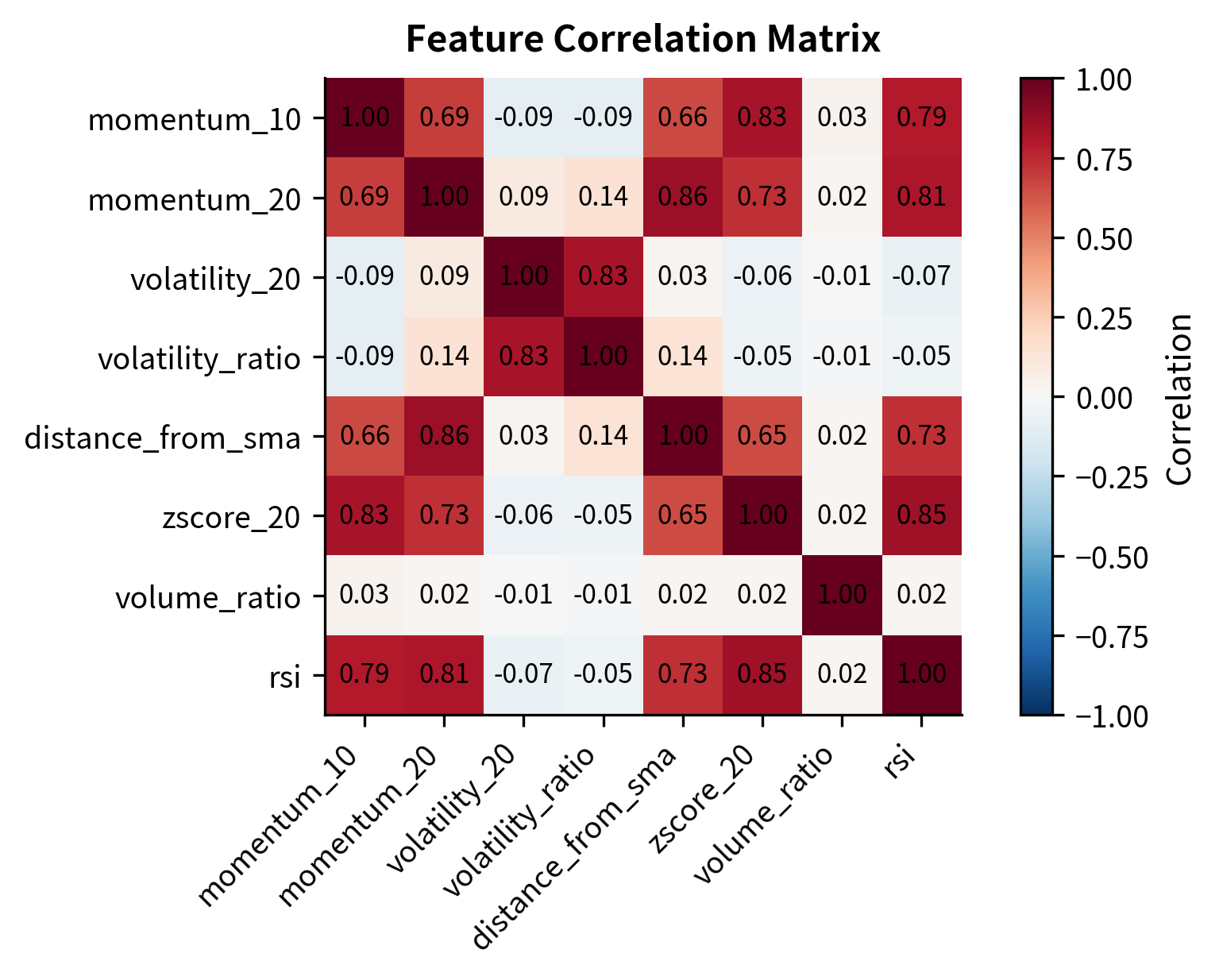
Correlation analysis identifies redundant features that provide overlapping information:
The correlation matrix reveals strong relationships between momentum indicators and between volatility measures. High correlation (multicollinearity) implies redundancy, suggesting that the model might not need all these features to capture the underlying signal.
Model-based feature importance provides another perspective, revealing which features contribute most to predictions:
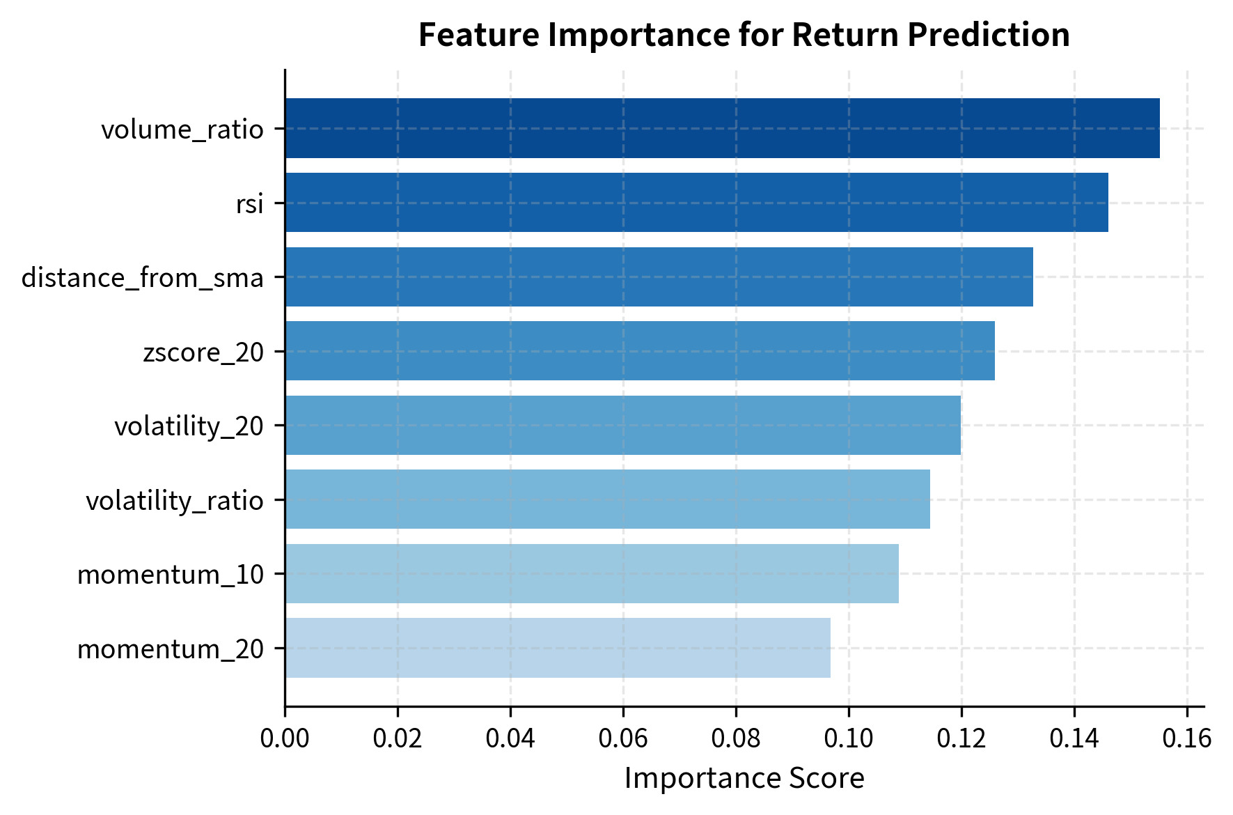
The feature importance rankings guide feature selection, but should be interpreted cautiously. Importance measures can be unstable, especially when features are correlated. Cross-validation of feature selection choices helps ensure robustness.
Model Validation and Overfitting Prevention
The fundamental challenge in machine learning for trading is overfitting: building models that perfectly capture patterns in historical data but fail to generalize to future, unseen data. Financial data presents particularly severe overfitting risks due to low signal-to-noise ratios, non-stationarity, and the temptation to test many hypotheses until something appears to work.
The Train-Test Split
The first line of defense against overfitting is evaluating model performance on data not used during training. A simple train-test split reserves a portion of the data (typically 20-30%) for evaluation. The reasoning is straightforward: if we evaluate on the same data used for training, the model can achieve artificially high performance by memorizing noise. By holding out data the model has never seen, we obtain an honest estimate of generalization performance.
However, for time series data like financial returns, a random split would allow future information to leak into training. Consider what happens if we randomly shuffle and split: some training observations might come from 2023 while some test observations come from 2020. The model could learn patterns from the future and apply them to the past, creating an impossibly favorable evaluation scenario that would never occur in practice.
Instead, we use a temporal split where training data precedes test data:
This sequential split mimics a real-world scenario where we train on history to predict the future. The training set allows the model to learn patterns, while the test set serves as a proxy for unseen future data. This approach respects the causal structure of time: we only use past information to predict future outcomes.
Time Series Cross-Validation
A single train-test split provides only one estimate of out-of-sample performance. Time series cross-validation generates multiple estimates by repeatedly training on expanding or sliding windows of historical data and testing on subsequent periods. This approach gives us a distribution of performance estimates, allowing us to assess not just average performance but also variability across different time periods.
The walk-forward validation approach mimics how models would actually be deployed: train on all available data up to time , predict for time , then retrain with data up to , predict for , and so on.
The variation across folds reveals how stable the model's performance is across different time periods. Large variation suggests the model may be sensitive to market regime changes, a warning sign for deployment.
Visualizing Walk-Forward Validation
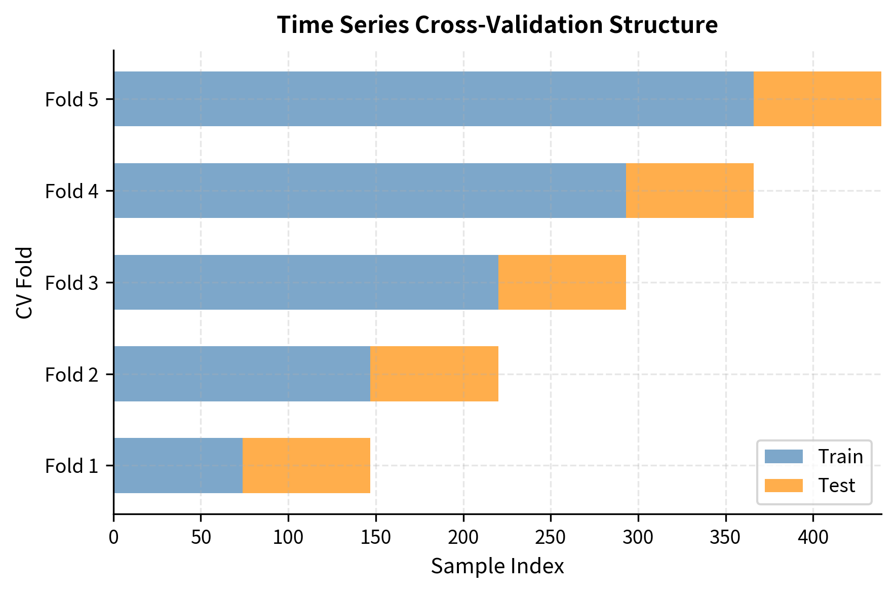
The plot confirms that the training window (blue) always precedes the test window (orange). This strict temporal separation ensures the model predicts future events using only past information, eliminating look-ahead bias.
Regularization Techniques
Regularization directly penalizes model complexity, preventing the model from fitting noise in the training data. The fundamental insight is that complex models with many large coefficients can fit training data perfectly but will perform poorly on new data. By adding a penalty term that grows with coefficient magnitude, we encourage the model to find simpler solutions that capture only the strongest patterns.
For linear models, L1 (Lasso) and L2 (Ridge) regularization add penalty terms to the loss function. These approaches represent different philosophies about what "simplicity" means.
Ridge regression minimizes:
where:
- : total loss function to be minimized
- : sum of squared errors (measures data fit)
- : L2 penalty term that shrinks coefficients toward zero
- : number of samples
- : number of features
- : actual value for sample
- : predicted value for sample
- : regularization strength parameter
- : coefficient for feature
The Ridge penalty, which squares each coefficient, penalizes large coefficients heavily but never forces them to exactly zero. This approach works well when we believe all features contribute some signal, just with varying importance. The penalty smoothly shrinks coefficients, with larger coefficients receiving proportionally larger penalties.
Lasso regression minimizes:
where:
- : total loss function to be minimized
- : sum of squared errors
- : L1 penalty term that can force coefficients to exactly zero
- : number of samples
- : number of features
- : actual value for sample
- : predicted value for sample
- : regularization strength parameter
- : coefficient for feature
The Lasso penalty, which uses absolute values rather than squares, has a remarkable property: it can force coefficients to exactly zero. This happens because the absolute value function has a sharp corner at zero, creating a mathematical incentive for coefficients to snap to zero rather than merely approach it. This behavior makes Lasso effective for automatic feature selection.
The hyperparameter controls the strength of regularization. L1 regularization tends to produce sparse models (many coefficients exactly zero), effectively performing feature selection. L2 regularization shrinks coefficients toward zero but rarely makes them exactly zero.
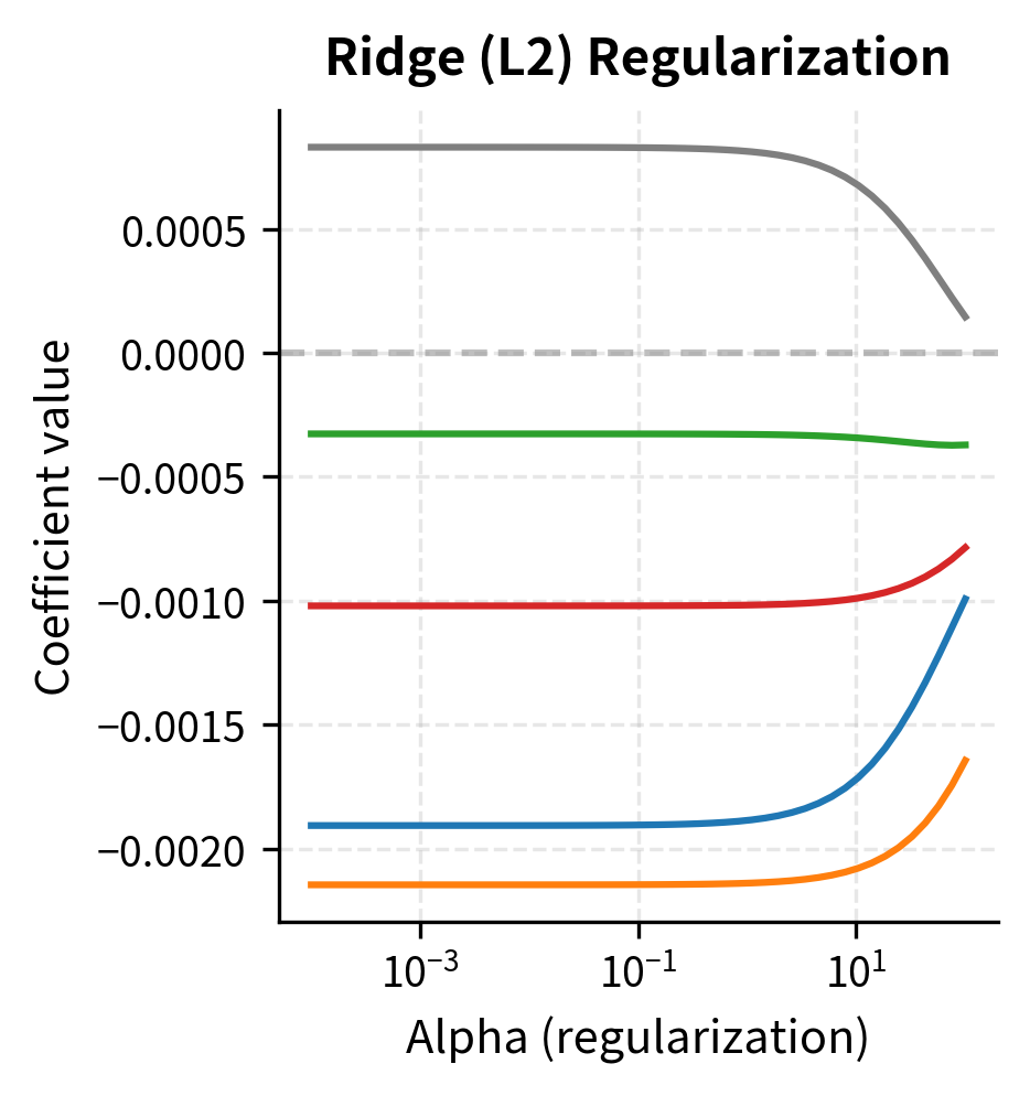
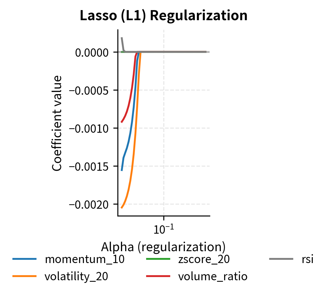
The results illustrate how increasing alpha reduces model complexity. As regularization strength grows, the number of non-zero coefficients in the Lasso model decreases, effectively selecting the most important features. While predictive accuracy (R²) dips slightly with very high regularization, the resulting models are often more robust to noise.
Key Parameters
The key parameters for regularized regression are:
- alpha: Constant that multiplies the penalty terms. Higher values imply stronger regularization.
- max_iter: The maximum number of iterations for the solver.
For tree-based methods, regularization takes different forms: limiting tree depth, requiring minimum samples per leaf, or constraining the number of features considered at each split. These constraints prevent trees from growing too deep and memorizing training data.
Model Evaluation Metrics
Choosing appropriate evaluation metrics is critical for assessing whether a model will be useful in practice. The right metric depends on the prediction task and how the model will be used in trading decisions.
Regression Metrics
For continuous predictions like return forecasts, common metrics include:
Mean Squared Error (MSE) measures the average squared difference between predictions and actual values:
where:
- : total number of samples
- : actual value for observation
- : predicted value for observation
MSE penalizes large errors heavily due to squaring, which may be appropriate when large prediction errors are particularly costly. In trading contexts, a model that occasionally makes huge errors might be more dangerous than one that makes consistent small errors, making MSE a sensible choice when tail risk matters.
Mean Absolute Error (MAE) provides a more robust measure, less sensitive to outliers:
where:
- : total number of samples
- : actual value
- : predicted value
Because MAE treats all errors linearly regardless of magnitude, it provides a more interpretable measure: the average MAE tells you the typical size of your prediction errors in the same units as your target variable.
R-squared () measures the proportion of variance explained by the model:
where:
- : residual sum of squares (unexplained variance)
- : total sum of squares (total variance)
- : actual value for sample
- : predicted value for sample
- : mean of the actual values
- : number of samples
This metric compares the model's errors to the variance of the target variable. An of 1 means the model perfectly predicts every observation; an of 0 means the model is no better than simply predicting the mean. Negative values indicate the model performs worse than this naive baseline.
In financial return prediction, values are typically very low (often below 0.05) because returns are inherently noisy. A seemingly tiny of 0.01 might still be valuable if it represents genuine predictive power.
Classification Metrics
For binary classification (predicting return direction, default events, etc.), metrics go beyond simple accuracy:
Accuracy measures the proportion of correct predictions:
where:
- : true positives (correctly predicted positive cases)
- : true negatives (correctly predicted negative cases)
- : false positives (incorrectly predicted positive cases)
- : false negatives (incorrectly predicted negative cases)
However, accuracy can be misleading with imbalanced classes. If positive returns occur 55% of the time, always predicting "positive" achieves 55% accuracy without any skill.
Precision and Recall focus on positive class predictions:
where:
- : true positives
- : false positives
where:
- : true positives
- : false negatives
Precision answers "of the times we predicted positive, how often were we right?" Recall answers "of all actual positives, how many did we catch?" These metrics often trade off against each other: being more selective (higher threshold) improves precision but reduces recall, and vice versa.
F1 Score balances precision and recall:
where:
- : proportion of positive predictions that were correct
- : proportion of actual positives that were correctly identified
The F1 score is the harmonic mean of precision and recall, which penalizes extreme imbalances between the two. A model with perfect precision but terrible recall (or vice versa) will have a mediocre F1 score, while balanced performance yields higher scores.
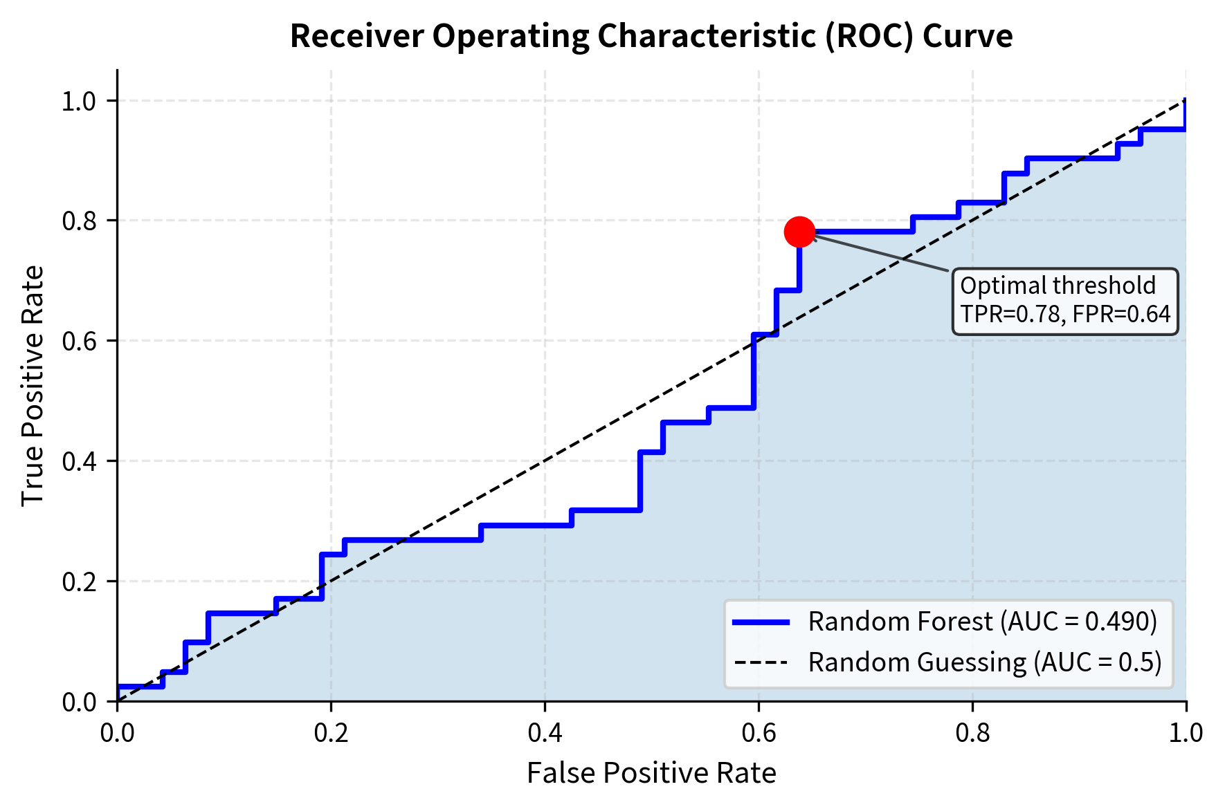
ROC-AUC (Area Under the Receiver Operating Characteristic Curve) measures discrimination ability across all classification thresholds, providing a threshold-independent assessment of model quality.
The accuracy of roughly 54% is typical for daily return prediction, where edges are small. However, the precision and recall balance (F1 Score) and the ROC-AUC above 0.50 confirm that the model contains genuine signal and outperforms random guessing.
Financial-Specific Metrics
Standard ML metrics don't directly measure what matters most in trading: profitability. Consider supplementing with finance-specific measures:
Directional Accuracy Improvement compares the model's directional accuracy to a naive baseline (random guessing or always predicting the majority class).
Profit Factor measures the ratio of gross profits to gross losses when using the model's predictions for trading decisions.
Information Coefficient (IC) measures the correlation between predicted and actual returns, which directly relates to potential alpha generation.
A profit factor above 1.0 indicates a profitable strategy, though practical trading would also account for transaction costs. The Sharpe ratio provides a risk-adjusted view; an annualized value around 1.0 or higher is typically targeted by quantitative funds.
Pitfalls and Best Practices
Machine learning offers powerful tools for pattern recognition, but applying these tools to financial markets requires navigating a minefield of potential errors. Understanding these pitfalls is as important as understanding the algorithms themselves.
Overfitting to Historical Data
The most pervasive danger in quantitative finance is overfitting: discovering patterns that exist only in historical data due to random chance. With enough feature combinations and model configurations, you can almost always find something that worked in the past. The problem is that random patterns don't persist.
The low signal-to-noise ratio in financial returns amplifies this problem. When predicting equity returns with even modest noise levels, spurious patterns that explain in-sample variation can easily masquerade as genuine predictive signals. A model achieving 60% in-sample accuracy might be capturing 55% real signal and 5% noise, with no way to distinguish between them until out-of-sample testing. Multiple testing compounds the issue. If you test 100 strategies and keep the one with the best backtest, you've implicitly optimized for in-sample performance even if each strategy seemed reasonable a priori. The solution is to reserve truly untouched test data for final evaluation, and to apply statistical corrections (like the Bonferroni correction or false discovery rate control) when testing multiple hypotheses.
Non-Stationarity of Markets
Financial markets evolve continuously. Relationships that existed in the past may weaken, disappear, or reverse as market participants adapt. The statistical properties of returns themselves shift across market regimes (bull markets, bear markets, high-volatility periods, low-volatility periods).
A structural shift in market dynamics, such as a change in volatility levels, correlation patterns, or the effectiveness of certain trading strategies. Models trained on one regime may perform poorly when the regime changes.
This non-stationarity means that even a model that generalizes well to held-out test data from the same historical period may fail when deployed in live trading. Regular model retraining with recent data helps, but doesn't eliminate the fundamental challenge that the future may be unlike the past in ways we cannot anticipate.
Look-Ahead Bias
Look-ahead bias occurs when information that wouldn't have been available at the time of a trading decision inadvertently enters the model. Common sources include:
- Using revised economic data instead of the originally reported values
- Computing features using the full time series (e.g., standardizing with full-sample mean and standard deviation)
- Aligning events with prices incorrectly (e.g., using closing prices for events that occurred after market close)
Even subtle forms of look-ahead bias can dramatically inflate backtested performance. Feature engineering must carefully respect the temporal flow of information, using only data that would have been available at each prediction point.
The Need for Interpretability
Black-box models that achieve slightly better predictive accuracy may be less valuable than simpler models whose behavior is understandable. Interpretability matters for several reasons:
- Debugging: When a model performs poorly, interpretable models allow diagnosis of what went wrong
- Adaptation: Understanding why a model works helps predict when it might stop working
- Risk Management: Unexplainable models create operational and regulatory risks
- Confidence: Traders and portfolio managers are more likely to follow signals they understand
Techniques like SHAP (SHapley Additive exPlanations) values and partial dependence plots can provide post-hoc interpretability for complex models, but starting with inherently interpretable models (linear models, shallow decision trees) often proves more practical.
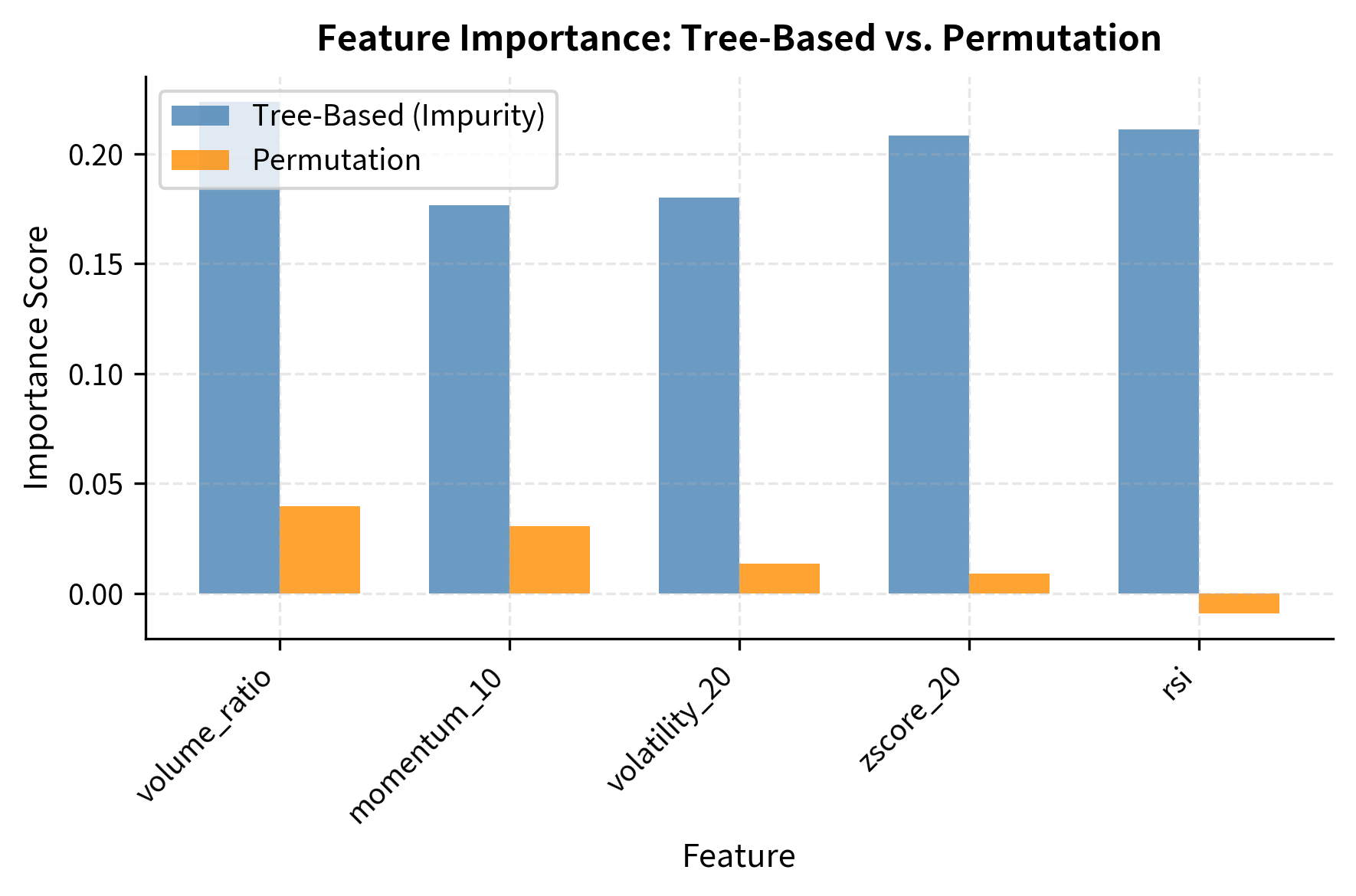
Permutation importance often provides a more reliable ranking than impurity-based importance (Tree-Based), which can be biased toward high-cardinality features. Discrepancies between the two methods suggest we should investigate those features further before relying on them.
Best Practices Summary
Given these pitfalls, the following practices help build more robust trading models:
- Use time-aware validation: Always split data temporally and use walk-forward cross-validation
- Start simple: Begin with interpretable models like linear regression or shallow trees before trying complex methods
- Engineer features thoughtfully: Draw on domain knowledge from established trading strategies rather than blindly generating hundreds of features
- Regularize aggressively: When in doubt, prefer simpler models with more regularization
- Validate on truly held-out data: Reserve a final test set that's never used for model selection or hyperparameter tuning
- Monitor in production: Track live performance against expectations and investigate discrepancies promptly
- Accept modest performance: In finance, small edges compound over time. A model with 52% directional accuracy might be valuable; one claiming 70% accuracy is probably overfit
Complete Worked Example
Let's bring together the concepts from this chapter in a complete example that demonstrates the full workflow from data preparation through model evaluation.
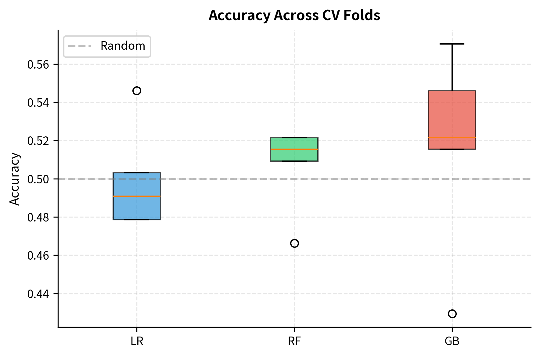
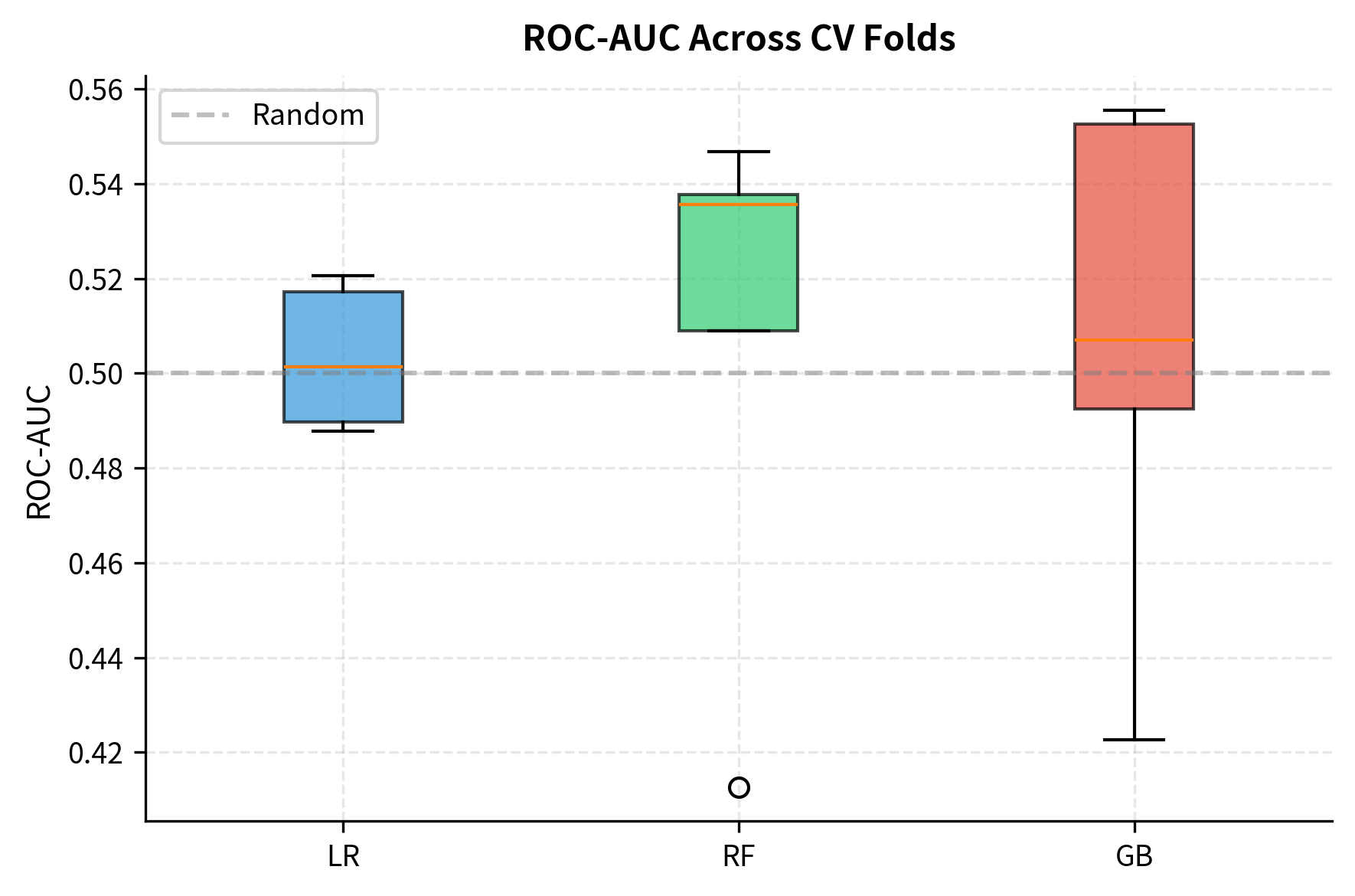
The cross-validation results show modest but consistent predictive ability across all three models, with accuracies slightly above 50% and ROC-AUC values above 0.5. This is realistic for financial return prediction: even small edges can be valuable when applied systematically over time.
Summary
Machine learning provides powerful tools for discovering patterns in financial data, but successful application requires understanding both the algorithms and the unique challenges of financial prediction.
We covered the main categories of machine learning, including supervised, unsupervised, and reinforcement learning, with emphasis on supervised methods most commonly used in trading. Linear models provide interpretability and serve as baselines, while tree-based ensembles (random forests and gradient boosting) often achieve superior performance on tabular financial data. Neural networks offer even greater flexibility but require more data and careful tuning.
Feature engineering transforms raw market data into informative model inputs. Drawing on domain knowledge from established trading strategies (momentum indicators, mean reversion signals, volatility measures) typically outperforms naive feature generation. Feature selection and importance analysis help identify which features contribute genuine predictive power.
Rigorous validation is essential for avoiding overfitting. Time series cross-validation with walk-forward procedures mimics real deployment conditions, while regularization directly penalizes model complexity. Evaluation metrics should align with trading objectives; beyond standard ML metrics like accuracy and AUC, consider financial measures like Sharpe ratio and profit factor.
Finally, we discussed the major pitfalls in applying ML to trading: overfitting to historical patterns, non-stationarity of markets, look-ahead bias, and the trade-off between model complexity and interpretability. Awareness of these challenges, combined with disciplined validation practices, helps build models that generalize to live trading rather than merely fitting historical noise.
The next chapter builds on these foundations by exploring how to integrate machine learning into complete trading strategy design, including combining ML predictions with traditional quantitative methods and managing the practical challenges of model deployment.
Quiz
Ready to test your understanding? Take this quick quiz to reinforce what you've learned about machine learning techniques for trading.

Comments