

A comprehensive guide to XGBoost (eXtreme Gradient Boosting), including second-order Taylor expansion, regularization techniques, split gain optimization, ranking loss functions, and practical implementation with classification, regression, and learning-to-rank examples.

This article is part of the free-to-read Machine Learning from Scratch
Choose your expertise level to adjust how many terms are explained. Beginners see more tooltips, experts see fewer to maintain reading flow. Hover over underlined terms for instant definitions.
XGBoost
XGBoost (eXtreme Gradient Boosting) represents a highly optimized implementation of gradient boosting that has become one of the most successful machine learning algorithms in practice. Building on the foundation of boosted trees that we've already explored, XGBoost introduces several key innovations that make it exceptionally fast, memory-efficient, and accurate. The algorithm was specifically designed to push the boundaries of what's possible with gradient boosting, incorporating advanced optimization techniques and engineering improvements that have made it a go-to choice for many machine learning competitions and production systems.
At its core, XGBoost follows the same fundamental principle as other gradient boosting methods: it builds an ensemble of weak learners (typically decision trees) sequentially, where each new tree corrects the errors made by the previous ones. However, what sets XGBoost apart is its sophisticated approach to optimization, including second-order gradient information, advanced regularization techniques, and highly efficient computational implementations. These innovations allow XGBoost to achieve superior performance while being more computationally efficient than traditional gradient boosting implementations.
The algorithm's name reflects its focus on "extreme" optimization—it was designed to be one of the fastest and most accurate gradient boosting implementations available. This optimization extends beyond just the mathematical formulation to include careful attention to system-level performance, memory usage, and parallelization strategies. As a result, XGBoost has become particularly popular in scenarios where both accuracy and computational efficiency are critical, such as large-scale machine learning competitions, real-time prediction systems, and applications requiring rapid model training and deployment.
Advantages
XGBoost offers several compelling advantages that have contributed to its widespread adoption. First and foremost, it provides exceptional predictive performance across a wide variety of machine learning tasks, consistently ranking among the top performers in machine learning competitions and benchmarks. This superior accuracy stems from its sophisticated regularization techniques, including both L1 (Lasso) and L2 (Ridge) regularization on the tree structure and leaf weights, which helps prevent overfitting while maintaining model complexity.
The algorithm's computational efficiency represents another major advantage. XGBoost implements several optimization techniques that make it significantly faster than traditional gradient boosting implementations, including parallel processing capabilities, cache-aware data structures, and optimized memory usage patterns. These improvements allow practitioners to train complex models on large datasets in reasonable time frames, making XGBoost practical for real-world applications where computational resources are limited.
XGBoost also provides excellent flexibility and ease of use. The algorithm can handle various types of data (numerical, categorical, text) without extensive preprocessing, includes built-in cross-validation capabilities, and offers comprehensive hyperparameter tuning options. Additionally, it provides detailed feature importance measures and model interpretability tools, making it valuable not just for prediction but also for understanding the underlying patterns in the data.
Disadvantages
Despite its many strengths, XGBoost does have some limitations that practitioners should consider. The algorithm can be computationally intensive, particularly when dealing with very large datasets or when using many boosting rounds. While XGBoost is more efficient than traditional gradient boosting, it can still require significant computational resources for optimal performance, especially when extensive hyperparameter tuning is needed.
XGBoost's complexity can also be a disadvantage in certain scenarios. The algorithm has many hyperparameters that can be tuned, which can make it challenging to optimize without proper understanding of their effects. This complexity can lead to overfitting if not managed carefully, and the extensive tuning process can be time-consuming and computationally expensive. Additionally, while XGBoost provides some interpretability features, the resulting models are still ensemble methods that can be more difficult to interpret than simpler algorithms like linear regression or single decision trees.
Another consideration is that XGBoost, like other tree-based methods, can struggle with certain types of data relationships. It may not perform as well on data with strong linear relationships where simpler methods might be more appropriate, and it can be sensitive to outliers in the training data. Additionally, while XGBoost can handle missing values, the approach may not be optimal for datasets with extensive missing data patterns.
Formula
The mathematical foundation of XGBoost is rooted in the general gradient boosting framework, but XGBoost introduces several crucial innovations that make it both more powerful and more efficient. To understand how XGBoost works under the hood, let's break down its formulation step by step, carefully explaining the meaning and purpose of each component.
1. The Objective Function
At each boosting iteration , XGBoost seeks to minimize an objective function that balances two goals:
- Fitting the data well (minimizing prediction error)
- Controlling model complexity (to avoid overfitting)
The general form of the objective function at iteration is:
- is the number of training examples.
- is a differentiable loss function (e.g., squared error for regression, log-loss for classification).
- is the true label for instance .
- is the prediction for after trees (i.e., the current ensemble's output).
- is the output of the new tree being added at iteration .
- is a regularization term that penalizes the complexity of the new tree.
At each step, XGBoost adds a new tree to the ensemble, aiming to improve predictions while keeping the model as simple as possible.
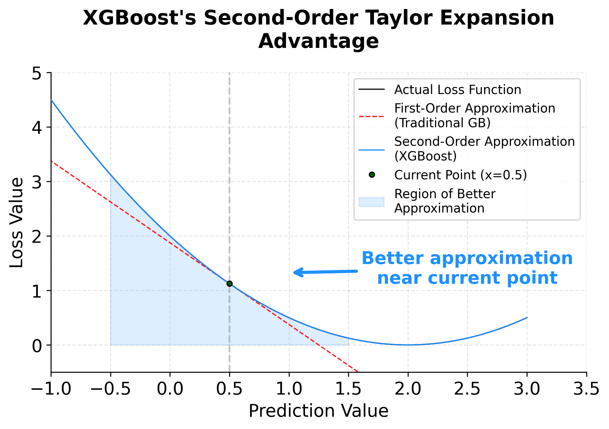
2. Second-Order Taylor Expansion
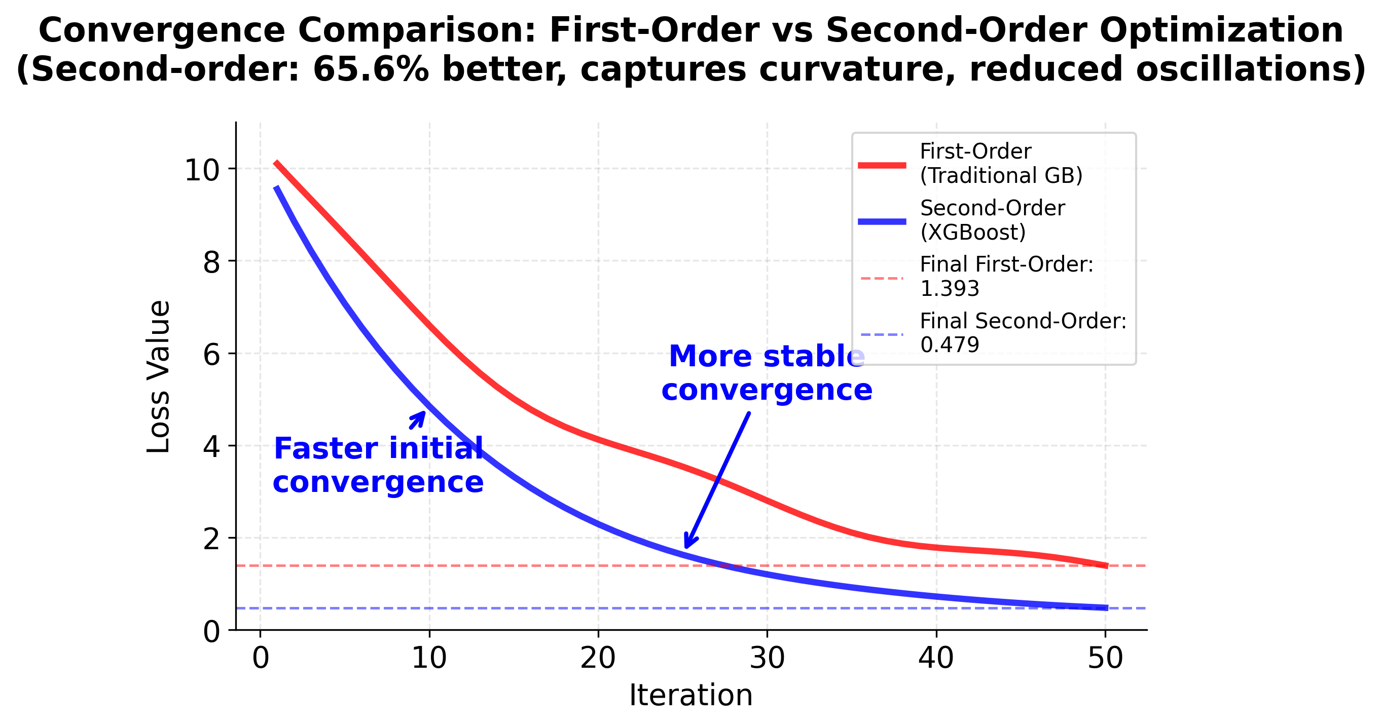
A key innovation in XGBoost is the use of a second-order Taylor expansion to approximate the loss function. This allows XGBoost to use both the gradient (first derivative) and the curvature (second derivative, or Hessian) of the loss, leading to more accurate and stable optimization compared to traditional gradient boosting, which uses only the first derivative.
Note: The second-order Taylor expansion is a mathematical technique that approximates a function near a point using both its slope (first derivative) and curvature (second derivative). This provides a more accurate approximation than using only the slope, especially when the function has significant curvature. In XGBoost, this translates to better optimization steps and faster convergence.
For each data point , we expand the loss function around the current prediction :
where:
- is the first-order gradient (how much the loss would change with a small change in prediction).
- is the second-order gradient (how the gradient itself changes; i.e., the curvature).
This is important because:
- The first-order term () tells us the direction to move to reduce the loss.
- The second-order term () tells us how confident we are in that direction (steepness/curvature).
- Using both allows for more precise and robust updates, especially for complex loss functions.
To understand why second-order information is valuable, consider how gradient and Hessian guide optimization differently:
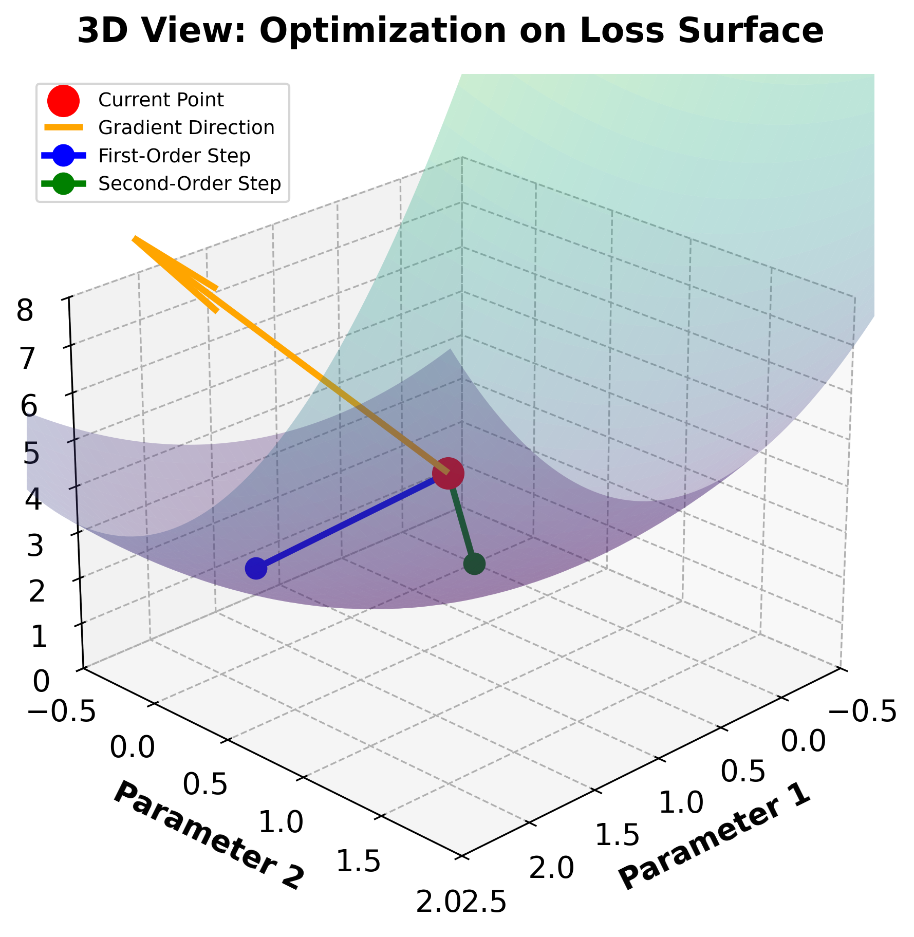
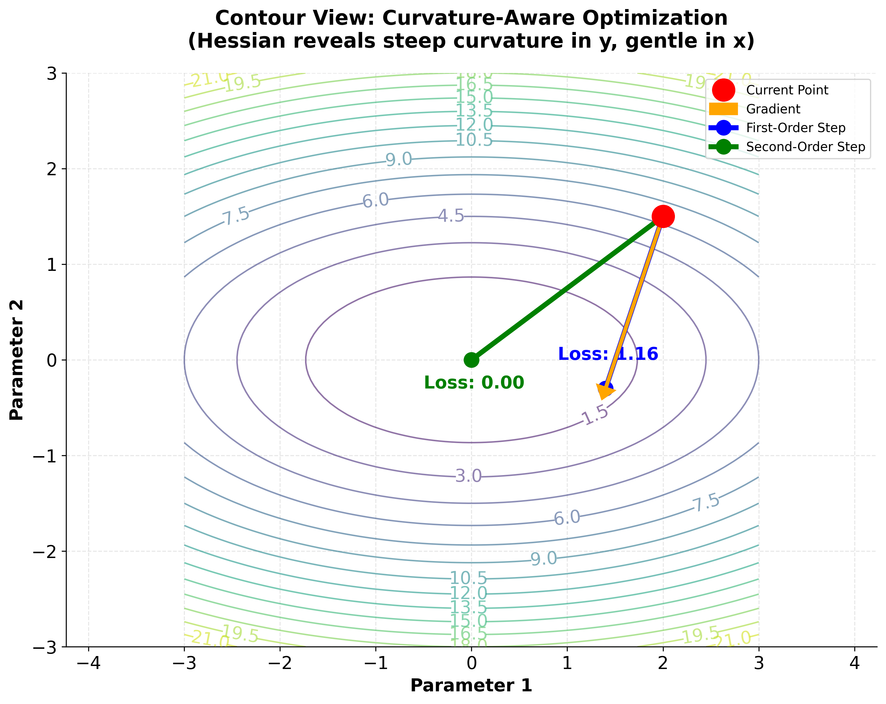
The visualization demonstrates a key advantage of using second-order information: the Hessian allows XGBoost to adapt step sizes based on local curvature. In the contour plot, notice how the loss surface has different curvature in different directions (the elliptical contours). The first-order method (blue) uses a fixed step size and overshoots in the steep direction, while the second-order method (green) uses curvature information to take a more appropriate step, achieving a lower loss value. This curvature-aware optimization is why XGBoost converges faster and more reliably than traditional gradient boosting.
3. Approximated Objective Function
Plugging the Taylor expansion into the original objective, and noting that is constant with respect to , we get:
- The sum over encourages the new tree to correct the errors of the current model.
- The sum over penalizes large updates, especially where the loss curve is steep (high curvature).
4. Regularization Term
XGBoost's regularization term is more sophisticated than in standard boosting. It penalizes both the complexity of the tree structure and the magnitude of the leaf weights:
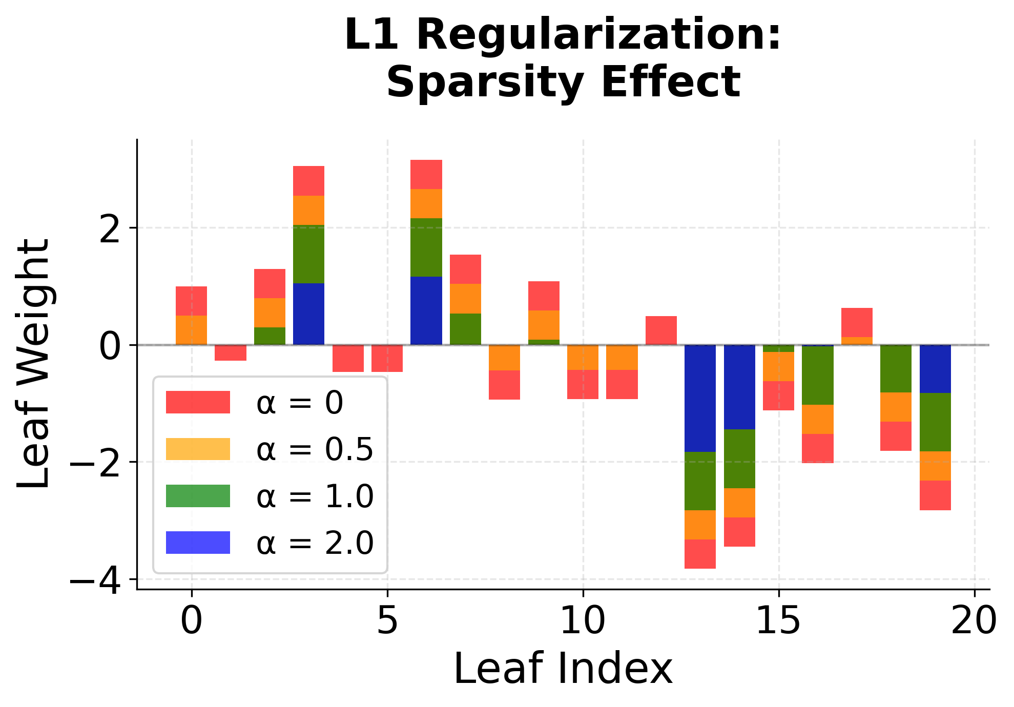
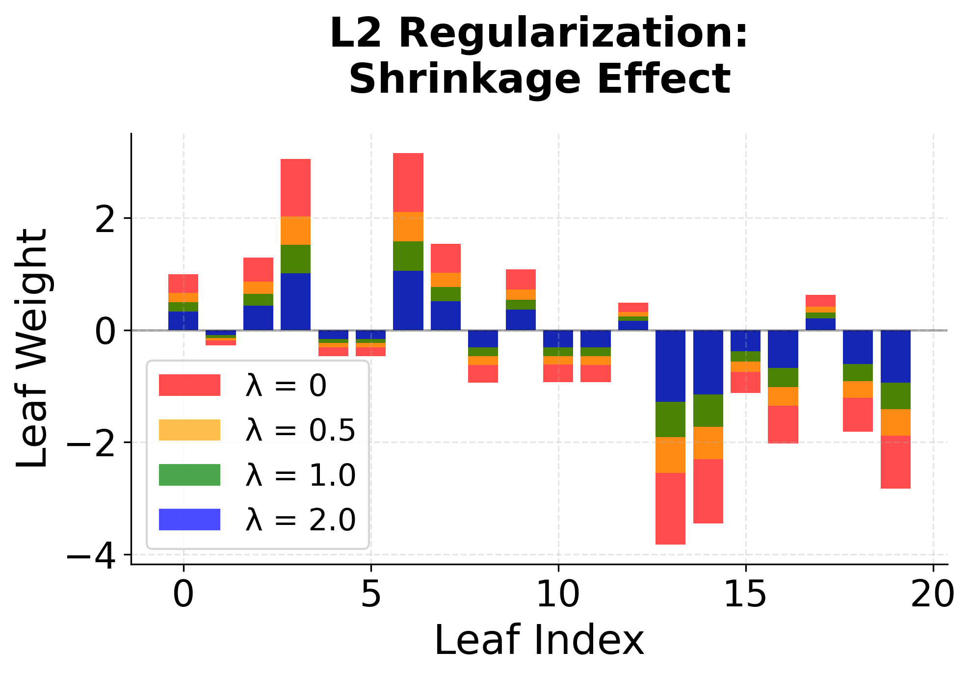
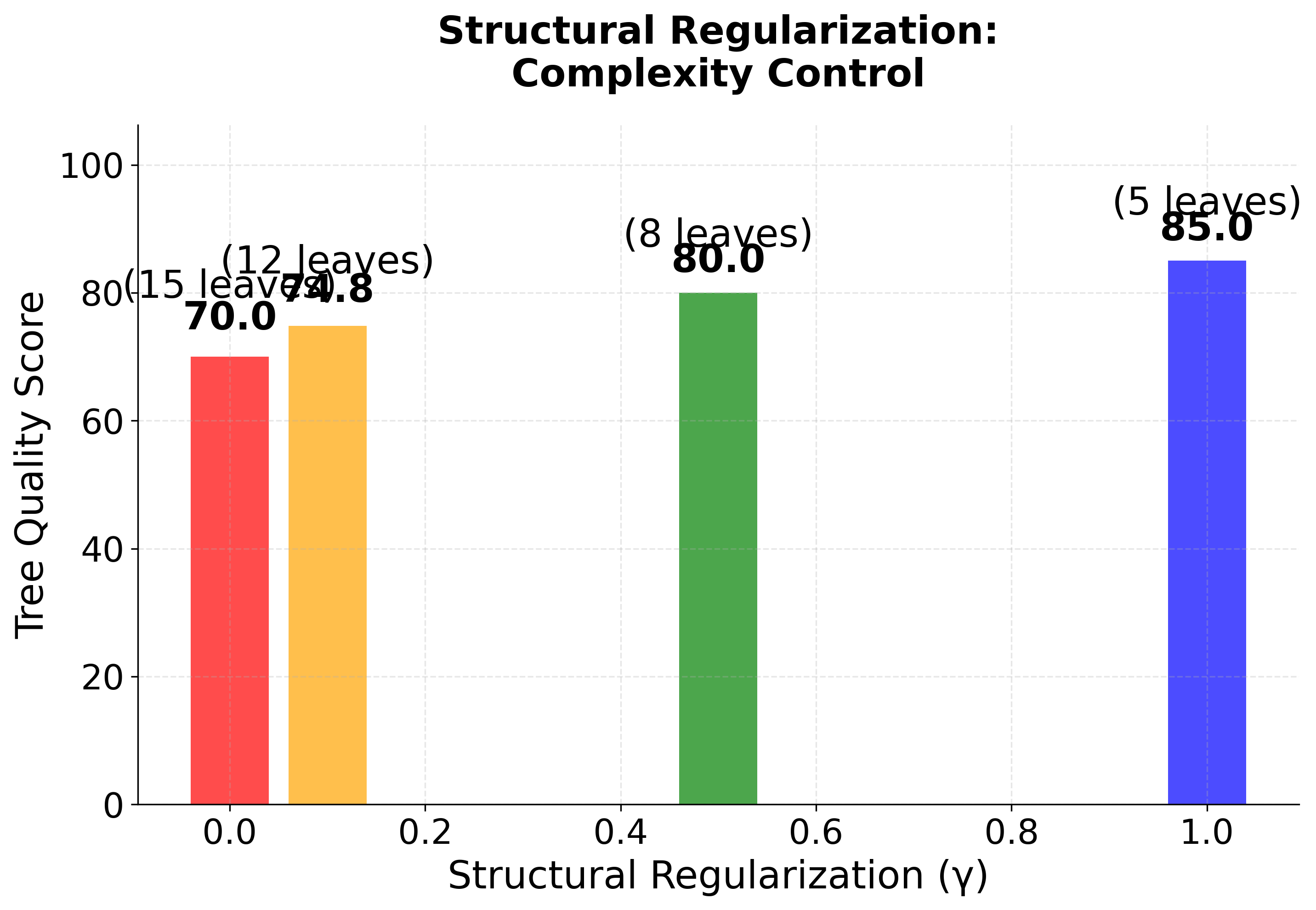
Note: Regularization in XGBoost serves multiple purposes: it prevents overfitting by controlling model complexity, encourages sparsity in leaf weights (L1), and provides smooth shrinkage (L2). The structural regularization () specifically controls tree complexity by penalizing the number of leaves, encouraging simpler trees that generalize better.
- is the number of leaves in the tree .
- is the score (weight) assigned to leaf .
- penalizes having too many leaves (encourages simpler trees).
- is the L2 regularization parameter (shrinks large leaf weights).
- is the L1 regularization parameter (encourages sparsity in leaf weights).
This regularization helps prevent overfitting by discouraging overly complex trees and large leaf values.
5. Rewriting the Objective in Terms of Leaves
Let's break down how the objective function is rewritten in terms of the leaves of a tree, step by step.
Partitioning the Data by Leaves
When we build a decision tree, each data point ends up in exactly one leaf. Suppose the tree has leaves. For each leaf (where ), define:
- : the set of indices of data points that fall into leaf . Here, is a function that tells us which leaf belongs to.
- : the score or weight assigned to leaf . Every data point in leaf gets the same output from the tree.
Expanding the Objective Function
Let's expand in detail how the objective function is rewritten in terms of the leaves of the tree.
Recall the approximated objective function after the second-order Taylor expansion:
where:
- is the first derivative (gradient) of the loss with respect to the prediction for ,
- is the second derivative (Hessian) of the loss with respect to the prediction for ,
- is the output of the new tree for ,
- is the regularization term for the tree.
Grouping by Leaves
A decision tree partitions the data into leaves. Each data point falls into exactly one leaf, say leaf . Let:
- be the set of indices of data points assigned to leaf ,
- be the score (weight) assigned to leaf .
By the definition of a tree, for all , the output of the tree is the same:
- for all .
This allows us to rewrite the sums over all data points as sums over leaves, grouping together all points in the same leaf.
Expanding the First-Order Term (Step-by-Step)
Let's break down how to rewrite the first-order term by grouping data points according to the leaves they fall into:
-
Start with the original first-order term:
-
Group data points by their assigned leaf:
Each data point is assigned to a leaf , so we can rewrite the sum over all data points as a sum over leaves and, within each leaf, a sum over the data points in that leaf: -
Substitute the leaf weight for the tree output:
For all in leaf , , so we can replace with : -
Factor out terms that do not depend on :
is constant for all in , so we can factor it out of the inner sum: -
Write the final grouped form:
This shows that the first-order term for the whole tree is the sum, over all leaves, of the sum of gradients in each leaf times the leaf's weight:
This step-by-step grouping is important because it allows us to efficiently compute the contribution of each leaf to the objective function.
Expanding the Second-Order Term
Let's break down how to rewrite the second-order term by grouping data points according to the leaves they fall into:
-
Start with the original second-order term:
-
Group data points by their assigned leaf:
Each data point is assigned to a leaf , so we can rewrite the sum over all data points as a sum over leaves and, within each leaf, a sum over the data points in that leaf: -
Substitute the leaf weight for the tree output:
For all in leaf , , so we can replace with : -
Factor out terms that do not depend on :
is constant for all in , so we can factor it out of the inner sum: -
Write the final grouped form:
This shows that the second-order term for the whole tree is the sum, over all leaves, of the sum of Hessians in each leaf times the square of the leaf's weight (with a factor of ):
This step-by-step grouping is important because it allows us to efficiently compute the contribution of each leaf to the objective function.
Putting It Together
So, the original sum over all data points can be rewritten as a sum over leaves, where each leaf's contribution depends on the sum of gradients and Hessians of the data points it contains, and the leaf's weight:
This grouping is crucial because it allows XGBoost to efficiently compute the optimal weights for each leaf and to evaluate the quality of different tree structures.
Adding Regularization
The regularization term for the tree is:
- penalizes the number of leaves (to discourage overly complex trees).
- and penalize large or non-sparse leaf weights.
Note: This is basically L1 and L2 regularization that we learned in the previous chapters but applied to the leaf weights.
Putting It All Together
Let's carefully combine the grouped sums from the objective and the regularization terms, step by step.
Recall from above that, after grouping by leaves, the second-order Taylor-approximated objective (before regularization) is:
Now, let's add the regularization term for the tree:
So, the total objective at step is:
Let's write all terms involving together, grouping by leaf :
Now, notice that the two quadratic terms in can be combined for each leaf :
So, the objective simplifies to:
Or, written out for clarity:
This is the final grouped and regularized form of the objective for a single boosting step in XGBoost.
What does this mean?
- For each leaf , we sum up all the gradients () and Hessians () of the data points that fall into that leaf.
- The objective for the whole tree is now just a sum over the leaves, where each leaf's contribution depends on its weight , the total gradient and Hessian in that leaf, and the regularization terms.
- This form makes it possible to analytically solve for the best for each leaf, and to efficiently evaluate how good a particular tree structure is.
By grouping the data by leaves, we turn a sum over all data points into a sum over leaves, where each leaf's effect on the objective depends only on the data points it contains. This is the key step that allows XGBoost to efficiently optimize tree structures and leaf values.
6. Finding the Optimal Leaf Weights
To determine the best value for each leaf weight , we take the derivative of the objective with respect to and set it to zero (for simplicity, let's ignore the L1 term for now):
Note: The L1 regularization term () is non-differentiable at zero, which complicates the analytical solution. In practice, XGBoost uses soft thresholding techniques to handle L1 regularization, but for this derivation, we focus on the L2 case to demonstrate the core mathematical principle.
Start with the grouped objective for a single leaf :
where
- (sum of gradients in leaf )
- (sum of Hessians in leaf )
Take the derivative with respect to :
Set the derivative to zero to find the minimum:
Solve for :
Substituting back the definitions:
- The optimal weight for each leaf is determined by the sum of gradients (how much the model is under- or over-predicting) and the sum of Hessians (how "confident" we are in those gradients), regularized by .
- This formula is used to assign the value to each leaf during tree construction.
To visualize how this optimization works, consider how the objective function for a single leaf varies with the leaf weight :
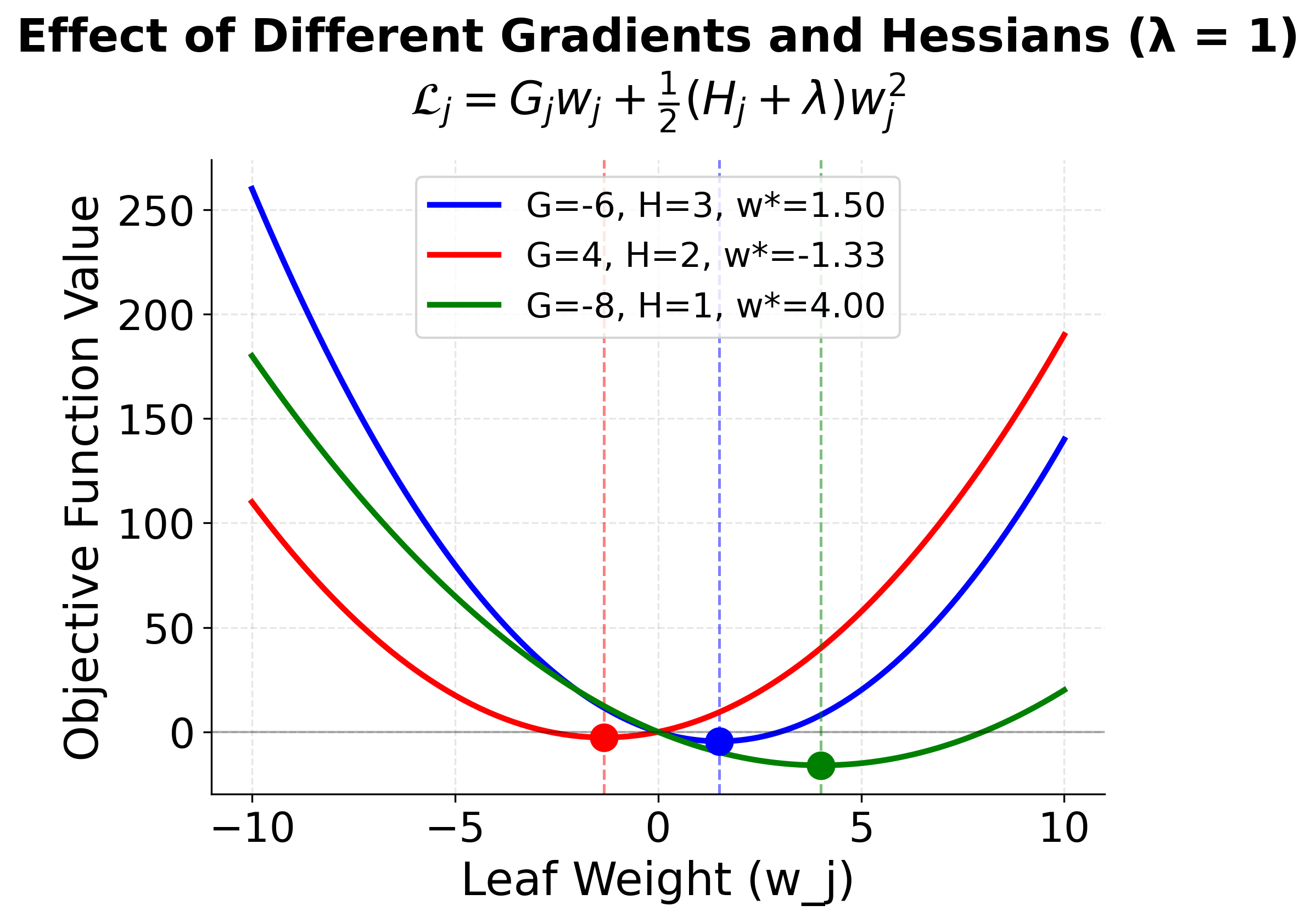
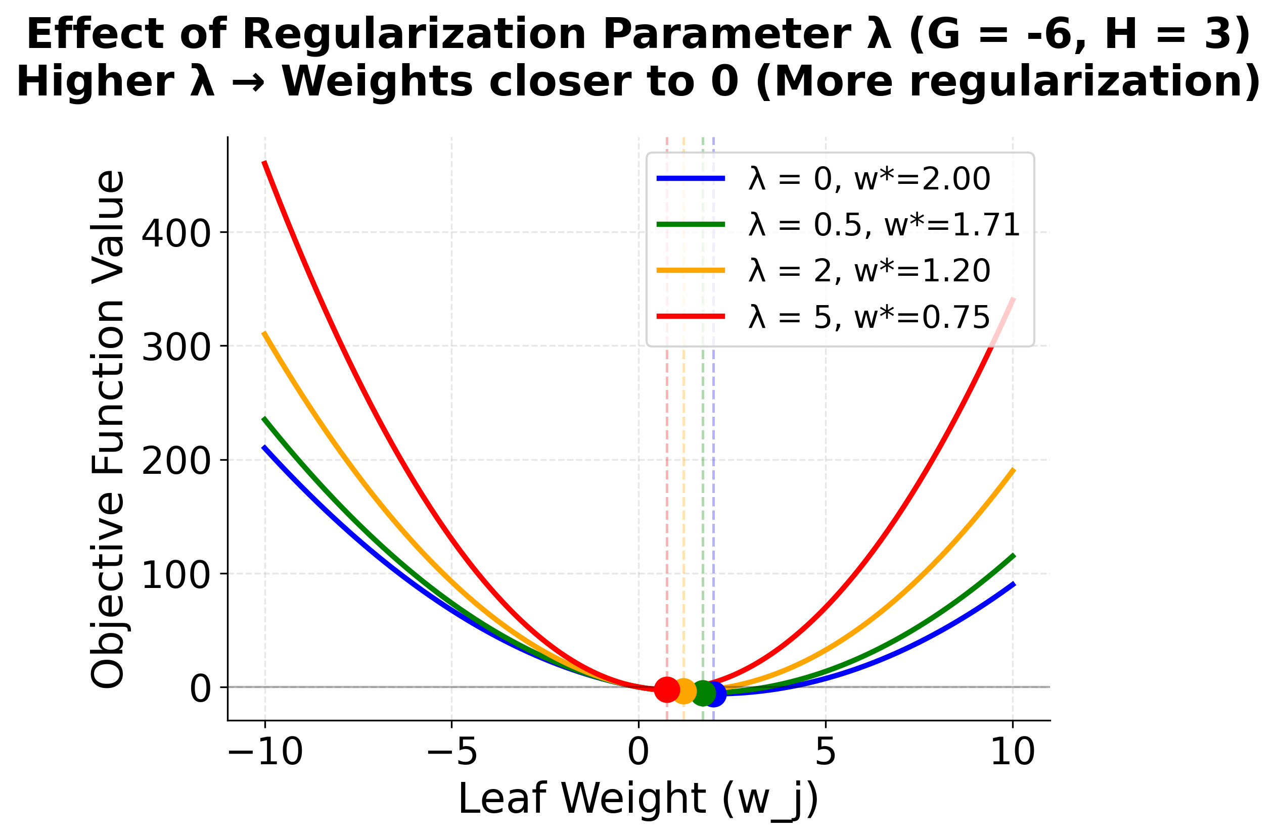
The visualization reveals how XGBoost finds optimal leaf weights through a simple quadratic optimization. The left plot shows how different gradient and Hessian values shift the location of the minimum—negative gradients push the optimum to positive weights (and vice versa), while larger Hessians create steeper curves that concentrate the optimum. The right plot demonstrates regularization's effect: as increases, the optimal weight is pulled toward zero, preventing overfitting by penalizing large leaf values. This analytical solution is one of XGBoost's key advantages—rather than iteratively searching for good weights, it can compute the exact optimum for each leaf given the tree structure.
7. The Structure Score (Split Gain)
When building the tree, XGBoost evaluates possible splits by computing the "gain" or "quality score" for a given tree structure. This is the improvement in the objective function if we use a particular split:
- The numerator rewards splits that group together data points with similar gradients (i.e., similar errors).
- The denominator penalizes splits where the model is less confident (low Hessian sum) or where regularization is strong.
- The term penalizes having too many leaves.
How is this used?
- During tree construction, XGBoost greedily chooses splits that maximize the reduction in this score (i.e., the largest gain).
- This process continues recursively, subject to constraints like maximum depth or minimum gain.
To understand how XGBoost evaluates and selects splits, consider a concrete example with multiple candidate splits:
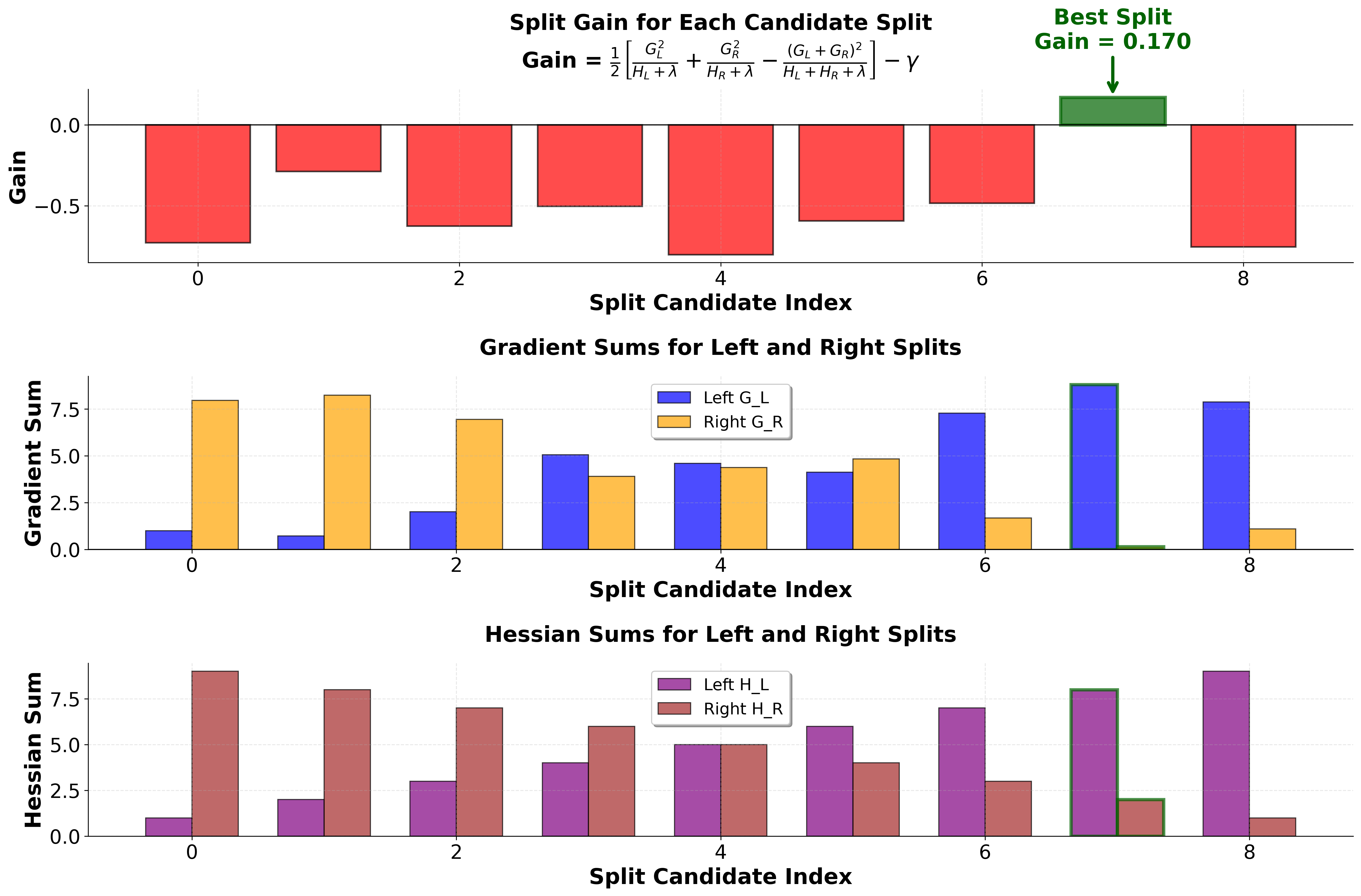
This visualization demonstrates XGBoost's greedy split selection process in action. The algorithm evaluates each possible split point by calculating how much the objective function would improve if that split were made. The gain formula balances three components: the quality of the left child (how well grouped its gradients are), the quality of the right child, and the cost of adding complexity (the penalty). Notice how some splits have negative gain—these would make the model worse and are rejected. The split with the highest positive gain (highlighted in dark green) is selected, and the process repeats recursively for each child node. This greedy approach, combined with the analytical gain formula, allows XGBoost to efficiently build effective tree structures without exhaustive search.
In summary, the structure score is used to guide the tree construction process:
- XGBoost's formula starts from the general gradient boosting objective, but uses a second-order Taylor expansion for more accurate optimization.
- It incorporates advanced regularization to control model complexity.
- The optimal leaf weights and split decisions are derived analytically using the gradients and Hessians of the loss function.
- This mathematical machinery enables XGBoost to build highly accurate, robust, and efficient tree ensembles.
Mathematical properties
The second-order approximation in XGBoost provides several important mathematical advantages. By incorporating the Hessian matrix (second derivatives), the algorithm can make more informed decisions about the direction and magnitude of updates, leading to faster convergence and better final performance. This is particularly beneficial when the loss function has significant curvature, as the second-order information captures this curvature more accurately than first-order methods alone.
Note: The mathematical presentation here focuses on the key concepts and simplified formulations. In practice, XGBoost's implementation includes additional optimizations such as approximate algorithms for split finding, handling of missing values, and various computational optimizations that are beyond the scope of this mathematical overview.
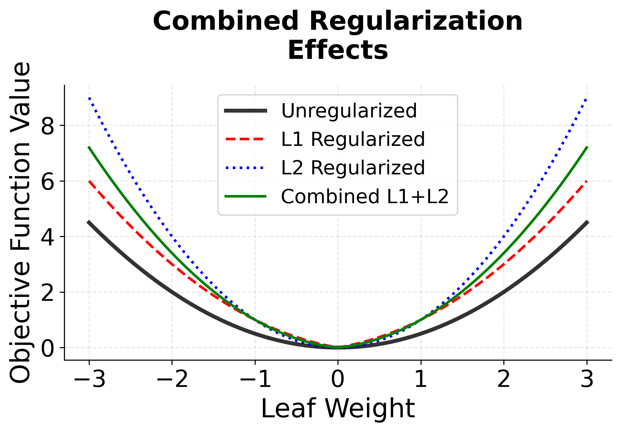
The regularization terms in XGBoost serve multiple purposes. The L2 regularization () helps prevent overfitting by penalizing large leaf weights, while the L1 regularization () can lead to sparsity in the leaf weights, effectively performing feature selection. The structural regularization () controls the complexity of the tree by penalizing the number of leaves, encouraging simpler trees that are less likely to overfit.
Ranking Loss Functions
Learning to rank is a type of machine learning problem where the goal is to automatically order or rank a set of items—such as documents, products, or recommendations—so that the most relevant items appear at the top of the list for a given query or context.
Unlike traditional regression or classification, which predict absolute values or categories, learning to rank focuses on optimizing the relative ordering of items based on their predicted relevance or usefulness. This approach is widely used in search engines, recommendation systems, and information retrieval, where presenting the most relevant results first is crucial for user satisfaction.
XGBoost supports various ranking loss functions that are essential for learning-to-rank applications. These loss functions are designed to optimize the relative ordering of items rather than their absolute scores.
Note: A deeper dive into the mathematical details and implementation of ranking loss functions will be provided in the classification section of this book.
Pairwise Ranking Loss
The pairwise ranking loss is designed to ensure that, for each query, the model learns to correctly order pairs of items according to their true relevance. The intuition is that, rather than predicting absolute scores, the model should focus on the relative ordering between items. For a query with items and , if item should be ranked higher than item (i.e., ), the model is penalized if it predicts otherwise.
Mathematically, the pairwise loss is:
where:
- is the set of all pairs such that item should be ranked above item for the same query.
- and are the predicted scores for items and .
Intuition:
- If (the model ranks much higher than ), the loss for that pair is close to zero.
- If (the model ranks below or equal to ), the loss is large, penalizing the model.
The loss is minimized when all relevant pairs are correctly ordered.
This approach is used in algorithms like RankNet and is the basis for XGBoost's "rank:pairwise" objective. It is especially effective when the main concern is the relative order of items, not their absolute scores.
Listwise Ranking Loss (NDCG)
The listwise ranking loss directly optimizes the quality of the entire ranked list, rather than focusing on individual pairs. One of the most popular listwise metrics is the Normalized Discounted Cumulative Gain (NDCG), which measures the usefulness, or gain, of an item based on its position in the result list, with higher gains for relevant items appearing earlier.
The NDCG for a single query is:
where:
- is the true relevance score of the item at position in the ranked list (with being the top position).
- is a normalization factor (the ideal DCG for that query), ensuring the score is between 0 and 1.
- The denominator discounts the gain for lower-ranked positions, reflecting that users pay more attention to top results.
The listwise loss is typically defined as the negative NDCG (since we want to maximize NDCG):
Intuition:
- The model is directly encouraged to produce rankings that maximize the overall usefulness of the list, especially at the top positions.
- Swapping two items with very different relevance scores near the top of the list will have a much larger impact on the loss than swaps near the bottom.
- This approach is more aligned with real-world ranking metrics used in search and recommendation systems.
LambdaRank Loss
LambdaRank is a sophisticated ranking loss that combines the strengths of both pairwise and listwise approaches. It introduces the concept of "lambdas," which are gradients that not only encourage correct pairwise ordering but also weight each pair by how much swapping them would improve the overall ranking metric (such as NDCG).
The LambdaRank loss is:
where is a weight for each pair, defined as:
- is the absolute change in NDCG if items and were swapped in the ranking.
- The second term, , is the gradient of the pairwise logistic loss.
Intuition:
- Pairs whose correct ordering would have a large impact on the NDCG (i.e., swapping them would significantly improve or worsen the ranking) are given higher weight.
- The model thus focuses its learning on the most important pairs—those that matter most for the final ranking quality.
- LambdaRank bridges the gap between pairwise and listwise methods, making it highly effective for optimizing real-world ranking metrics.
These loss functions are at the heart of XGBoost's ranking capabilities, allowing it to be used effectively in search engines, recommendation systems, and any application where the order of results is critical.
Visualizing XGBoost
Let's create visualizations that demonstrate XGBoost's performance characteristics and key features.
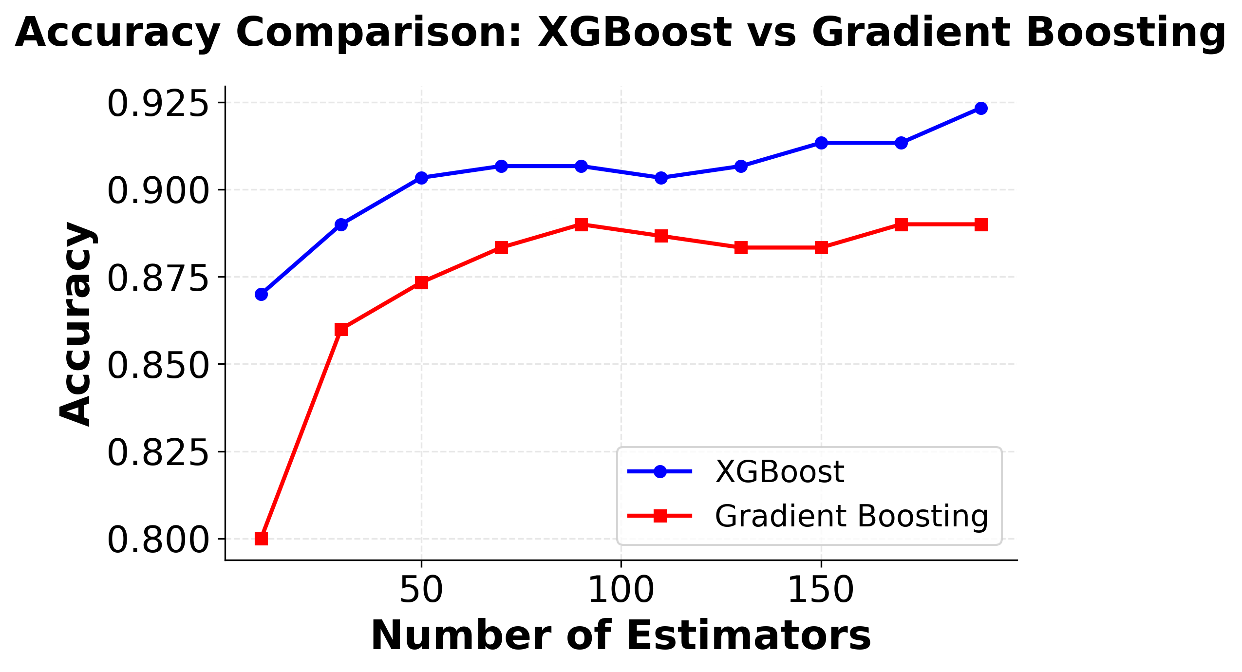
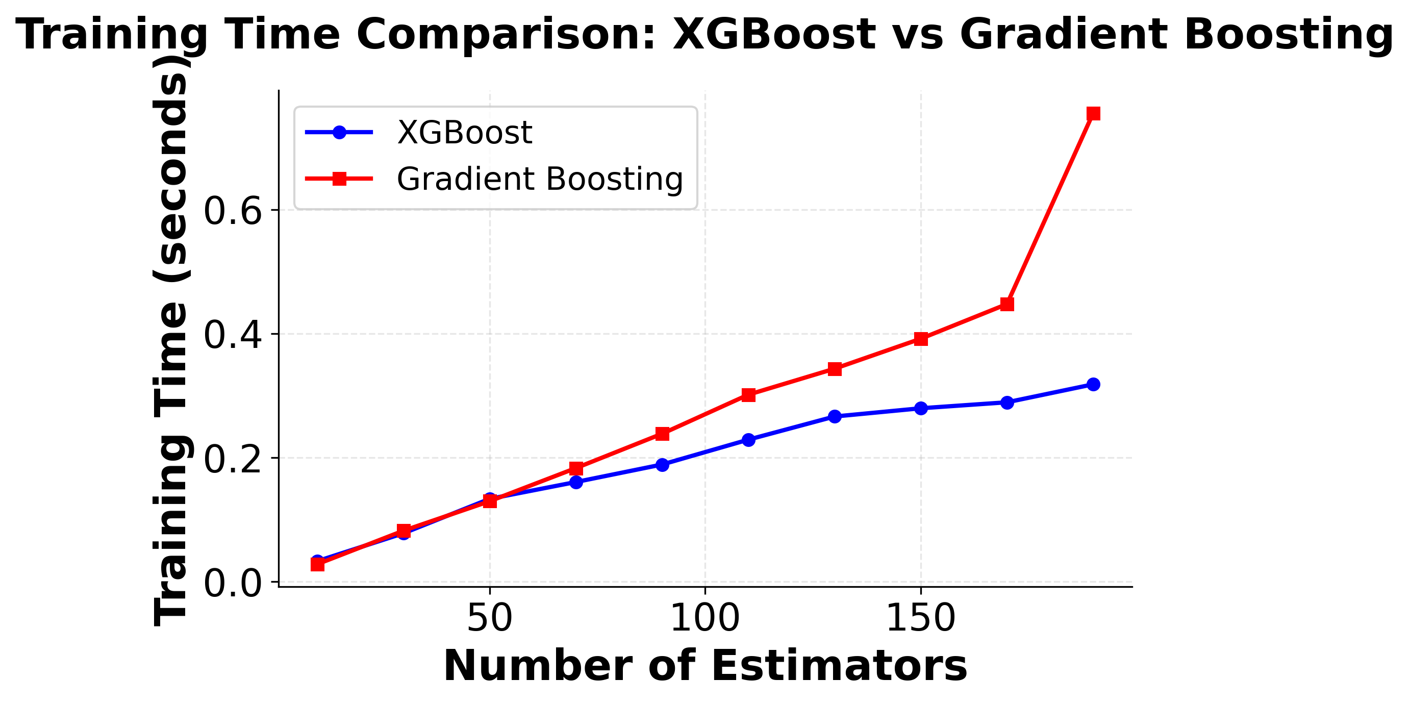
Here you can see XGBoost's superior performance characteristics compared to traditional gradient boosting. The left plot shows that XGBoost typically achieves higher accuracy with fewer estimators, while the right plot shows XGBoost's computational efficiency advantage, training significantly faster than traditional gradient boosting implementations.
Example
Let's work through a concrete example to demonstrate how XGBoost builds trees and makes predictions. We'll use a simple regression problem with a small dataset to make the calculations manageable.
Consider a dataset with 6 samples for predicting house prices based on two features: square footage (sqft) and number of bedrooms (bedrooms):
| Sample | sqft | bedrooms | Price (y) |
|---|---|---|---|
| 1 | 1000 | 2 | 200000 |
| 2 | 1200 | 3 | 250000 |
| 3 | 800 | 1 | 150000 |
| 4 | 1500 | 3 | 300000 |
| 5 | 1100 | 2 | 220000 |
| 6 | 1300 | 4 | 280000 |
We'll use mean squared error as our loss function: . The first and second derivatives are:
Step 1: Initialize with the mean We start by predicting the mean of all target values:
Step 2: Calculate gradients for the first tree For each sample, we calculate the gradient:
- Sample 1: ,
- Sample 2: ,
- Sample 3: ,
- Sample 4: ,
- Sample 5: ,
- Sample 6: ,
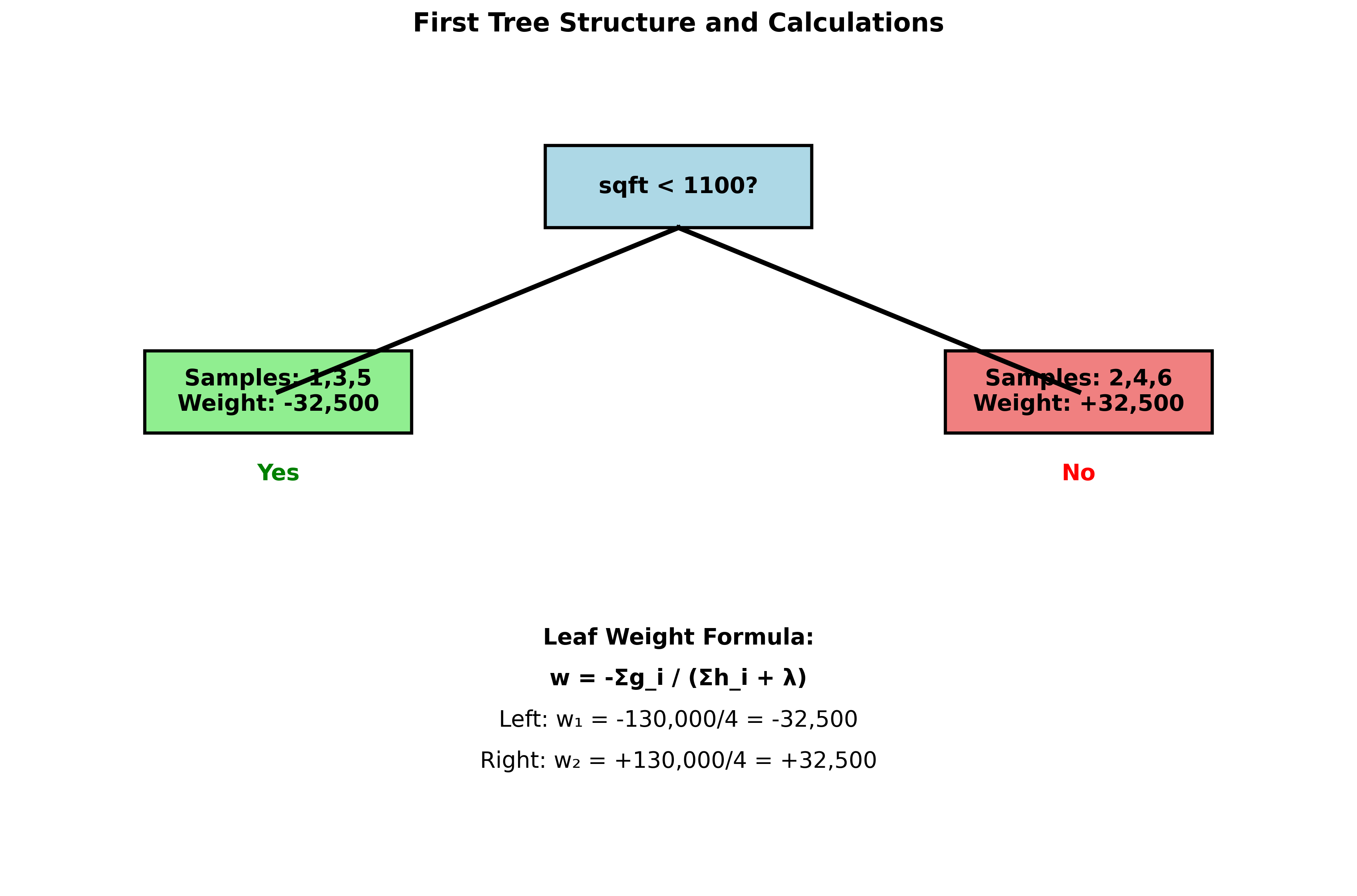
Step 3: Build the first tree Let's say we create a simple tree that splits on sqft < 1100:
- Left leaf (sqft < 1100): samples 1, 3, 5
- Right leaf (sqft ≥ 1100): samples 2, 4, 6
For the left leaf:
For the right leaf:
Note: The negative sign in the right leaf calculation comes from the fact that we're taking the negative of a negative sum, which results in a positive value. This reflects that samples in the right leaf (larger houses) need positive corrections to their predictions.
If we set (L2 regularization):
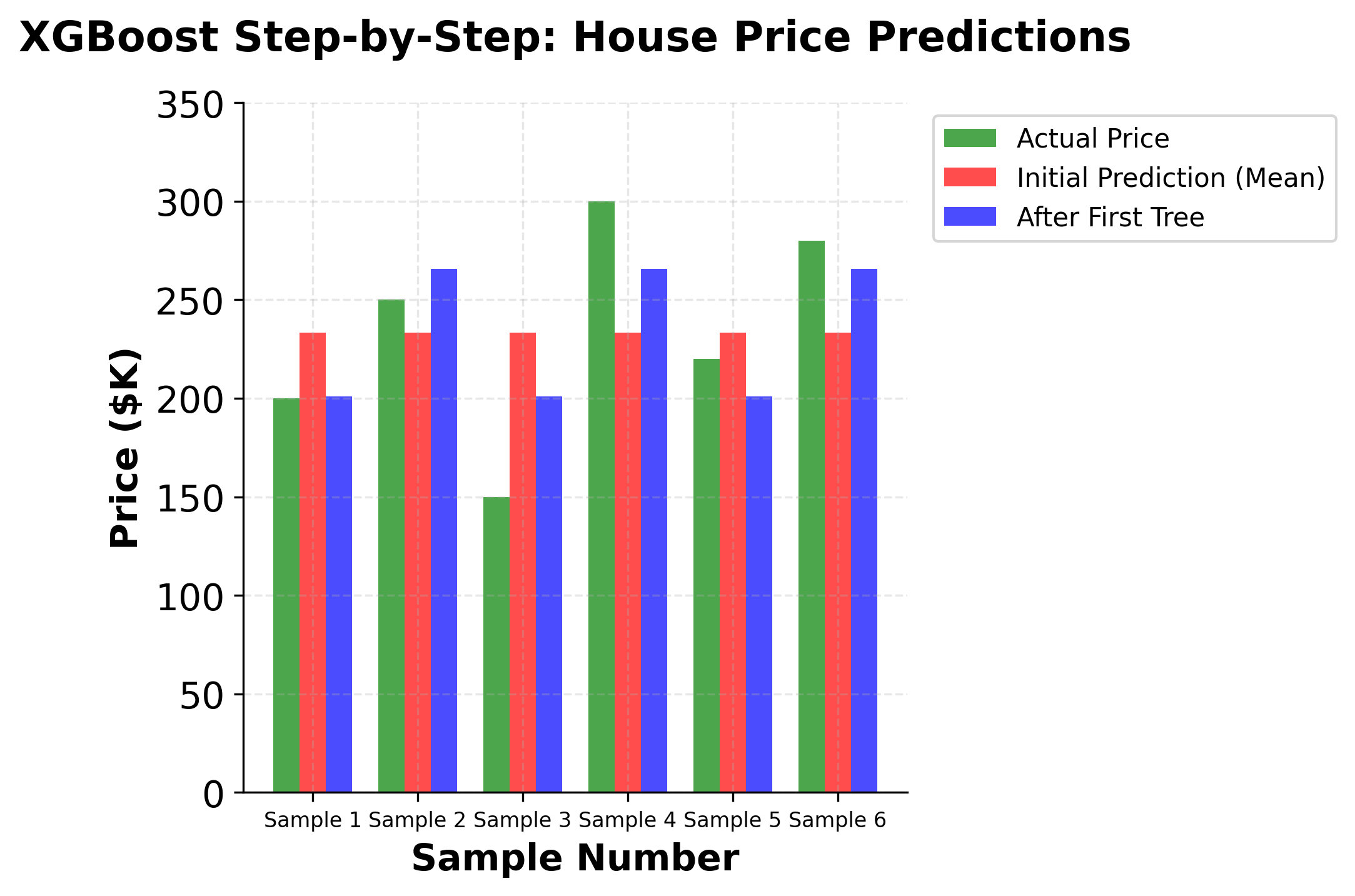
Step 4: Update predictions After the first tree:
- Sample 1:
- Sample 2:
- Sample 3:
- Sample 4:
- Sample 5:
- Sample 6:
We can see that the first tree has started to correct the initial predictions, moving them closer to the actual values. The process continues iteratively, with each subsequent tree focusing on the remaining prediction errors.
Ranking Example
Let's work through a concrete ranking example to demonstrate how XGBoost handles learning-to-rank problems. We'll use a search engine scenario where we want to rank documents for a given query.
Consider a query "machine learning tutorial" with 4 documents that need to be ranked:
| Document | Features | Relevance Score |
|---|---|---|
| Doc 1 | [0.8, 0.9, 0.7] | 3 (Highly relevant) |
| Doc 2 | [0.6, 0.5, 0.8] | 1 (Not relevant) |
| Doc 3 | [0.9, 0.8, 0.6] | 2 (Somewhat relevant) |
| Doc 4 | [0.7, 0.7, 0.9] | 2 (Somewhat relevant) |
Step 1: Initialize predictions We start with initial predictions (typically zeros or small random values):
- Doc 1:
- Doc 2:
- Doc 3:
- Doc 4:
Step 2: Calculate pairwise ranking loss For the pairwise ranking loss, we consider all pairs where one document should be ranked higher than another based on relevance scores.
Relevant pairs (Doc i should rank higher than Doc j):
- (Doc 1, Doc 2): relevance 3 > 1
- (Doc 1, Doc 3): relevance 3 > 2
- (Doc 1, Doc 4): relevance 3 > 2
- (Doc 3, Doc 2): relevance 2 > 1
- (Doc 4, Doc 2): relevance 2 > 1
The pairwise loss for each pair is:
Since all initial predictions are 0, the loss for each pair is:
Step 3: Calculate gradients for ranking For ranking problems, the gradient calculation is more complex as it involves the pairwise relationships. The gradient for document is:
With initial predictions of 0, this simplifies to:
- Doc 1: (should rank higher than 3 docs)
- Doc 2: (should rank lower than 3 docs)
- Doc 3: (should rank higher than 1, lower than 1)
- Doc 4: (should rank higher than 1, lower than 1)
Step 4: Build the first ranking tree Let's say we create a tree that splits on the first feature < 0.75:
- Left leaf (feature 1 < 0.75): Doc 2, Doc 4
- Right leaf (feature 1 ≥ 0.75): Doc 1, Doc 3
For the left leaf:
For the right leaf:
With :
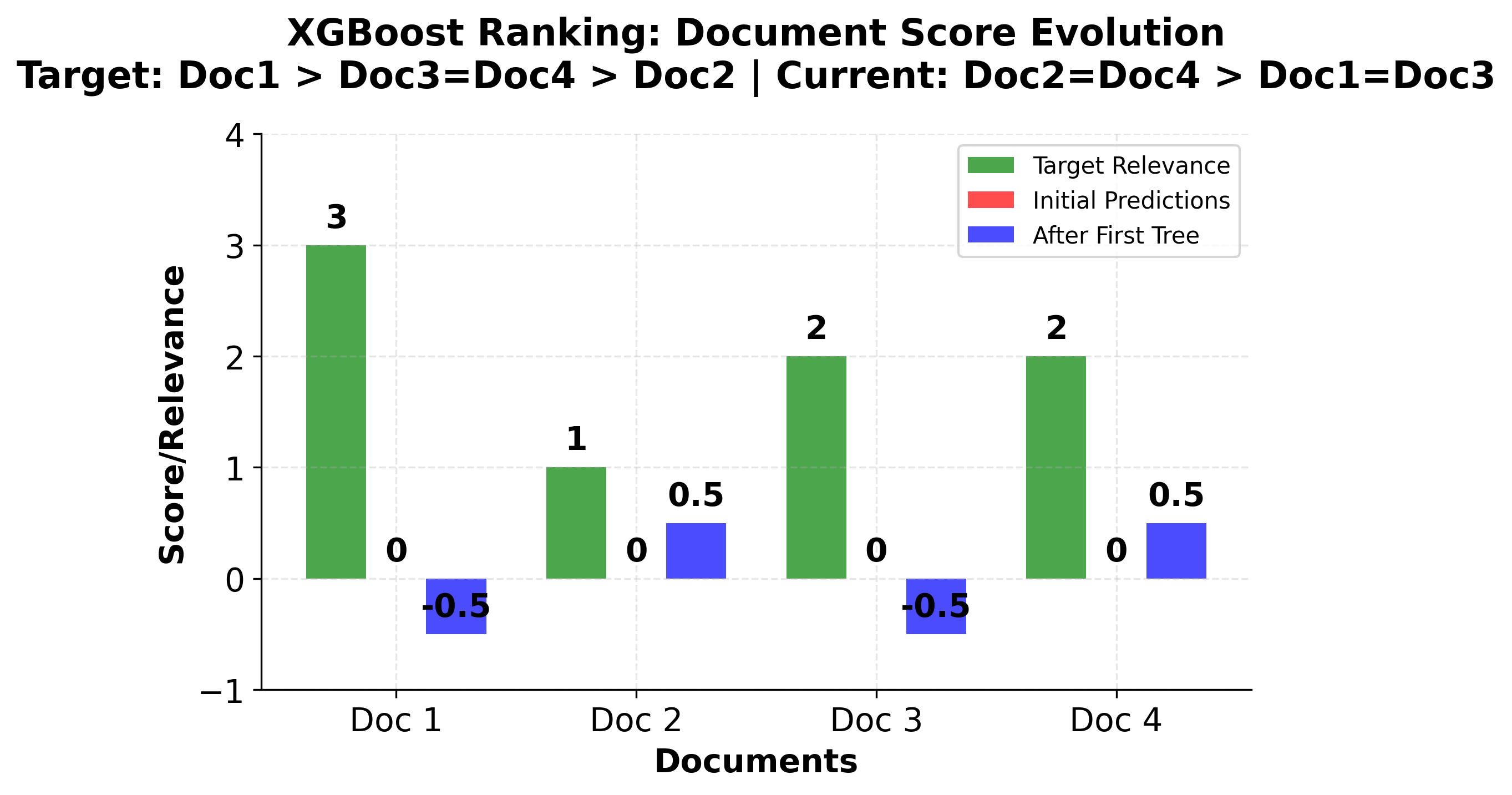
Step 5: Update predictions After the first tree:
- Doc 1:
- Doc 2:
- Doc 3:
- Doc 4:
The ranking after the first tree is: Doc 2, Doc 4 (tied), Doc 1, Doc 3 (tied). This is not the correct ranking yet, so subsequent trees will continue to refine the predictions to achieve the desired ranking order.
Implementation using XGBoost by DMLC
XGBoost can be implemented using the scikit-learn compatible XGBoost library, which provides a familiar interface while leveraging XGBoost's advanced optimization features. Let's demonstrate this with both classification and regression examples.
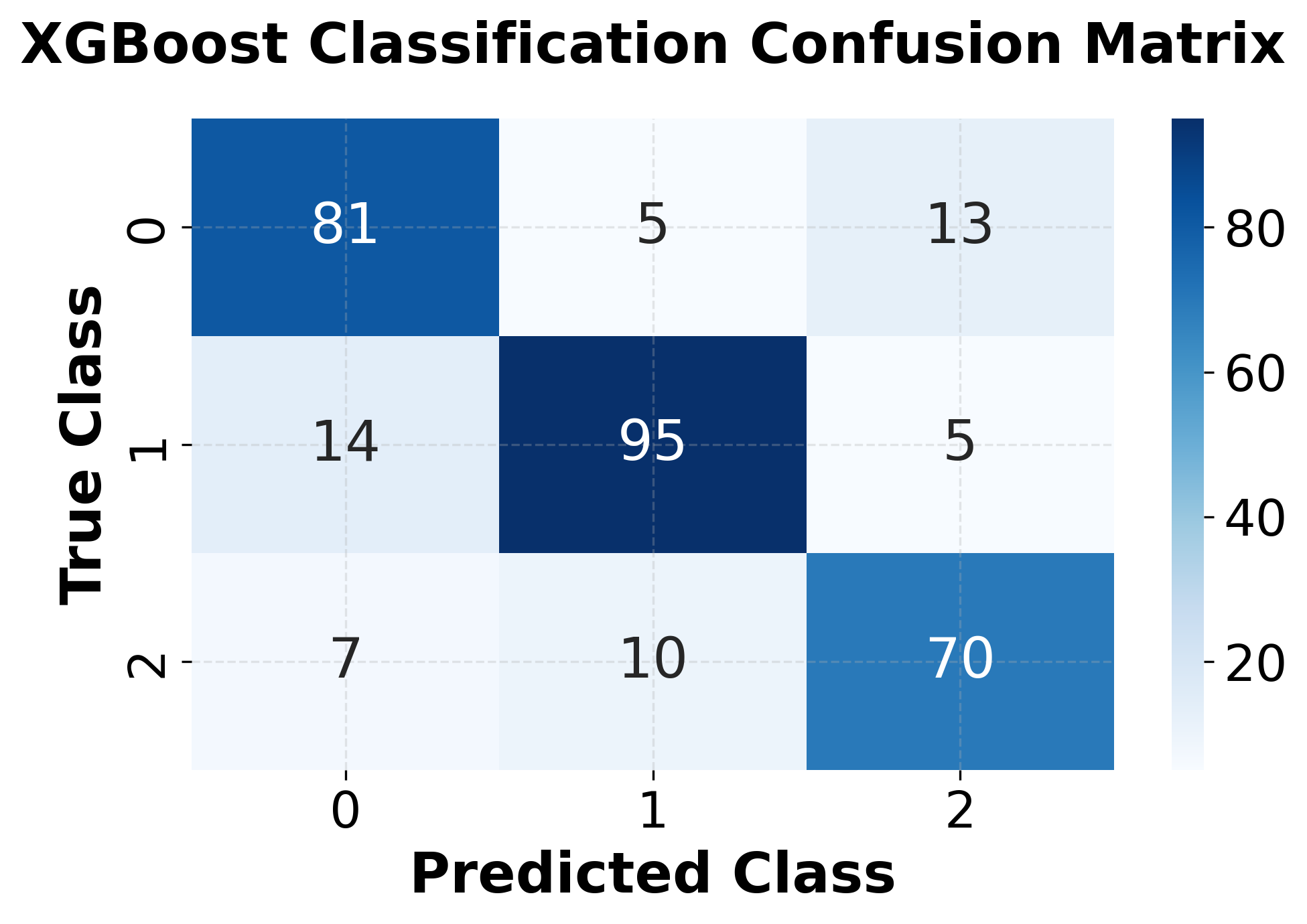
Classification Example
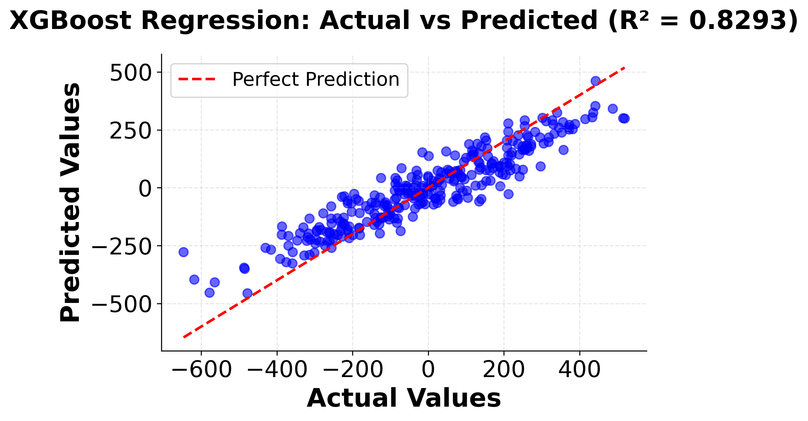
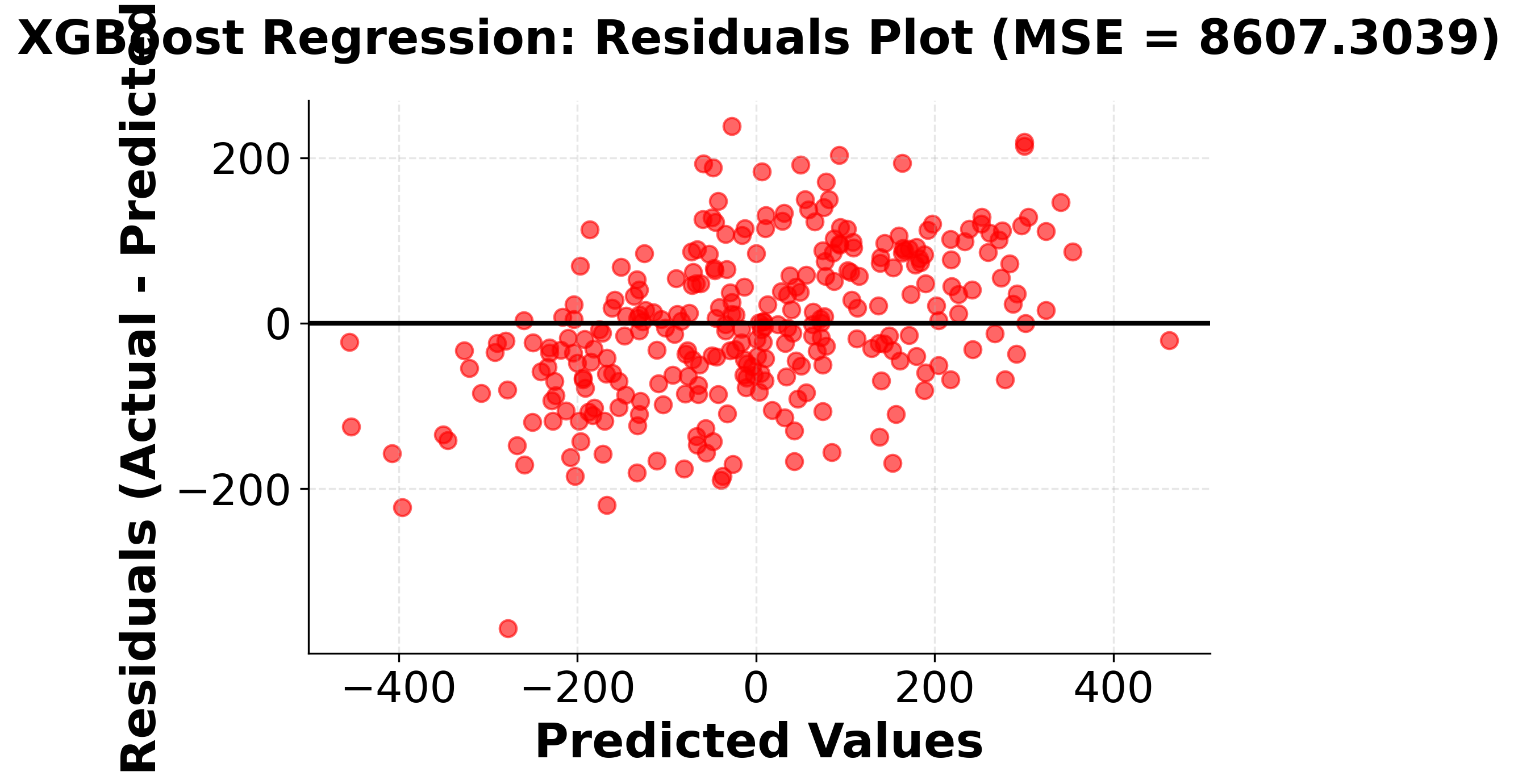
Regression Example
Hyperparameter Tuning Example
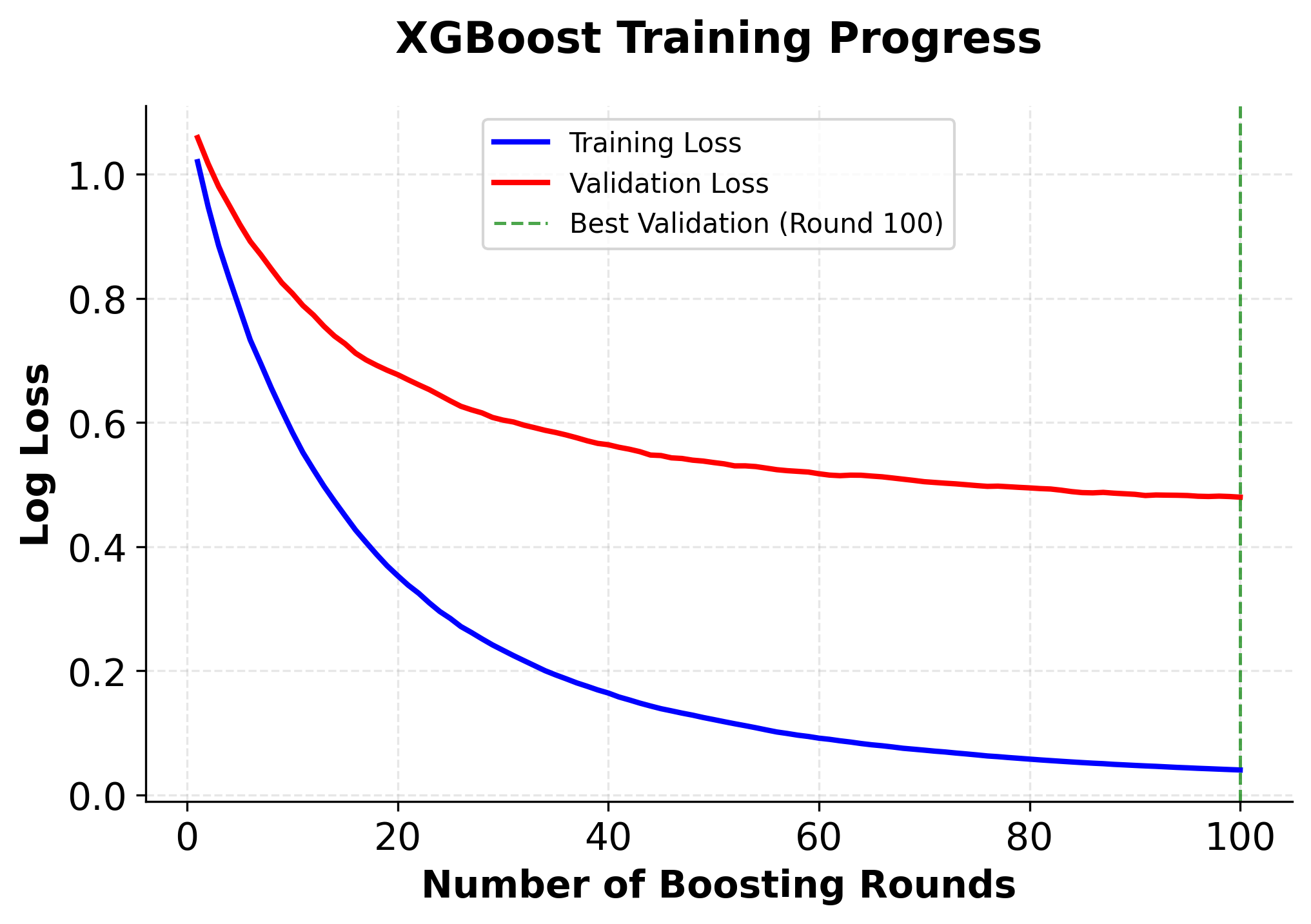
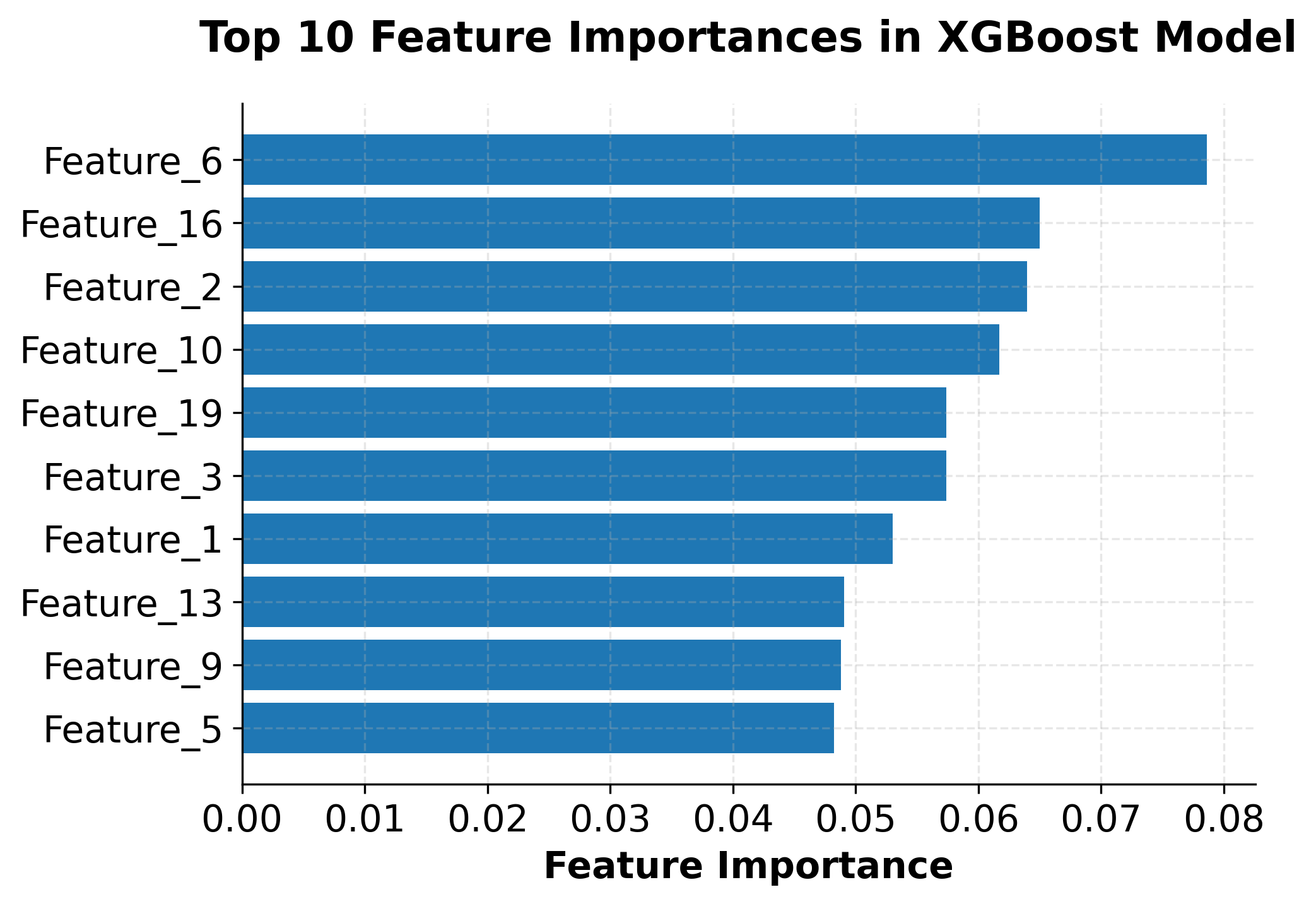
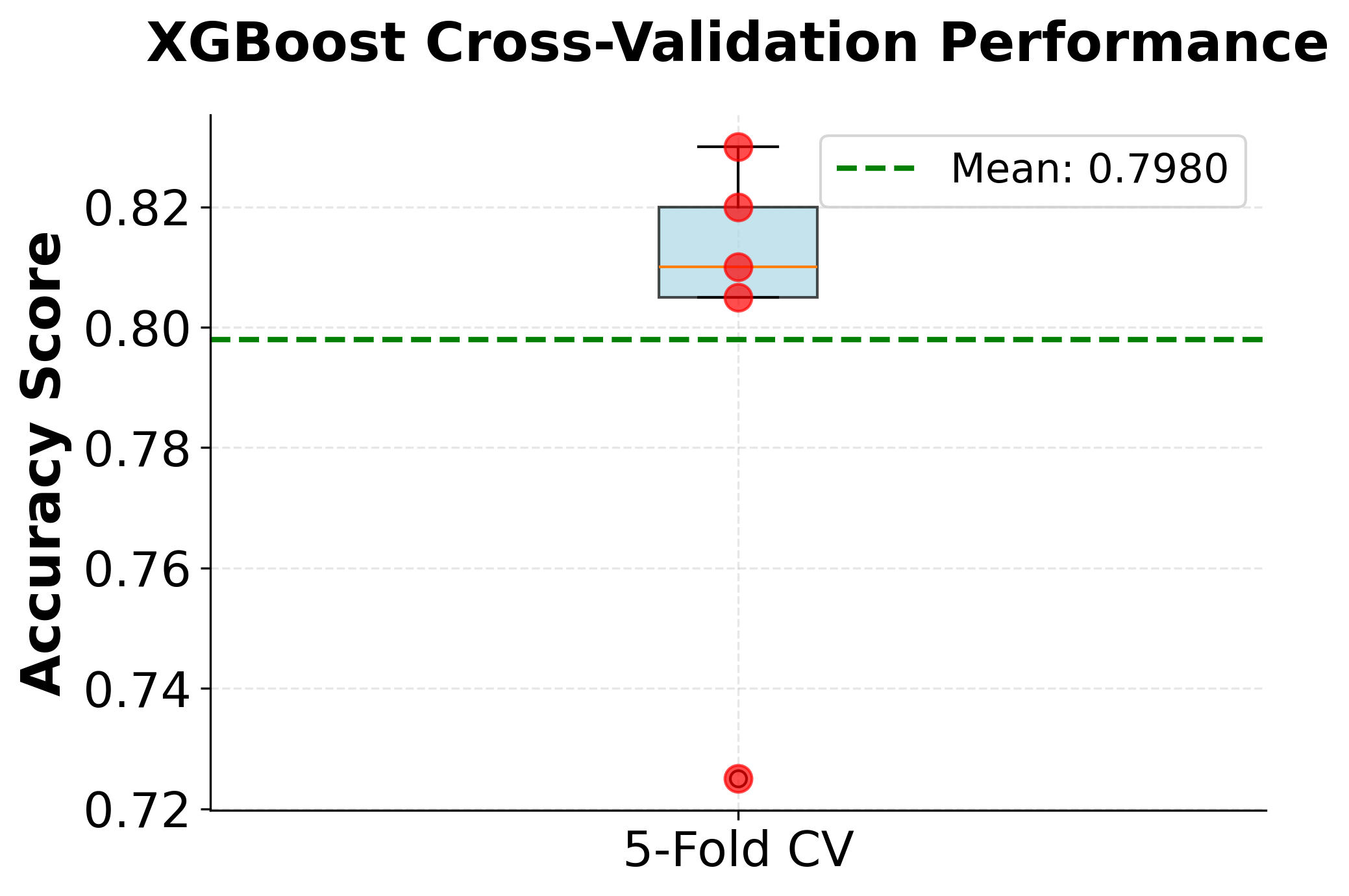
The implementation demonstrates several key aspects of using XGBoost in practice. The scikit-learn compatible interface makes it easy to integrate XGBoost into existing machine learning workflows, while the extensive hyperparameter options allow for fine-tuning performance. The feature importance analysis shows how XGBoost can help identify the most relevant features in the dataset, which is valuable for both model interpretation and feature selection.
Key takeaways from this implementation:
- XGBoost provides excellent out-of-the-box performance with minimal tuning
- The algorithm handles both classification and regression tasks effectively
- Hyperparameter tuning can significantly improve performance
- Feature importance analysis provides valuable insights into the model's decision-making process
Ranking Implementation Example
XGBoost also supports learning-to-rank tasks, which are crucial for applications like search engines, recommendation systems, and information retrieval. Let's demonstrate how to implement ranking with XGBoost.
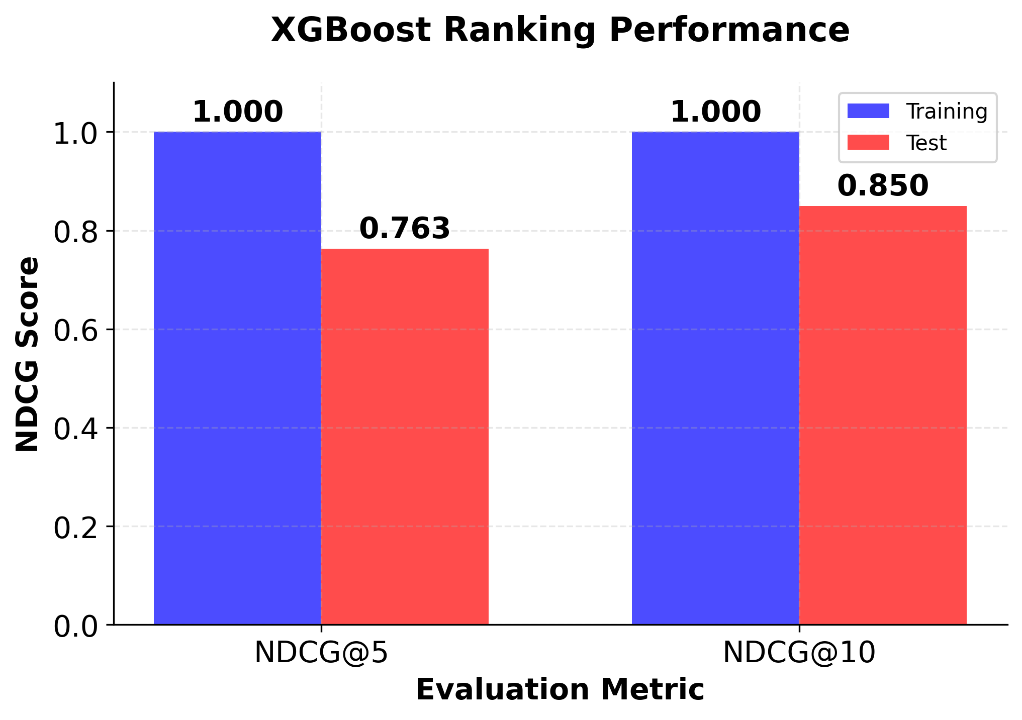
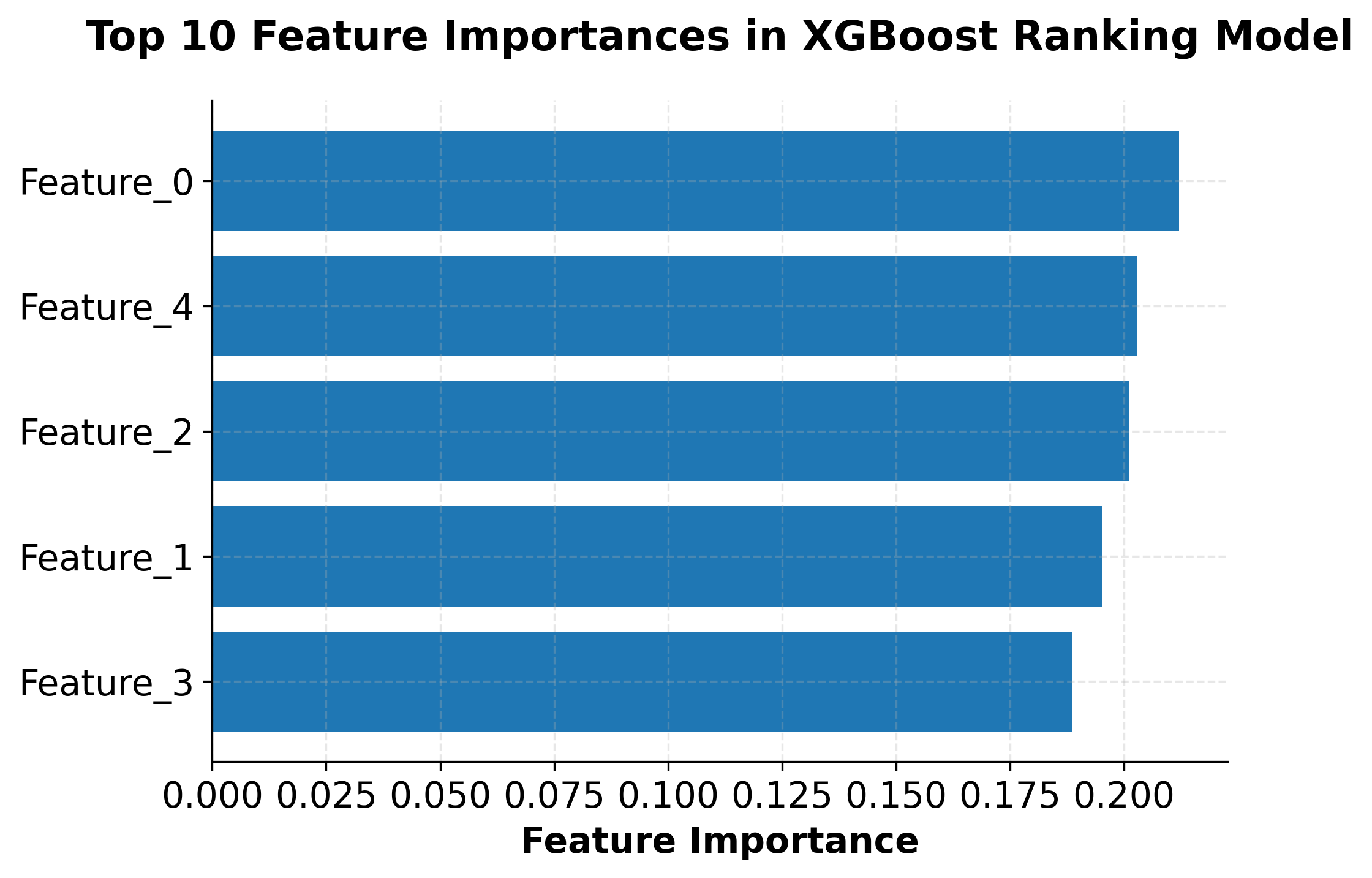
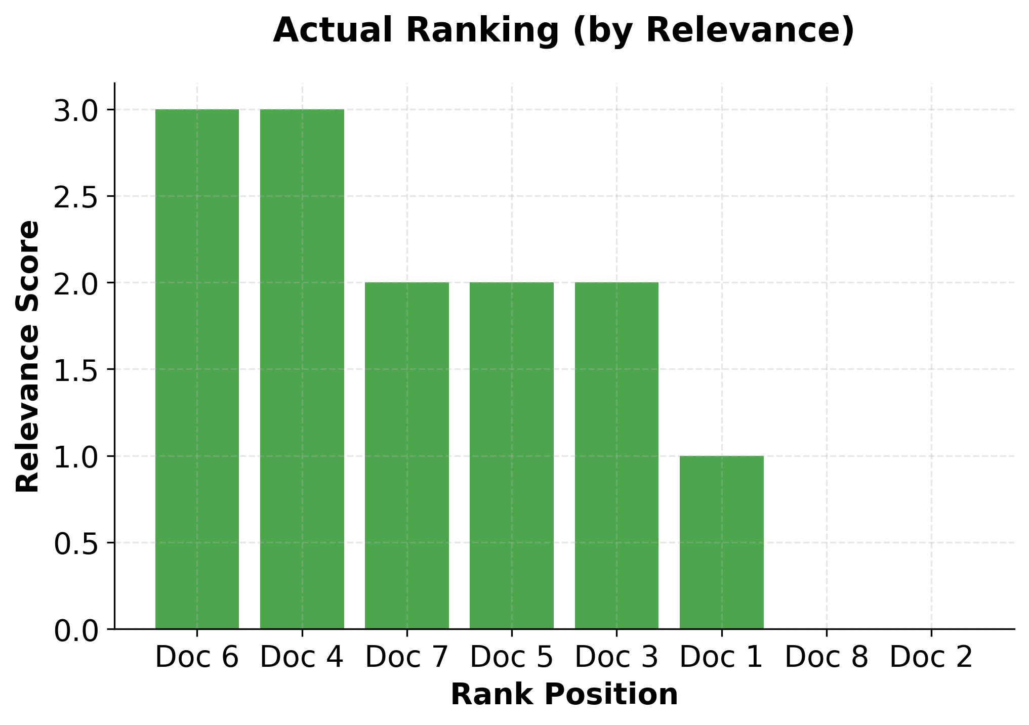
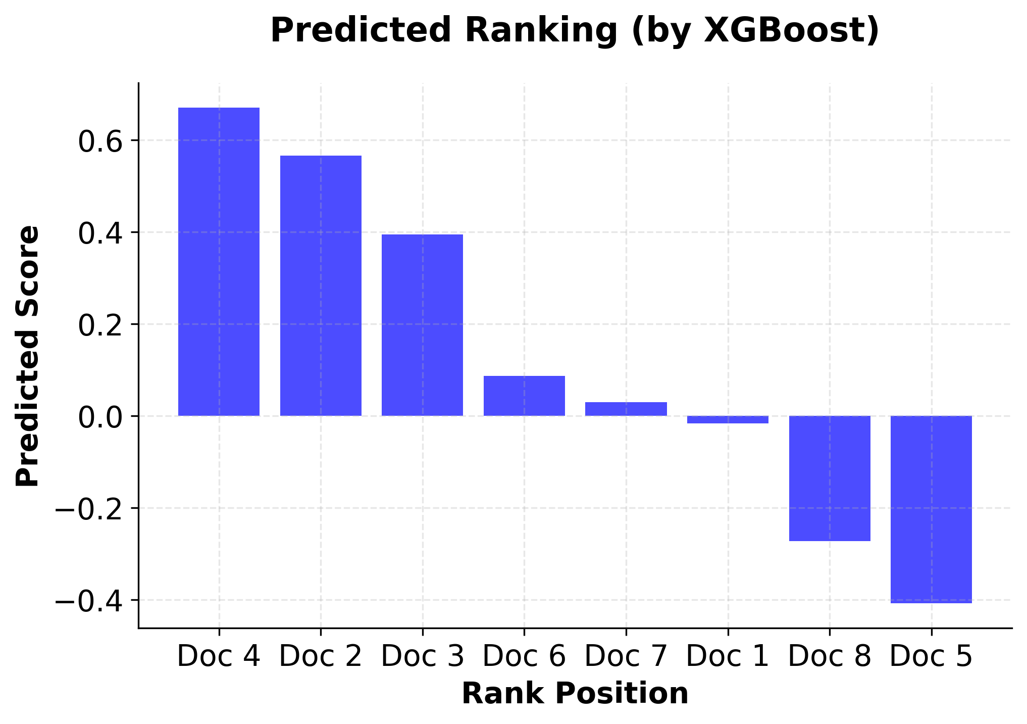
The ranking implementation demonstrates XGBoost's capability to handle learning-to-rank problems effectively. Key aspects of this implementation include:
- Group-based training: XGBoost uses query groups to understand which documents belong to the same query
- Pairwise ranking objective: The model optimizes for correct pairwise document ordering
- NDCG evaluation: Standard ranking metrics are used to assess performance
- Feature importance: Understanding which features contribute most to ranking decisions
This makes XGBoost particularly valuable for applications like search engines, recommendation systems, and any scenario where relative ordering of items is more important than absolute scores.
Practical implications
XGBoost excels in several specific scenarios and use cases where its unique combination of performance, efficiency, and flexibility provides significant advantages. Understanding when to choose XGBoost over alternatives like LightGBM or CatBoost is crucial for optimal model selection.
When to choose XGBoost over LightGBM: XGBoost is often the better choice when you need maximum predictive accuracy and have sufficient computational resources. It typically performs better on smaller to medium-sized datasets (up to several million samples) where the computational overhead is manageable. XGBoost's more conservative approach to tree building often leads to better generalization, making it preferable for applications where model stability and reliability are critical, such as financial modeling, medical diagnosis, or any domain where prediction errors have significant consequences.
When to choose XGBoost over CatBoost: XGBoost is generally preferred when you have well-preprocessed numerical data and want more control over the training process. While CatBoost excels with categorical features and requires minimal preprocessing, XGBoost offers more flexibility in hyperparameter tuning and model customization. If you need to implement custom loss functions or have specific regularization requirements, XGBoost's extensive configuration options make it the better choice.
Data requirements and preprocessing: XGBoost works best with numerical data and requires careful handling of categorical variables through encoding techniques like one-hot encoding or label encoding. The algorithm is relatively robust to missing values and can handle them automatically, but explicit preprocessing often leads to better results. Feature scaling is generally not required for tree-based methods, but ensuring that features are on similar scales can help with hyperparameter tuning.
Computational considerations: XGBoost's memory usage scales with the number of features and samples, making it suitable for datasets that fit in memory. For very large datasets (tens of millions of samples), LightGBM might be more appropriate due to its memory efficiency. However, XGBoost's parallel processing capabilities make it well-suited for multi-core systems, and it can leverage GPU acceleration for even faster training on compatible hardware.
Industry applications: XGBoost has proven particularly successful in domains requiring high accuracy and interpretability, including finance (credit scoring, fraud detection), healthcare (diagnosis, drug discovery), e-commerce (recommendation systems, pricing optimization), and manufacturing (quality control, predictive maintenance). Its ability to handle mixed data types and provide feature importance rankings makes it valuable for exploratory data analysis and feature engineering workflows.
Ranking applications: XGBoost's ranking capabilities make it particularly valuable for learning-to-rank applications. In search engines, XGBoost can effectively rank web pages based on query relevance, combining features like text similarity, page authority, and user engagement metrics. Recommendation systems benefit from XGBoost's ability to rank items for individual users, optimizing for both relevance and diversity. Information retrieval systems use XGBoost to rank documents, articles, or products based on user queries and contextual information. The algorithm's support for group-based training makes it well-suited for scenarios where items need to be ranked within specific contexts or queries.
Scaling and deployment considerations: For production deployment, XGBoost models are relatively lightweight and can be easily serialized and deployed using standard machine learning serving frameworks. The algorithm's deterministic nature (with fixed random seeds) ensures reproducible results, which is crucial for production systems. However, the computational requirements for training can be significant, so consider using cloud computing resources or distributed training for large-scale applications.
Summary
XGBoost represents a sophisticated evolution of gradient boosting that has become one of the most successful machine learning algorithms in practice. By incorporating second-order gradient information, advanced regularization techniques, and highly optimized computational implementations, XGBoost achieves superior predictive performance while maintaining computational efficiency. The algorithm's mathematical foundation builds upon traditional gradient boosting but introduces key innovations that enable faster convergence and better generalization.
The practical advantages of XGBoost make it an excellent choice for a wide range of machine learning applications, particularly when accuracy and model interpretability are priorities. Its flexibility in handling various data types, comprehensive hyperparameter options, and robust feature importance analysis capabilities make it valuable for both prediction and exploratory analysis. The algorithm's support for ranking tasks through specialized loss functions and group-based training makes it particularly powerful for learning-to-rank applications in search engines, recommendation systems, and information retrieval.
While the algorithm requires careful hyperparameter tuning and can be computationally intensive, the resulting performance gains often justify the additional effort. XGBoost's ability to handle classification, regression, and ranking tasks with the same underlying framework provides practitioners with a versatile tool that can address diverse machine learning challenges.
When choosing between XGBoost and alternatives like LightGBM or CatBoost, the decision should be based on specific requirements around accuracy, computational resources, data characteristics, and deployment constraints. XGBoost excels in scenarios where maximum predictive performance is needed and computational resources are available, making it particularly suitable for applications in finance, healthcare, search engines, and other domains where prediction accuracy is critical. The algorithm's continued success in machine learning competitions and production systems demonstrates its effectiveness as a powerful tool for modern data science applications.
Quiz
Ready to test your understanding of XGBoost? Take this quiz to reinforce what you've learned about this powerful gradient boosting algorithm.

Comments