

Build a robust quantitative research pipeline. From hypothesis formulation and backtesting to paper trading and live production deployment strategies.
Choose your expertise level to adjust how many terms are explained. Beginners see more tooltips, experts see fewer to maintain reading flow. Hover over underlined terms for instant definitions.
Research Pipeline and Strategy Deployment
The journey from a trading idea to a live, profit-generating strategy is rarely straightforward. Many promising concepts fail not because they lack merit, but because the process of developing, testing, and deploying them was flawed. Ad-hoc research leads to overfitting, unreproducible results, and costly surprises when strategies encounter live markets. A disciplined research pipeline transforms this chaotic process into a systematic workflow where each step builds confidence that a strategy will perform as expected in production.
This chapter walks you through the complete lifecycle of a quantitative trading strategy. We begin with the research workflow, covering how to formulate testable hypotheses, gather and clean data, build models, and iterate toward robust strategies. We then explore version control and experiment tracking, essential practices for maintaining reproducibility when testing dozens of parameter combinations across multiple strategy variants. Paper trading, the final validation step before risking real capital, reveals implementation issues that backtests cannot catch. Finally, we cover production deployment, including scheduling, monitoring, alerting, and the ongoing evaluation that determines when a strategy needs recalibration or retirement.
Building on the backtesting framework from Chapter 1 of this part, the transaction cost models from Chapter 2, and the infrastructure concepts from Chapter 5, this chapter integrates these components into a cohesive system that takes strategies from conception to continuous operation.
The Research Workflow
Successful quantitative research follows a structured process that balances creativity with rigor. Each stage has specific objectives and quality gates that a strategy must pass before advancing to the next phase. Think of this workflow as a funnel: many ideas enter at the top, but only those that survive increasingly demanding tests emerge at the bottom ready for live trading. This disciplined approach protects capital by ensuring that only thoroughly vetted strategies receive real money.
Hypothesis Formulation
Every trading strategy begins with a hypothesis about market behavior. This hypothesis should be specific, testable, and grounded in economic reasoning. Vague ideas like momentum works are insufficient because they provide no guidance on implementation and no criteria for determining success or failure. Instead, formulate precise statements such as "stocks in the top decile of 12-month returns, excluding the most recent month, outperform the bottom decile by 0.5% per month over the subsequent three months, with this effect being stronger in small-cap stocks."
The precision of this formulation serves multiple purposes:
- Specificity: It specifies exactly what you will measure, eliminating ambiguity that might otherwise lead to post-hoc rationalization of results.
- Success Criterion: It provides a clear success criterion. If the observed effect is substantially smaller than 0.5% per month, you know the hypothesis has failed.
- Validation: It identifies auxiliary predictions (stronger in small caps) that can serve as additional validation, since a genuine effect should exhibit predictable patterns while a spurious correlation typically will not.
A testable statement about market behavior that specifies the asset universe, the signal or factor being tested, the expected effect size, the holding period, and any conditions under which the effect should be stronger or weaker.
Strong hypotheses share several characteristics:
- Economic Rationale: They explain why the effect should exist and persist. Effects with clear economic explanations tend to be more robust than statistical patterns without theoretical grounding.
- Expected Magnitude: They specify the expected size of the effect, allowing you to determine whether transaction costs would erode potential profits. A hypothesis predicting a 0.1% monthly return is fundamentally different from one predicting 1%, even if both turn out to be statistically significant.
- Conditions: They identify conditions that might strengthen or weaken the signal, providing out-of-sample tests of the underlying mechanism. If you believe momentum works because of investor underreaction to news, then you should predict stronger momentum effects following information events.
The structured hypothesis clearly defines the signal, universe, and expected outcome. This specificity allows for precise testing and ensures that the strategy's success or failure can be measured against concrete expectations rather than vague intuitions. Notice how each field in the hypothesis documentation serves a purpose: the asset universe constrains where you look, the signal definition specifies exactly what you calculate, the expected effect provides a benchmark for success, and the economic rationale explains why you believe this pattern should persist rather than being a historical accident.
Data Gathering and Cleaning
With a hypothesis in hand, you need data to test it. Data quality issues are the most common source of misleading backtest results. As we discussed in Chapter 9 of Part I on data handling, financial data requires careful attention to survivorship bias, look-ahead bias, and corporate actions.
The challenge with financial data is that errors are often subtle and systematic. A database that only includes currently listed stocks excludes all the companies that went bankrupt or were delisted, creating survivorship bias that inflates backtest returns. Price data that has not been adjusted for stock splits can show apparent 50% daily returns that never actually occurred. Dividend data that arrives with a one-day lag can cause look-ahead bias if your backtest uses it on the ex-dividend date. These issues do not announce themselves; you must actively search for them.
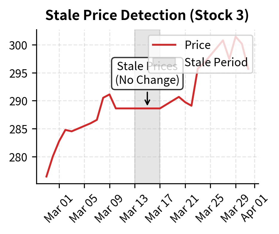
The quality report identifies specific data issues that could compromise backtest validity. The presence of missing data and stale prices indicates that the dataset requires cleaning steps, such as forward-filling prices or excluding affected assets, before it can be used for reliable signal generation. Each warning in this report represents a potential source of bias: stale prices might indicate delisted securities whose final decline is not captured, while extreme returns could be data errors that would artificially boost or harm strategy performance.
Feature Engineering and Signal Construction
Once you have clean data, construct the signals that will drive trading decisions. Feature engineering transforms raw price and volume data into predictive signals. As we covered in Chapter 8 of Part VI on machine learning techniques, features should capture meaningful market dynamics without introducing look-ahead bias.
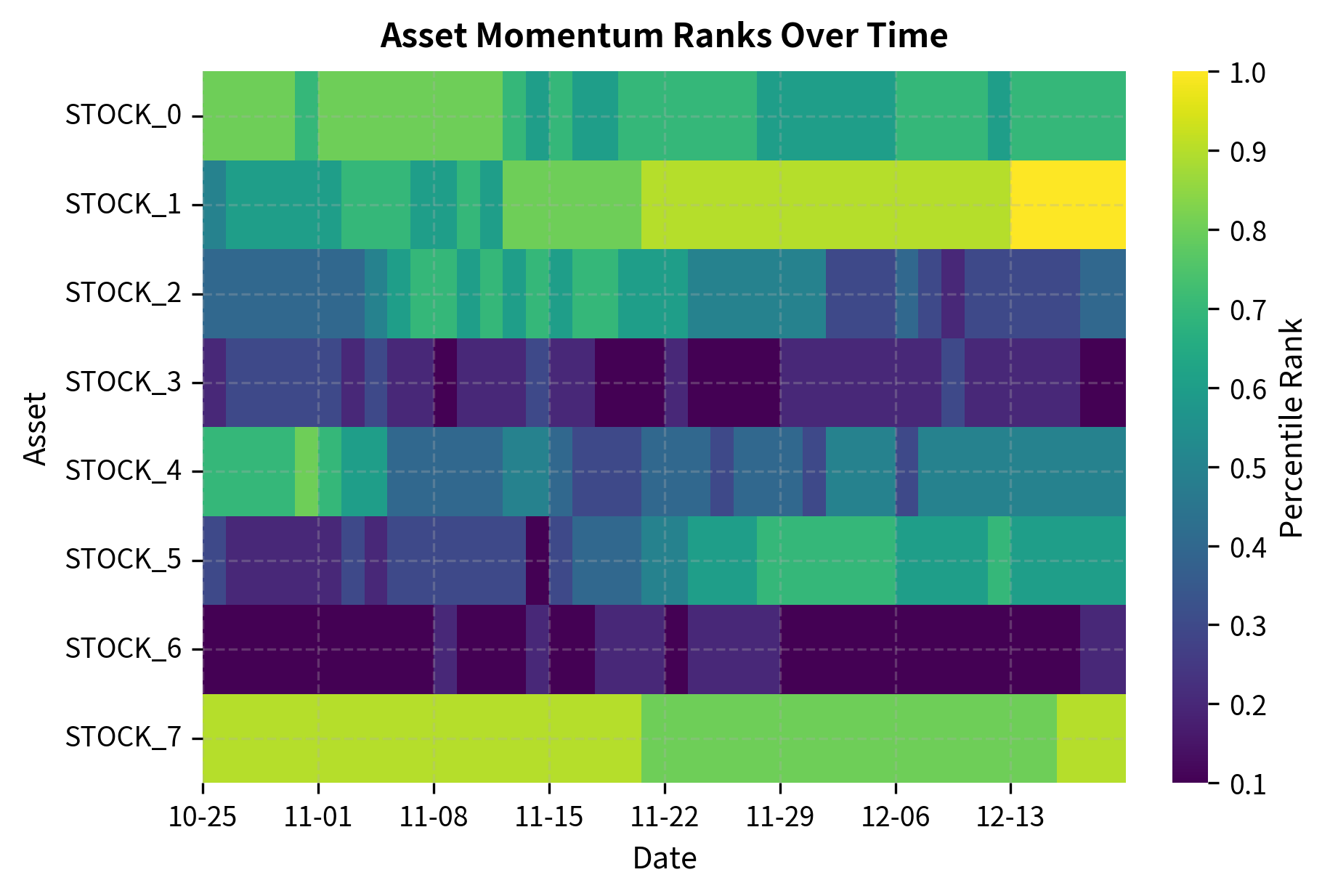
The art of signal construction lies in translating an economic hypothesis into a mathematical formula. Consider momentum: the hypothesis states that past winners continue to outperform. But "past winners" requires precise definition. Over what period do we measure past performance? Do we include the most recent days, or does short-term reversal contaminate the signal? Should we adjust for volatility, so that a 20% return in a low-volatility stock is treated differently from a 20% return in a high-volatility stock? Each of these choices reflects an assumption about the underlying mechanism, and the best choices come from understanding the economics rather than from optimization.
The statistics confirm that the cross-sectional ranking has normalized the signals to a consistent range. Both momentum and mean reversion signals now exhibit similar distributions, which prevents the strategy optimizer from being biased toward the signal with the larger raw magnitude. This normalization step is crucial when combining multiple signals: without it, the signal with the largest variance would dominate the combined forecast simply due to its scale rather than its predictive power.
Signal Parameters
Understanding the key parameters in signal generation is essential for building robust trading strategies. Each parameter embodies a specific assumption about market behavior, and choosing appropriate values requires balancing responsiveness against noise reduction.
The lookback parameter determines the window size for calculating returns. This choice reflects your hypothesis about the persistence of the underlying effect. Longer lookbacks, such as 252 days representing one trading year, capture secular trends and filter out short-term noise. They are appropriate when you believe the effect operates over extended periods, as with traditional momentum strategies based on gradual information diffusion. Shorter lookbacks, such as 63 days representing one quarter, react faster to regime changes and capture more transient patterns. The tradeoff is clear: longer windows provide more stable signals but may miss turning points, while shorter windows adapt quickly but generate more false signals.
The skip parameter specifies the number of recent days excluded from the momentum calculation. This parameter addresses a well-documented empirical phenomenon: very short-term returns tend to reverse rather than persist. A stock that rose sharply over the past week often falls back over the subsequent week, contaminating the momentum signal with mean-reversion noise. By excluding the most recent 21 trading days (approximately one month), we isolate the medium-term persistence effect from the short-term reversal effect. Research has shown that this "12-1 momentum" formulation significantly outperforms naive 12-month momentum.
The vol_lookback parameter determines the period used to calculate volatility for signal normalization. When we divide momentum by volatility, we are measuring returns in units of risk rather than raw percentage points. A 20% return for a stock with 15% annual volatility represents a much stronger signal than a 20% return for a stock with 60% annual volatility. The vol_lookback should be long enough to provide a stable volatility estimate but short enough to capture changes in the risk environment. A 63-day (quarterly) window typically provides a good balance, smoothing out daily noise while remaining responsive to persistent volatility shifts.
Research Iteration and Validation
Research is inherently iterative. Initial results rarely support the hypothesis as strongly as hoped, and the temptation to adjust parameters until results look good leads to overfitting. A disciplined approach separates exploration from confirmation.
The danger of iteration is subtle but severe. Each time you test a parameter combination and observe its performance, you gain information. If you then use that information to select parameters, you are implicitly fitting to the specific historical dataset. Run enough tests, and some combination will look good by chance alone. The solution is to maintain a clear distinction between exploratory research, where you try many ideas freely, and confirmatory research, where you test a pre-specified hypothesis on held-out data. The experiment log below helps enforce this discipline by creating a record of what you tested and why.
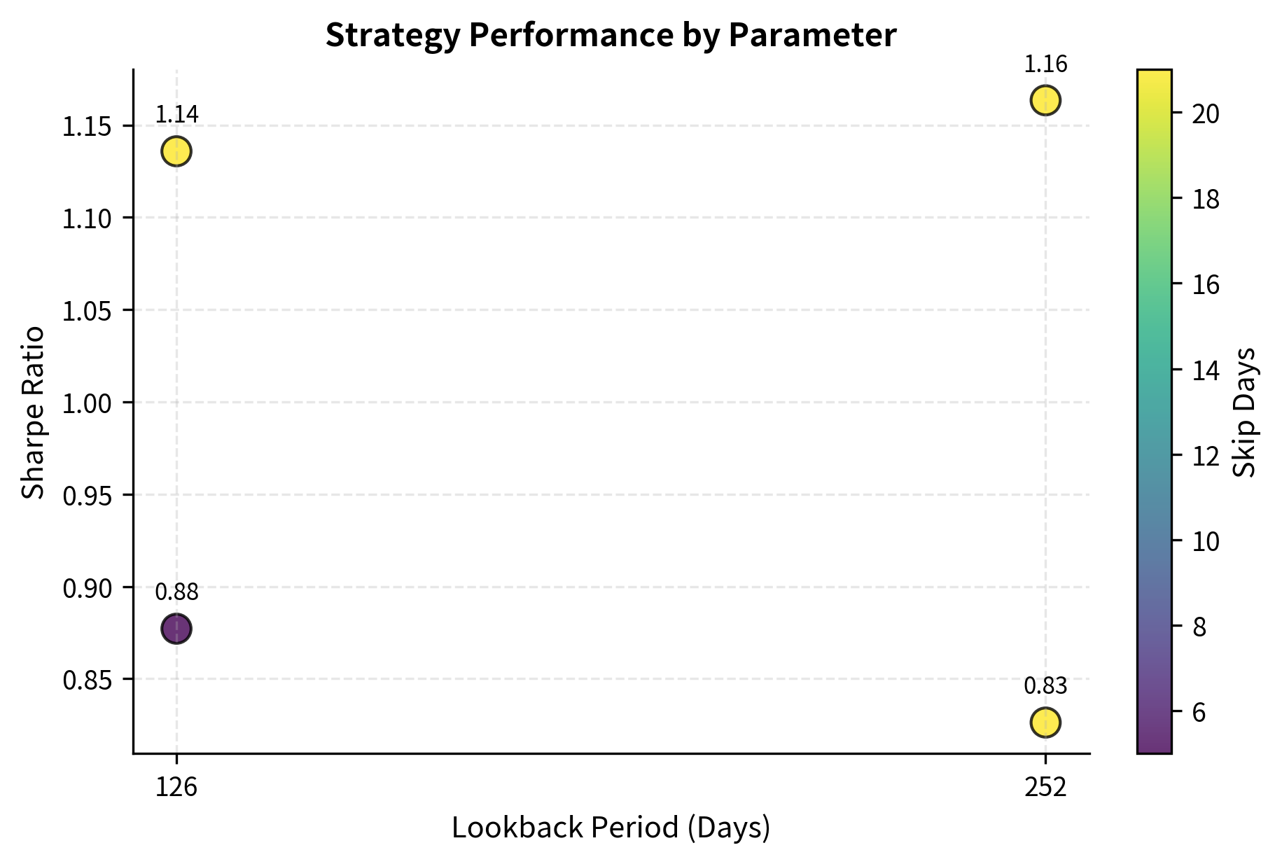
The experiment log allows us to compare performance across different parameter sets. In this simulation, the configuration with a 252-day lookback yields the highest Sharpe ratio, suggesting that the underlying momentum effect is stronger over longer time horizons in this dataset. However, note the importance of not simply selecting the best-performing parameters: the right approach is to use this information to generate hypotheses that you then test on held-out data. If longer lookbacks consistently outperform across multiple samples, that pattern is more likely to persist than a single lucky result.
Version Control and Experiment Tracking
As research progresses, you accumulate hundreds of experiments across multiple strategy variants. Without systematic tracking, reproducing results becomes impossible, and you lose the ability to understand what worked and why.
Git for Code Versioning
Version control with Git is foundational. Every change to strategy code, data processing pipelines, and configuration files should be tracked. A well-organized repository structure separates concerns and makes collaboration easier.
The repository structure below reflects a principle of separation of concerns: data handling lives in one place, signal generation in another, and execution logic in a third. This separation ensures that a bug fix in execution code cannot accidentally break signal calculation. It also enables different team members to work on different components simultaneously without creating merge conflicts. The notebooks directory provides a space for exploratory analysis, while the src directory contains production-quality code that has been tested and reviewed.
This structure clearly separates data, source code, and experimental notebooks. Placing reusable logic in the src directory ensures that both notebooks and production scripts import the same tested code, preventing logic divergence. The tests directory is not optional: automated tests catch regressions before they reach production. The experiments directory separates configuration files, which should be version controlled, from output files, which are often too large and numerous to store in Git.
Experiment Tracking with MLflow
While Git tracks code, experiment tracking tools like MLflow capture the full context of each run, including parameters, metrics, artifacts, and environment details. This enables comparing experiments across different code versions and parameter combinations.
The value of experiment tracking becomes apparent when you need to reproduce a result from six months ago. With only Git, you would know what code was committed but not which specific parameters generated the impressive backtest you remember. With experiment tracking, every run is recorded with its complete configuration, making reproduction straightforward. This capability is essential for auditing, for explaining results to stakeholders, and for building on previous work rather than rediscovering insights that were already found and forgotten.
The tracking results highlight the trade-offs between different strategy variants. The 'momentum_slow' strategy demonstrates a higher Sharpe ratio and lower drawdown compared to the faster variants, indicating that reducing turnover and focusing on longer-term trends improves risk-adjusted returns in this specific test. This pattern is consistent with the economic intuition that transaction costs erode the returns of high-frequency strategies, but it requires validation on out-of-sample data before drawing firm conclusions.
Configuration Management
Separating configuration from code enables running the same strategy with different parameters without modifying source files. YAML configuration files are human-readable and work well with version control.
The benefit of configuration files extends beyond convenience. When parameters live in code, changing them requires a code commit, which triggers the full review and testing process. When parameters live in configuration files, you can experiment more quickly during research while still maintaining an audit trail. In production, configuration files enable running the same strategy with different risk limits for different accounts or market conditions without maintaining separate code branches.
Paper Trading
Paper trading, also called simulation trading, runs your strategy with live market data but without risking real capital. This critical step bridges the gap between backtesting and production, revealing issues that historical simulations cannot catch.
Why Paper Trading Matters
Backtests, no matter how carefully constructed, make simplifying assumptions. They assume you can execute at historical prices, that your orders do not move the market, and that data arrives without delays or errors. Paper trading exposes reality and provides invaluable insights into how your strategy will actually perform in the messy, unpredictable environment of live markets.
Consider what paper trading reveals that backtesting cannot:
- Data Feed Issues: Live data has gaps, delays, and occasional errors that historical data vendors have cleaned away. A backtest might use a perfectly adjusted close price, but live trading must handle the ambiguity of the actual data feed.
- Execution Timing: Your system must make decisions within milliseconds or seconds, not with the luxury of seeing a full day's data before acting. A strategy that looks good when you know the closing price will perform differently when you must trade before the close.
- Infrastructure Reliability: Network failures, API rate limits, and system crashes happen with frustrating regularity in live environments.
- Order Management Complexity: Partial fills, rejections, and queue position affect execution quality in ways that simple backtest models cannot capture.
Implementing a Paper Trading System
A paper trading system mirrors production architecture while tracking virtual positions and P&L. The key is making it as close to production as possible while maintaining the safety of simulated execution.
The implementation below demonstrates the core mechanics of a paper trading engine. Notice how it simulates realistic market behavior: orders have a probability of rejection (modeling liquidity constraints), fills incur slippage (modeling the spread and market impact), and insufficient capital results in partial fills. These features ensure that paper trading provides a meaningful preview of production performance rather than an idealized simulation.
The paper trading results show the practical outcome of order execution, including the impact of slippage and partial fills. Unlike a theoretical backtest, the final portfolio value reflects the friction of simulated market interaction, providing a more realistic estimate of expected performance. Notice that the small negative P&L reflects the slippage cost: we paid slightly more than the quoted price for each position, just as we would in real trading.
Paper Trading Parameters
The paper trading engine relies on several parameters that model the realities of market execution. Setting these parameters appropriately ensures that paper trading provides a meaningful preview of live performance rather than an overly optimistic simulation.
The fill_probability parameter represents the probability that a market order is successfully executed. In real markets, orders can fail for various reasons: the counterparty may withdraw, the exchange may experience technical issues, or liquidity may be insufficient at the requested price. A fill probability of 0.95 models a liquid market where most orders execute successfully but occasional failures occur. For illiquid securities or larger order sizes, this probability should be lower to reflect the increased difficulty of execution.
The slippage_bps parameter captures the assumed cost of execution in basis points. Slippage represents the difference between the price you expect to receive and the price you actually receive. It arises from two sources: the bid-ask spread, which you pay every time you cross the market, and market impact, which occurs when your order moves the price against you. A setting of 5 basis points is conservative for liquid large-cap stocks but may underestimate costs for smaller or less liquid securities. This parameter should be calibrated based on actual execution data when available.
The initial_capital parameter specifies the starting funding for the paper trading account. While this might seem like a simple input, using realistic capital is essential for several reasons. Position sizing logic behaves differently at different scales: a minimum lot size of 100 shares matters for a \$100,000 account but is irrelevant for a \$100 million account. Similarly, constraints like maximum position sizes only bind when you have enough capital to potentially violate them. Testing with the same capital base you plan to use in production ensures that these edge cases are properly exercised.
Paper Trading Checklist
Before declaring paper trading successful, verify these criteria are met:
The validation checklist confirms that the strategy meets the defined criteria for deployment. In this case, the strategy has demonstrated sufficient tracking accuracy and fill rates over the required duration, signaling that it is operationally robust enough for production. The slippage check shows that actual execution costs are higher than expected, which warrants attention but does not block deployment since it remains within the acceptable multiplier.
Production Deployment
Deploying a strategy to production requires infrastructure that handles scheduling, execution, monitoring, and failure recovery. Building on the system architecture concepts from Chapter 5, this section covers the operational aspects of running live strategies.
Deployment Architecture
A production trading system consists of several interconnected components that work together to transform signals into executed trades while maintaining safety and observability. The strategy scheduler triggers execution at appropriate times, whether that is market open, market close, or intraday intervals. The execution engine translates signals into orders and manages their lifecycle from submission through fill. The monitoring system tracks performance and alerts on anomalies that require human attention. The risk system enforces limits and can halt trading if necessary, serving as the last line of defense against runaway losses.
These components must communicate reliably and fail gracefully. When the execution engine cannot reach the exchange, the monitoring system should detect this and alert. When the risk system halts trading, the scheduler should know not to generate new signals. This interconnection creates complexity but also resilience: a well-designed system continues operating safely even when individual components fail.
The execution output verifies that the strategy pipeline is functioning correctly, from signal generation to target position calculation. The status report shows the system state and timestamp, which are crucial for operational monitoring and debugging. Notice how the strategy transitions through states: it starts stopped, moves to running during execution, and returns to a steady state after completion. This state machine ensures that concurrent execution attempts and error recovery behave predictably.
Monitoring and Alerting
Production strategies require continuous monitoring. Key metrics include P&L, risk exposures, execution quality, and system health. Alerts should trigger when metrics breach predefined thresholds.
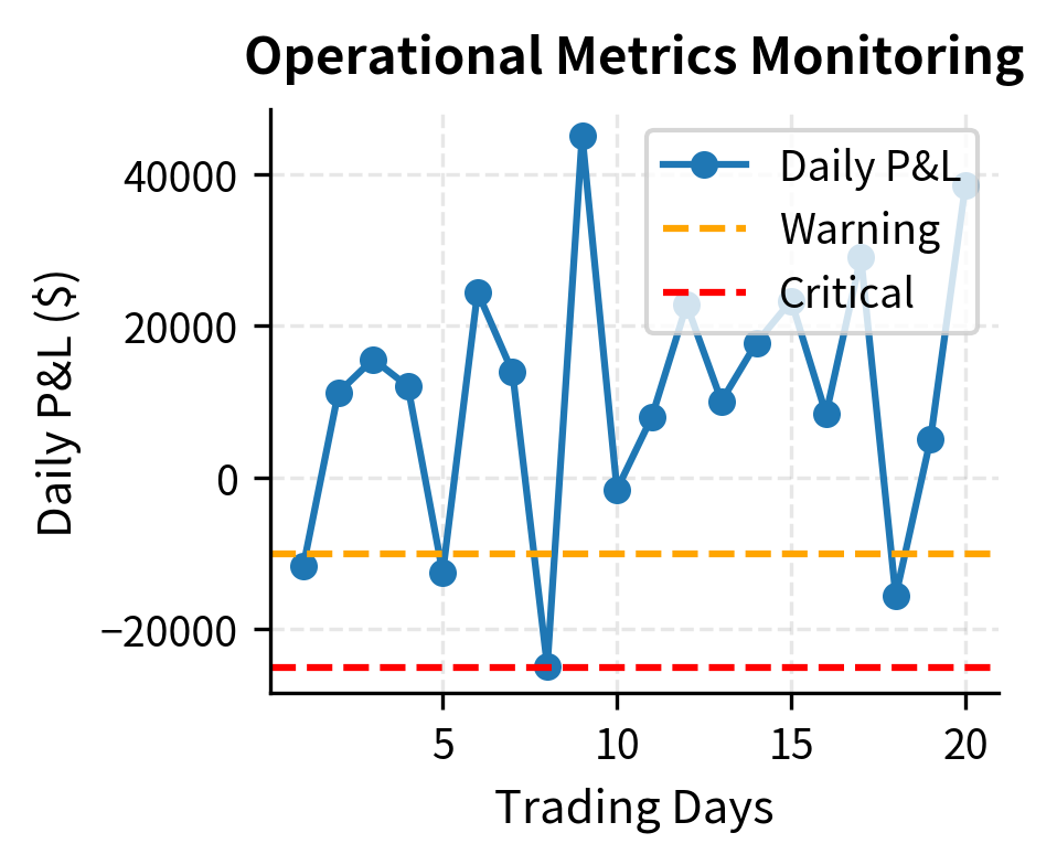
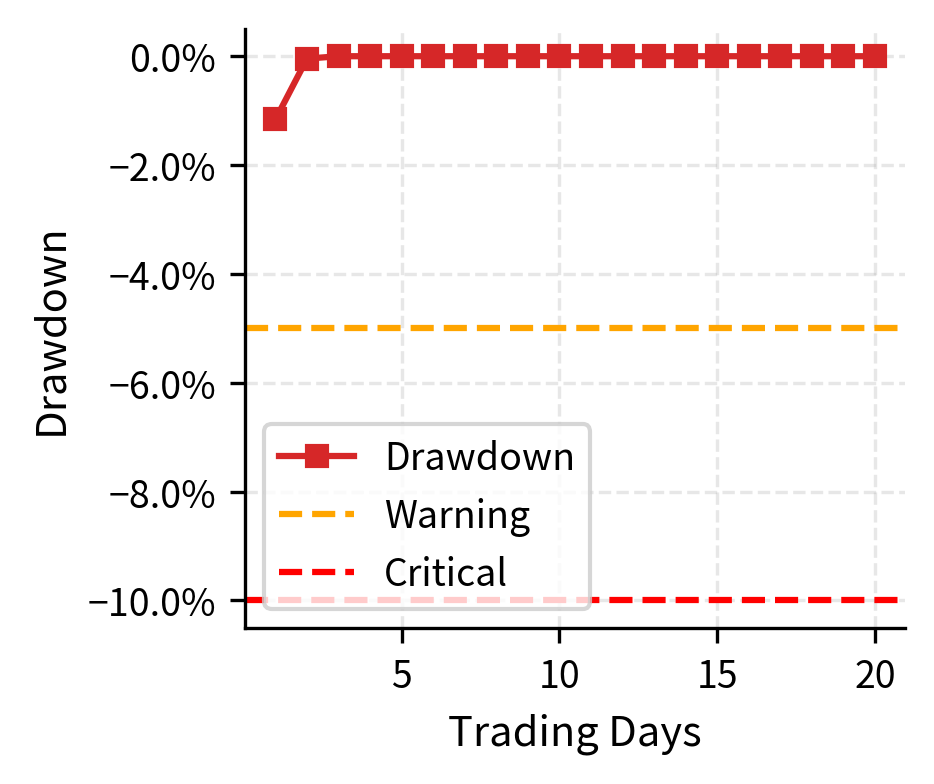
Effective monitoring strikes a balance between comprehensiveness and signal-to-noise ratio. You want to detect genuine problems quickly, but you also want to avoid alert fatigue that causes you to ignore warnings. The monitoring system below demonstrates this balance: it tracks multiple metrics continuously but only generates alerts when values cross defined thresholds. Different alert levels, from informational to critical, help prioritize response.
The dashboard aggregates critical health metrics, providing a snapshot of the strategy's operational status. The active alerts draw attention to the drawdown and Sharpe ratio degradation, ensuring that you can take corrective action before performance issues compound. In a production environment, these alerts would be routed to pagers, Slack channels, or other notification systems to ensure timely response.
Risk Controls and Circuit Breakers
Automated risk controls prevent catastrophic losses. Circuit breakers halt trading when predefined limits are breached, giving you time to assess the situation.
The philosophy behind risk controls is defense in depth. No single control is perfect, so multiple overlapping controls provide redundancy:
- Position Limits: Prevent concentration in a single stock.
- Gross Exposure Limits: Prevent excessive leverage.
- Daily Loss Limits: Stop trading before a bad day becomes a catastrophic day.
Each control addresses a different failure mode, and together they create a robust safety system.
The risk controller enforces safety boundaries by vetting every order against pre-configured limits. The results show how the system handles different violations: approving compliant orders, reducing those that hit soft limits, and blocking those that breach hard limits, thereby acting as a crucial safeguard against algorithmic errors. The soft limit mechanism is particularly valuable because it allows trading to continue at a reduced scale rather than stopping completely, maintaining some exposure while limiting risk.
Risk Control Parameters
The risk control system relies on carefully chosen parameters that balance protection against the operational friction of excessive constraints. Each parameter represents a judgment about acceptable risk levels.
The daily_loss_limit parameter establishes the maximum acceptable loss for a single trading session. This limit exists because bad days happen: a strategy that loses money on average would have been caught in backtesting, but even profitable strategies experience losing days. The question is how much loss is acceptable before you stop and reassess. The hard limit triggers an automatic trading halt to prevent further damage. The soft limit generates warnings that allow for human judgment about whether to continue. Setting these limits requires balancing the cost of stopping trading (missing potential recovery) against the cost of continuing (potentially larger losses). A common approach is to set the hard limit at a level where you would definitely want to pause and investigate, and the soft limit at a level where you want to be aware but might choose to continue.
The position_limit parameter caps the size of any individual position. This ensures the portfolio remains diversified and limits idiosyncratic risk. A single stock that declines 20% should not devastate the portfolio. The appropriate limit depends on your investment universe and return expectations: a strategy that makes 0.5% per trade can afford smaller position limits than one that makes 5% per trade, because the expected return scales with position size but the diversification benefit does not.
The gross_exposure_limit parameter controls the maximum total value of long and short positions combined. This controls the overall leverage and market exposure of the strategy. A gross exposure of 200% of NAV (100% long and 100% short) exposes the strategy to significant market risk on both sides. Higher leverage amplifies both returns and losses, and beyond a certain point, the risk of margin calls during drawdowns becomes unacceptable.
The concentration_limit parameter sets the maximum percentage of the portfolio allocated to a single asset. This prevents the strategy from becoming overly dependent on the performance of one stock. Even when signals strongly favor a particular position, concentration limits ensure that errors in the signal or unexpected events affecting that stock cannot cause catastrophic losses. A 10% concentration limit means that even a complete loss on a single position caps the portfolio impact at 10%.
Continuous Evaluation and Strategy Lifecycle
Deploying a strategy is not the end of the journey. Markets evolve, and edges decay. Continuous evaluation determines whether a strategy should continue running, needs recalibration, or should be retired.
Detecting Performance Degradation
Statistical tests help distinguish between normal variance and genuine performance decay. The challenge is detecting problems early without overreacting to noise.
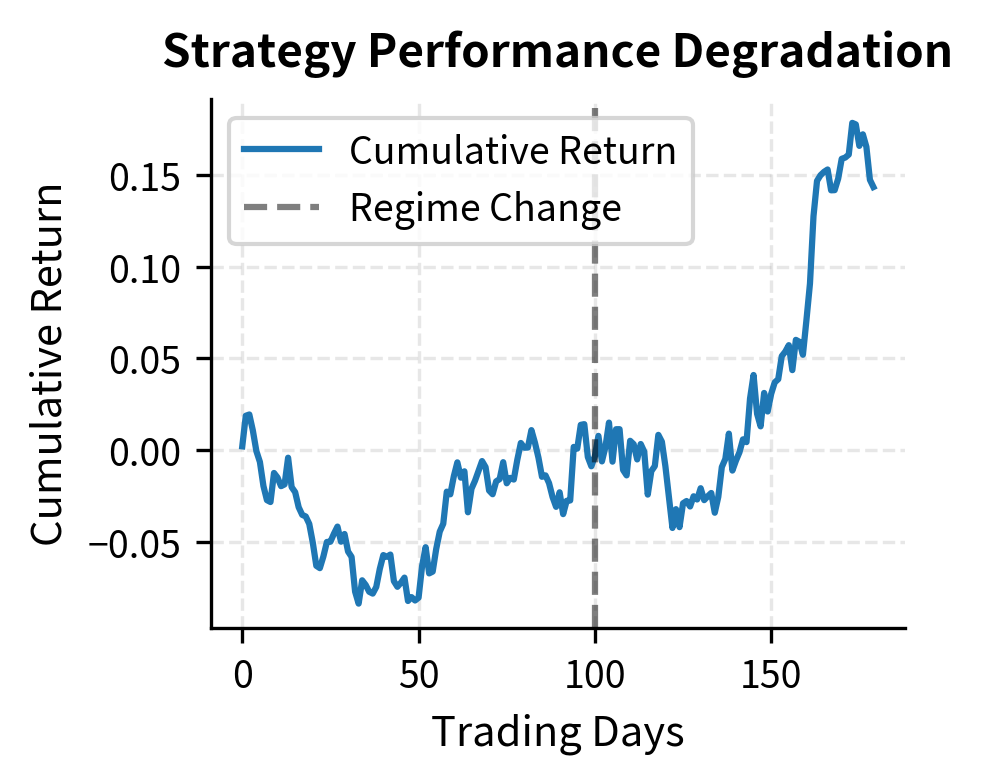
The fundamental difficulty in performance evaluation is distinguishing signal from noise. A strategy with a 1.0 Sharpe ratio will have many months where it appears to have a much lower Sharpe. This is not degradation; it is the nature of random returns. True degradation occurs when the underlying edge has diminished, but we observe only the noisy realized returns. Statistical tests help by quantifying how unlikely the observed returns would be if the strategy were performing at its historical level.
The performance evaluation identifies a statistical break in the strategy's returns. The degradation test flags the recent underperformance as significant, while the stability test confirms a shift in the underlying return distribution, providing objective evidence that the strategy may need recalibration or retirement. The combination of these tests provides stronger evidence than either alone: poor recent performance could be bad luck, but poor performance combined with a detected regime shift suggests a genuine change in strategy effectiveness.
Evaluation Parameters
The performance evaluation system depends on parameters that control the sensitivity and reliability of degradation detection.
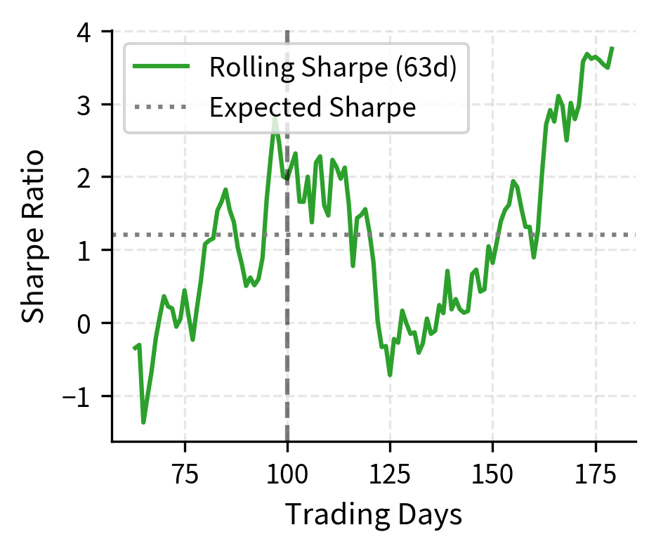
The window parameter sets the lookback period, such as 63 days, for calculating rolling metrics. This window determines the granularity of performance assessment. Shorter windows are more sensitive to recent changes but noisier, potentially generating false alarms from normal variance. Longer windows provide more stable estimates but may delay detection of genuine problems. A 63-day window, representing approximately one quarter, balances these considerations for most strategies. Strategies with higher expected Sharpe ratios can use shorter windows because their signal-to-noise ratio is better.
The confidence parameter establishes the statistical confidence level, such as 0.95, for the degradation test. This controls the false positive rate: a 95% confidence level means that we expect to incorrectly flag acceptable performance as degraded about 5% of the time. Higher confidence levels reduce false alarms but may delay detection of real issues. The appropriate level depends on the cost of each type of error. If stopping a profitable strategy is very costly, use higher confidence. If continuing a broken strategy is very costly, use lower confidence.
The expected_return parameter provides the baseline annualized return expected from the strategy. This serves as the null hypothesis for degradation testing: we ask whether observed returns are significantly below this level. Setting this parameter requires judgment about what the strategy should achieve. Too optimistic an expectation leads to frequent false alarms; too pessimistic an expectation lets genuine problems go undetected. The best approach is to use the return observed during out-of-sample testing before production, which provides a realistic benchmark free from in-sample optimization bias.
Strategy Lifecycle Management
Strategies have a natural lifecycle. They are born from research, mature through paper trading, live in production, and eventually retire as their edge decays. Managing this lifecycle systematically prevents the common mistake of running strategies long past their useful life.
The lifecycle framework below formalizes this process. Each strategy exists in exactly one state at any time, and transitions between states follow defined rules based on performance metrics. This structure ensures that decision-making about strategies is consistent and documented, avoiding the ad-hoc judgments that often keep underperforming strategies running too long or retire profitable strategies prematurely.
The lifecycle management system enforces a disciplined process for handling strategy evolution. By automatically transitioning the strategy to "Under Review" based on performance triggers, it ensures that deteriorating strategies are paused and assessed rather than being allowed to decay unnoticed in production. The state history provides an audit trail that documents why each transition occurred, which is valuable for learning from both successes and failures.
Limitations and Practical Considerations
The research pipeline and deployment processes described in this chapter provide a framework, but real-world implementation faces several challenges that merit careful consideration.
The gap between backtest and live performance remains the most persistent challenge in quantitative trading. Despite paper trading, some issues only manifest with real capital at stake. Market impact, adverse selection (where your fills are worse than average because informed traders are on the other side), and changes in market microstructure can all degrade performance. The transaction cost models from Chapter 2 help, but they are estimates. Production experience consistently shows that actual costs exceed model predictions, particularly for strategies that trade frequently or in less liquid instruments.
Experiment tracking and version control, while essential, can become burdensome bureaucracy if implemented without pragmatism. The goal is reproducibility and learning, not perfect documentation of every research dead end. You must find the right balance between tracking discipline and research velocity. Similarly, alerting systems require careful calibration. Too many false alarms cause alert fatigue, while too few miss genuine problems. The thresholds presented here are starting points that require tuning based on each strategy's characteristics.
The statistical tests for performance degradation carry their own limitations. Financial returns are not normally distributed, exhibit autocorrelation, and exist in a non-stationary environment. A t-test that assumes normality may give misleading p-values. More robust approaches use bootstrap methods or Bayesian inference, but even these struggle with the fundamental problem of small samples and changing market regimes. When a strategy underperforms for three months, distinguishing bad luck from genuine edge decay requires judgment that cannot be fully automated.
Production systems fail in unexpected ways. Network partitions, exchange outages, data feed errors, and software bugs all occur. The monitoring and alerting infrastructure described here catches many issues, but the most dangerous failures are often the silent ones, such as a strategy that continues to run but makes subtly wrong decisions due to stale data or a configuration error. Regular reconciliation against external sources and your review of trading activity remain essential complements to automated monitoring.
Summary
This chapter covered the complete lifecycle of a quantitative trading strategy, from initial hypothesis through production deployment and ongoing evaluation.
The key components of a robust research pipeline include disciplined hypothesis formulation, careful data quality control, systematic feature engineering, and structured iteration with experiment tracking.
Version control with Git manages code changes, while experiment tracking tools like MLflow capture the full context of each research run, enabling reproducibility and systematic comparison across experiments.
Paper trading bridges backtesting and live trading, revealing issues with data feeds, execution timing, and system reliability that historical simulations cannot detect. Strategies should pass paper trading validation criteria before receiving real capital.
Production deployment requires scheduling, monitoring, alerting, and automated risk controls. Circuit breakers halt trading when predefined limits are breached, providing time for human assessment.
Continuous evaluation using statistical tests helps detect performance degradation, though these tests have limitations given the non-stationarity of financial markets. Strategy lifecycle management provides a framework for transitioning strategies through research, production, and eventual retirement.
The next chapter on position sizing and leverage management builds on these deployment concepts by examining how to determine appropriate capital allocation across strategies and instruments.
Quiz
Ready to test your understanding? Take this quick quiz to reinforce what you've learned about the research pipeline and strategy deployment.

Comments