

Master execution algorithms from TWAP and VWAP to Almgren-Chriss optimal trading. Learn to balance market impact against timing risk for superior results.
Choose your expertise level to adjust how many terms are explained. Beginners see more tooltips, experts see fewer to maintain reading flow. Hover over underlined terms for instant definitions.
Execution Algorithms and Optimal Execution
When a portfolio manager decides to buy one million shares of a stock, the real challenge has just begun. Executing that order is not simply a matter of sending it to an exchange. As we explored in the previous chapter on market microstructure and as we examined in depth in our discussion of transaction costs and market impact, your large orders move markets. The very act of buying pushes prices higher, eroding the alpha that motivated the trade in the first place.
Execution algorithms emerged to solve this fundamental problem. Unlike the alpha-seeking strategies we covered in Part VI, execution algorithms have a different objective. They take a given trading decision as input and focus purely on minimizing the cost of implementation. A portfolio manager might use machine learning to identify an undervalued stock, but the execution algorithm's job is to buy that stock as cheaply as possible, not to question whether it should be bought at all. develops the theory and practice of optimal execution. We begin with simple schedule-based algorithms like TWAP and VWAP, progress to implementation shortfall frameworks, and culminate in the Almgren-Chriss model, which provides a rigorous mathematical foundation for balancing the competing costs that execution traders face. Understanding these algorithms is essential for anyone building or evaluating quantitative trading systems, as execution quality often determines whether a profitable strategy remains profitable after accounting for real-world frictions.
The Execution Problem
Consider an institutional trader who needs to sell 500,000 shares of a stock that trades approximately 2 million shares per day. Selling the entire position immediately would require crossing roughly 25% of the daily volume in a single burst, almost certainly moving the price against you and resulting in poor execution.
The alternative is for you to spread the execution over time, but this introduces a new risk. The price might move unfavorably while you wait. This tension between market impact and timing risk lies at the heart of optimal execution.
::: {.callout-note title="Market Impact vs. Timing Risk"} Market impact is the adverse price movement caused by your trading activity. Timing risk (also called price risk or volatility risk) is the risk that the asset price moves unfavorably while waiting to complete execution. Aggressive execution minimizes timing risk but maximizes impact, while patient execution minimizes impact but maximizes timing risk.
Understanding why this fundamental tension exists requires us to think carefully about the mechanics of trading. When a trader submits a large buy order, the immediate effect is to consume available liquidity on the ask side of the order book. As the order depletes offers at the best price, subsequent fills occur at increasingly worse prices. This is market impact in its most direct form. The trader's own activity causes the execution price to deteriorate. The more aggressively the trader buys, the more liquidity is consumed in a short window, and the more severe the impact.
Conversely, if the trader waits patiently, spreading the order over hours or even days, each individual trade is small enough to have minimal impact. However, during this extended waiting period, the underlying price is free to move based on market forces entirely unrelated to the trader's activity. Perhaps unfavorable news arrives, or the broader market sells off, or other participants independently decide to sell the same stock. This is timing risk, the random price movement that accumulates while the trader waits to complete execution.
Let's formalize the execution problem mathematically. You need to execute a position of shares over a time horizon . At any time , let denote the remaining inventory. The execution schedule specifies the trading rate , which represents how quickly shares are being executed at each moment. The negative sign appears because inventory decreases as trading proceeds. This trading rate must satisfy the fundamental constraint that execution completes by the horizon:
where:
- : trading rate at time measured in shares per unit time
- : execution time horizon
- : total shares to be executed
This integral constraint simply states that the cumulative amount traded over all time must equal the total order size. It ensures that the trader neither under-executes, leaving inventory unfinished, nor over-executes, trading beyond the intended position.
The trader's objective is to choose the trajectory that minimizes some cost function, typically involving both expected execution cost and its variance. The expected cost captures the average amount paid above the initial price, while the variance captures the uncertainty around that average. Different algorithms embody different trade-offs between these objectives, and different traders may prefer different points along the efficiency frontier depending on their risk tolerance and urgency.
Schedule-Based Algorithms
Schedule-based algorithms follow predetermined trading patterns, executing orders according to fixed rules regardless of short-term market conditions. These algorithms are simple, transparent, and widely used for benchmarking purposes.
Time-Weighted Average Price (TWAP)
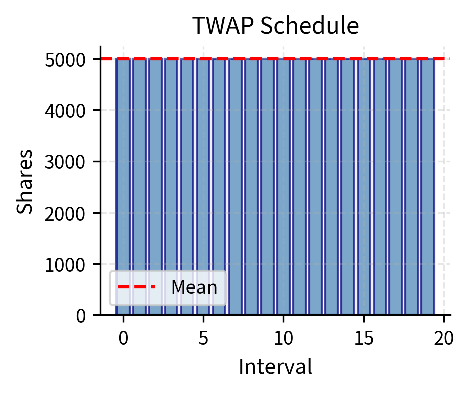
The simplest execution algorithm is TWAP, which divides the total order into equal-sized pieces and executes one piece at regular intervals throughout the trading period. The logic behind TWAP is straightforward: without any information about when liquidity will be available or when prices might be favorable, the most sensible approach for you is to spread risk evenly across time.
For an order of shares executed over intervals of duration , TWAP trades at a constant rate. In continuous time, this rate is simply the total shares divided by the total duration:
where:
- : trading rate in shares per unit time
- : total order size
- : total duration
This formula expresses a fundamental principle: TWAP commits to a fixed pace of execution that does not vary regardless of market activity. Whether the market is quiet or hectic, or whether spreads are narrow or wide, the algorithm continues trading at the same steady rate.
Equivalently, in discrete intervals where the trading day is divided into equal periods:
where:
- : shares traded in interval
- : total order size
- : number of intervals
Each interval receives exactly the same allocation of shares. The index ranges from 1 to , and every interval is treated identically regardless of its position in the sequence or the market conditions prevailing at that time.
TWAP's appeal lies in its simplicity: it requires no forecasting of volume patterns, no estimation of market impact parameters, and no optimization. You can implement TWAP with nothing more than a clock and a calculator. The algorithm performs well when true trading costs are linear in execution rate and when the trader has no information about intraday volume patterns. In such circumstances, there is no basis for preferring one time period over another; equal treatment of all periods is the natural choice.
The output confirms that the algorithm divides the total order into equal chunks, ensuring a constant trading rate regardless of market activity or price movements.
Volume-Weighted Average Price (VWAP)
VWAP improves on TWAP by executing in proportion to expected market volume. The key insight motivating VWAP is that markets naturally absorb more trading during high-volume periods, so concentrating execution during these times reduces market impact. Think of it this way. If one million shares trade during the open but only one hundred thousand during lunch, submitting your large order during the open will constitute a smaller fraction of total activity and therefore have less price impact.
If represents the expected volume in interval and is total expected volume across all intervals, then VWAP allocates shares according to the volume weights:
where:
- : target shares to trade in interval
- : total order size
- : expected volume in interval
- : total expected volume
This formula ensures that the algorithm participates at a consistent rate relative to market activity. When volume is high, the algorithm trades more shares. When volume is low, the algorithm trades fewer shares. The ratio represents the fraction of daily volume expected in interval , and this same fraction is applied to the total order size.
The VWAP benchmark itself, which gives the algorithm its name, is defined as the volume-weighted average of all prices observed during the trading period:
where:
- : volume-weighted average price benchmark
- : price in interval
- : volume in interval
- : total number of intervals
This benchmark represents the average price at which all market participants traded during the period, with more weight given to prices during high-volume intervals. A VWAP algorithm aims to achieve an average execution price close to this benchmark. If the algorithm executes exactly according to the volume profile, it will by construction achieve a price equal to the market VWAP, assuming prices don't move in response to the algorithm's own trading.
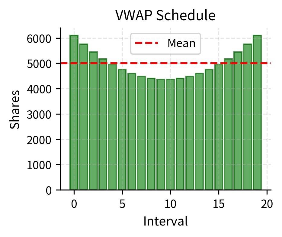
The figure illustrates a key difference between the two approaches. TWAP maintains constant execution throughout the day, while VWAP front-loads and back-loads execution to match the typical U-shaped volume pattern observed in equity markets.
Limitations of Schedule-Based Algorithms
While simple and transparent, schedule-based algorithms have significant limitations:
- No adaptation to conditions: They execute regardless of whether the spread is wide, the order book is thin, or prices are moving adversely
- Predictability: Sophisticated market participants can detect and exploit predictable execution patterns
- Benchmark mismatch: Matching a volume-weighted benchmark may not align with minimizing actual execution cost
TWAP performs poorly when volume varies significantly throughout the day, while VWAP can underperform when the actual volume distribution differs from the historical pattern used for scheduling. Both approaches ignore the trader's risk preferences and the specific characteristics of the security being traded.
Implementation Shortfall
Implementation shortfall, introduced by André Perold in 1988, measures the total cost of implementing an investment decision. Unlike TWAP or VWAP, which compare execution to market-derived benchmarks, implementation shortfall compares your actual performance to a "paper portfolio" that could have been achieved if your entire trade executed instantaneously at the decision price.
Implementation shortfall is the difference between the theoretical return of a paper portfolio, executed at decision prices with no costs, and the actual return of the real portfolio, executed over time with market impact and other costs. It captures the full cost of translating investment ideas into actual positions.
The power of implementation shortfall as a concept lies in its comprehensiveness. When you identify an opportunity, say a stock trading at $50 that you believe is worth $60, the value of that idea is based on the price at which the decision was made. Every penny your actual execution price deviates from that decision price represents value lost, value that transfers from your trading strategy to the market or to intermediaries. Implementation shortfall captures all of these costs in a single unified measure.
Components of Implementation Shortfall
Implementation shortfall can be decomposed into several components that help identify where execution costs originate. Let be the decision price (the price when the trading decision was made), the average execution price achieved across all fills, and the price at the end of the trading period.
For a buy order of shares, the total implementation shortfall is simply the difference between what was paid and what would have been paid at the decision price:
where:
- : total shares
- : average execution price
- : decision price
This total shortfall represents the aggregate cost of execution, but it does not reveal where those costs came from. To gain deeper insight, we can decompose the shortfall into components that isolate different sources of slippage:
where:
- : implementation shortfall
- : total shares
- : average execution price
- : decision price
- : benchmark price representing value absent trading (e.g., VWAP or arrival price)
The market impact component captures the portion of the price movement that can be attributed to the trader's own activity. The timing cost component captures price drift that would have occurred even without the trader's participation, reflecting market movements that happened simply because execution took time.
A more detailed decomposition, often used in transaction cost analysis, includes additional components:
- Delay cost: Price movement between decision and start of execution, capturing the cost of any lag between deciding to trade and entering the market
- Market impact cost: Adverse price movement caused by our trading, the direct consequence of consuming liquidity
- Timing cost: Unfavorable price drift during execution, representing exposure to random market movements
- Opportunity cost: Cost of any unexecuted portion, relevant when the algorithm fails to complete the full order
Implementation Shortfall Algorithms
Implementation shortfall (IS) algorithms attempt to minimize expected shortfall while controlling its variance. Unlike VWAP, which targets a benchmark regardless of market conditions, IS algorithms adapt their aggressiveness based on an urgency parameter specified by you. The urgency parameter controls the trade-off between market impact and timing risk, allowing you to express your preferences about how to balance these competing concerns. High urgency means execute quickly to minimize timing risk while accepting higher market impact. Low urgency means execute patiently to minimize impact, accepting higher timing risk.
If you believe prices are about to move unfavorably or if you have limited risk budget for the position, you would choose high urgency. If you have a long-term view and tolerance for volatility, you would choose low urgency, preserving capital by avoiding unnecessary impact costs.
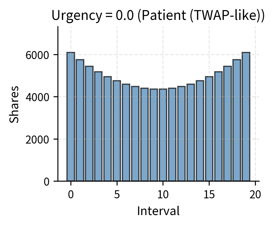
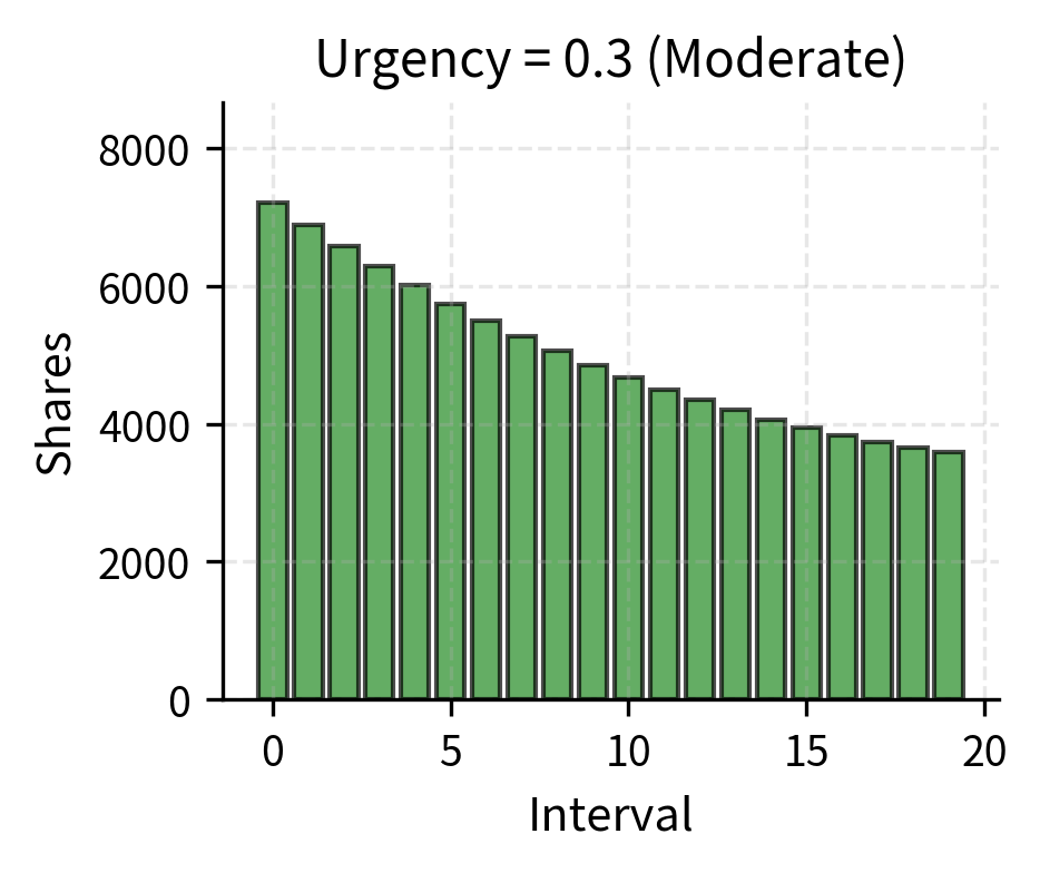
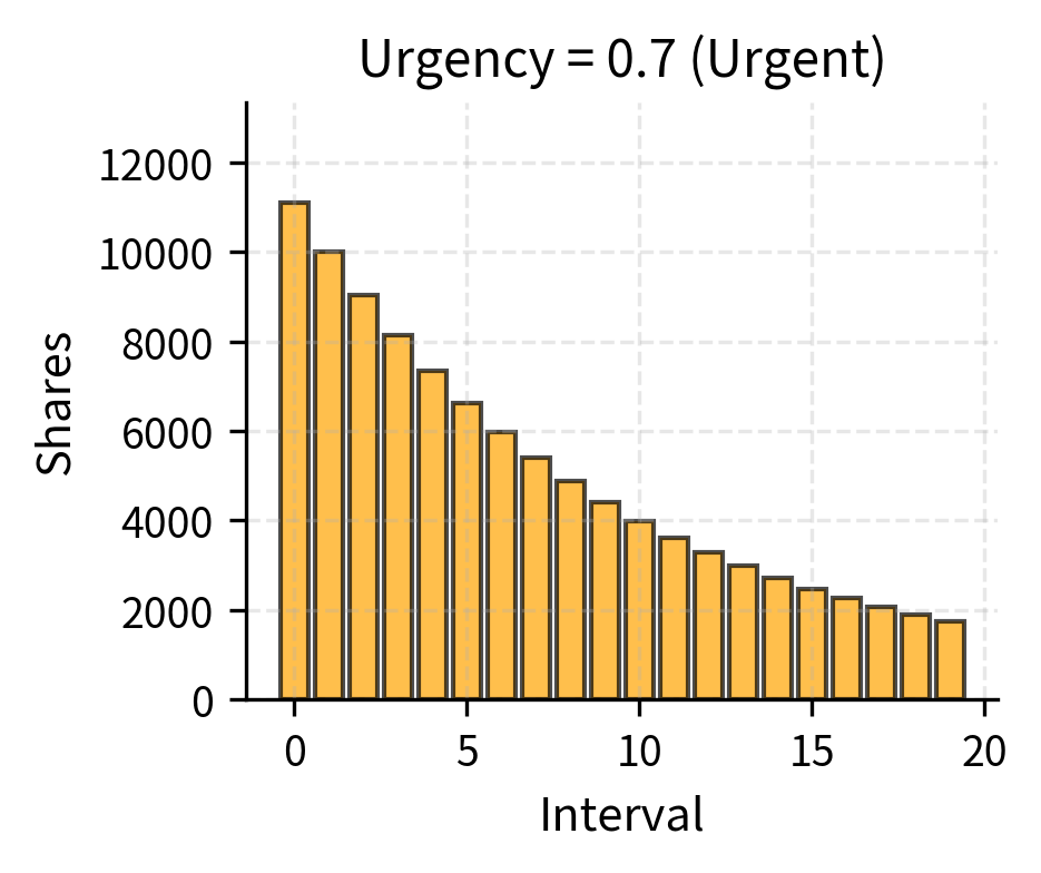
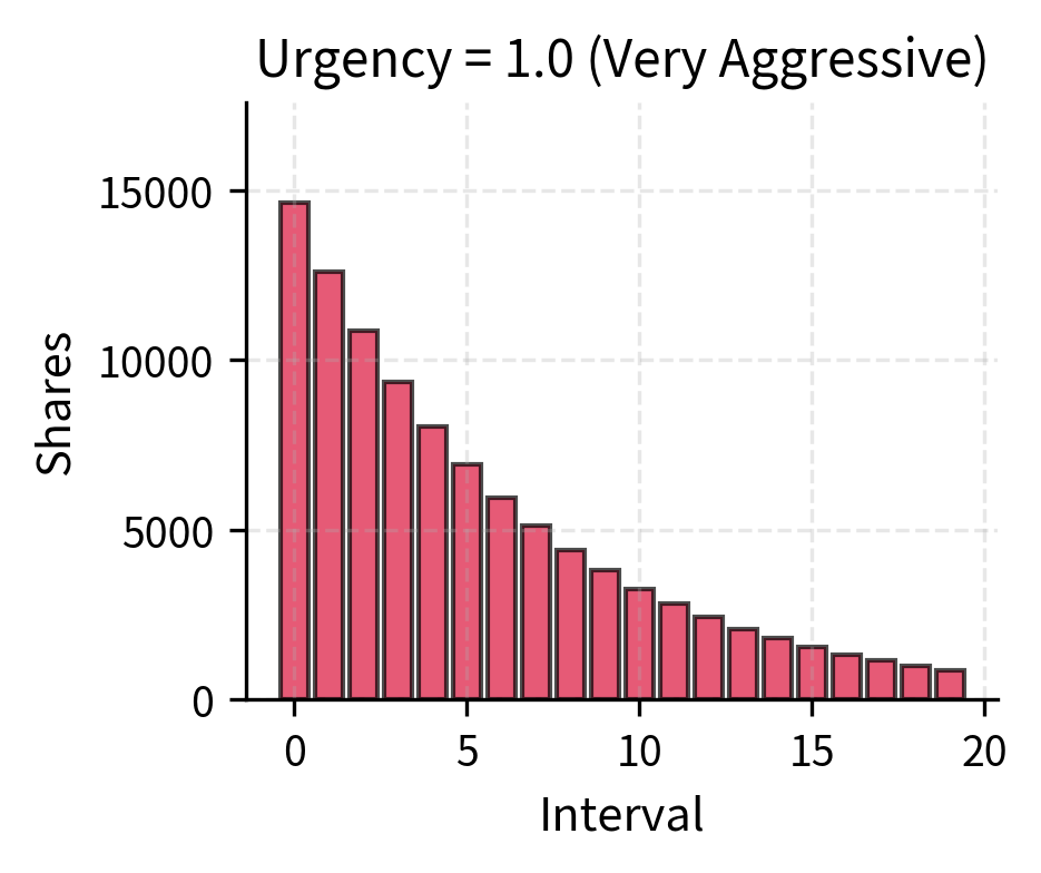
The visualization demonstrates how urgency transforms the execution profile. At zero urgency (0.0), the algorithm resembles VWAP. As urgency increases to 1.0, execution concentrates increasingly in early intervals, allowing traders to reduce price volatility exposure.
The Almgren-Chriss Framework
The Almgren-Chriss model, published in 2000, provides a rigorous mathematical framework for optimal execution. It formalizes the trade-off between market impact and timing risk, deriving closed-form optimal trajectories under specific assumptions about price dynamics and market impact. This framework provided explicit mathematical solutions that practitioners could implement and analyze.
Model Setup
The framework begins by modeling the midpoint price as following arithmetic Brownian motion. This means the price evolves randomly over time, with increments that are normally distributed and independent across time periods:
where:
- : midpoint price at time
- : arithmetic volatility, representing the standard deviation of price changes per unit time
- : standard Wiener process, the mathematical representation of random price fluctuations
Note the deliberate absence of drift in this equation. The framework assumes no alpha and no expected direction of price movement. This assumption is philosophically consistent with the role of execution. The decision about what to trade and why has already been made elsewhere; it is not the execution algorithm's responsibility. The execution algorithm's job is not to predict where prices are going but to minimize the cost of getting the desired position, given that prices will fluctuate randomly during execution.
You must liquidate shares over time horizon . Let denote remaining inventory at time , with initial condition (we start with the full position) and terminal condition (we must be completely liquidated by the horizon). The trading rate is , where the negative sign reflects that inventory decreases as we trade. A positive trading rate means we are selling, and our inventory is declining.
Market Impact Model
The model incorporates both temporary and permanent market impact, as we discussed in detail in the chapter on transaction costs. These two types of impact capture different mechanisms by which trading affects prices. When trading at rate :
- Permanent impact. A fraction of impact persists permanently, moving the midpoint price for all subsequent trades and the wider market. Permanent impact reflects the information content of order flow. When you trade, the market updates its beliefs about fair value. The cumulative permanent impact is , where is the permanent impact coefficient. Every share traded permanently shifts the price by in the adverse direction.
- Temporary impact. Additional adverse price movement affects only the current trade, not future ones. This Temporary impact reflects the cost of demanding immediacy. To trade quickly, one must pay for liquidity, crossing the spread or walking up the order book. The temporary impact is , where is the temporary impact coefficient measuring the additional cost per share from trading quickly, and represents fixed costs like half the bid-ask spread that must be paid regardless of trade size.
For mathematical tractability, and because the fixed cost does not affect the optimal trajectory shape, the model typically uses linear impact functions without the fixed component:
where:
- : permanent impact function describing how price permanently shifts with trading
- : temporary impact function describing additional cost for the current trade only
- : permanent impact coefficient in dollars per share per share traded
- : temporary impact coefficient in dollars per share per share traded
- : trading rate
The linearity assumption, while stylized, captures the essential economics. Trading faster costs more due to temporary impact, and total trading permanently moves prices. The distinction between temporary and permanent impact is crucial because permanent impact represents a cost that cannot be avoided by changing the trading schedule, while temporary impact depends critically on how aggressively we trade.
Expected Cost and Variance
The expected execution cost consists of permanent and temporary components. For a trading trajectory with trading rate , we can derive your expected cost by integrating the impact over time. The calculation proceeds as follows:
where:
- : expected execution cost across all trading
- : initial inventory to be liquidated
- : remaining inventory at time
- : trading rate at time
- : permanent impact coefficient
- : temporary impact coefficient
- : trading horizon
This derivation reveals a fundamental insight about the structure of execution costs. The expected cost decomposes into two qualitatively different terms. The permanent impact term depends only on total shares and is completely path-independent. No matter how we schedule our trades, we will pay this cost. The factor of one-half appears because early trades suffer the full permanent impact of later trades, while later trades have already "locked in" some of that impact, creating an averaging effect. The temporary impact term depends on the execution speed and is the only component we can minimize through clever scheduling. Because it is quadratic in the trading rate, this term penalizes bursts of rapid trading and rewards smooth, steady execution.
The variance of execution cost arises from the accumulation of price risk on the held inventory. The intuition is straightforward: while we hold shares, their value fluctuates randomly. The more shares we hold and the longer we hold them, the more exposed we are to these fluctuations. If the price evolves as , the fluctuation in portfolio value is . This stochastic integral represents the cumulative random gains and losses from price movements applied to our inventory over time.
By the Itô isometry, a fundamental result in stochastic calculus, the variance of this integral can be computed by integrating the squared integrand:
where:
- : variance of execution cost
- : price volatility per unit time
- : trading horizon
- : remaining inventory at time
This variance formula captures the essence of timing risk. The unexecuted inventory remains exposed to price volatility at every moment. The variance integrates because variance is a quadratic measure. Holding twice as many shares exposes us to four times the risk. An execution schedule that maintains high inventory for a long time will have high variance, while a schedule that rapidly reduces inventory will have low variance.
Mean-Variance Optimization
With expressions for both expected cost and variance in hand, we can formulate the optimization problem. The Almgren-Chriss objective balances expected cost against variance using a risk aversion parameter :
where:
- : execution trajectory over time, the decision variable we optimize
- : risk aversion parameter, expressing how much the trader dislikes variance relative to expected cost
This mean-variance formulation should feel familiar. It is directly analogous to Markowitz portfolio optimization, which we covered in Part IV. In portfolio theory, we balance expected return against portfolio variance when choosing asset weights. Here, instead of choosing portfolio weights, we choose an execution trajectory. Instead of maximizing return while controlling risk, we minimize cost while controlling execution uncertainty. The mathematical structure is identical, which is why the Almgren-Chriss framework produces an "efficient frontier" of execution strategies just as Markowitz produces an efficient frontier of portfolios.
The risk aversion parameter is chosen by the trader and reflects their preferences. A trader with high risk aversion, large , will pay more in expected impact to achieve certainty about execution cost. A trader with low risk aversion, small , will accept uncertain outcomes in exchange for lower expected cost. There is no objectively "correct" value for ; it depends on the trader's circumstances, constraints, and risk tolerance.
The Optimal Trajectory
To derive the optimal trajectory, we must solve this optimization problem using calculus of variations. We first observe that the permanent impact term depends only on total shares , not the trading path. Since this term is the same for all feasible execution schedules, we can drop it from the optimization without affecting which trajectory is optimal.
Substituting the trading rate into the remaining cost and variance terms gives the objective functional that we seek to minimize:
where:
- : objective functional to minimize, a function of the entire trajectory
- : temporary impact coefficient
- : time derivative of inventory, equal to negative of trading rate
- : risk aversion parameter
- : volatility parameter
- : inventory at time
The integrand acts as the Lagrangian . This Lagrangian has the structure of a harmonic oscillator in classical mechanics, with a term quadratic in position (inventory) and a term quadratic in velocity (trading rate). This connection to physics is not merely coincidental; the same mathematical structure appears whenever a system must balance a position penalty against a velocity penalty.
The Euler-Lagrange equation provides the necessary condition for optimality. Any trajectory that minimizes the functional must satisfy:
where:
- : Lagrangian function
- : state variable representing inventory
- : time derivative of state variable representing trading rate
Calculating the necessary partial derivatives from our Lagrangian:
where:
- : Lagrangian function
- : inventory at time
- : first time derivative of inventory (negative of trading rate)
- : second time derivative of inventory (negative of rate of change of trading rate)
- : risk aversion parameter
- : volatility parameter
- : temporary impact coefficient
Substituting these expressions into the Euler-Lagrange equation yields the governing linear differential equation:
where:
- : second time derivative of inventory
- : risk aversion parameter
- : price volatility
- : temporary impact coefficient
- : inventory at time
This is a second-order linear ordinary differential equation with constant coefficients. The positive coefficient on indicates that solutions will be hyperbolic functions rather than trigonometric ones. Solving this ODE subject to boundary conditions (we start with full inventory) and (we must be fully liquidated by the horizon) yields a remarkable result: the optimal trajectory has a closed-form solution expressible in terms of hyperbolic functions.
Defining the risk-adjusted time constant that emerges naturally from the coefficient ratio:
where:
- : decay constant for the optimal trajectory, with units of inverse time
- : risk aversion parameter
- : price variance rate
- : temporary impact coefficient
This parameter plays a central role in the solution. It combines all the relevant model parameters into a single quantity that determines the shape of optimal execution. The numerator represents the marginal cost of holding inventory, risk aversion times variance, while the denominator represents the marginal cost of trading faster. The ratio balances these competing costs, and the square root converts this ratio into a time-scale parameter.
The optimal inventory trajectory is:
where:
- : optimal remaining inventory at time
- : initial inventory
- : trading horizon
- : risk-adjusted decay constant
- : hyperbolic sine function, defined as
This elegant formula describes exactly how inventory should decline over time. The hyperbolic sine function ensures that the trajectory satisfies both boundary conditions. At , the argument is and the ratio equals 1, giving . At , the argument is 0 and , giving .
The optimal trading rate follows as the derivative of the inventory trajectory:
where:
- : optimal trading rate
- : initial inventory
- : risk-adjusted decay constant
- : trading horizon
- : time
- : hyperbolic cosine and sine functions, where
The trading rate is highest at the beginning when is largest, and decreases over time as the remaining horizon shrinks.
The parameter determines the shape of the optimal trajectory. It balances the marginal cost of slow execution (timing risk, proportional to λ σ 2) against the marginal cost of fast execution (temporary impact, proportional to η). When κ is large as with high risk aversion or volatility and low temporary impact, optimal execution is front-loaded. When is small, execution approaches TWAP.
The optimal trajectory encompasses several intuitive limiting cases that help build understanding of what the solution means:
-
Risk-neutral trader (λ → 0): When you have no risk aversion, κ → 0 and the optimal strategy approaches TWAP. Without concern for timing risk, there is no reason to accept higher impact by trading quickly. Mathematically, as , the ratio approaches , which is the linear inventory path of TWAP.
-
Infinite risk aversion (λ → ∞): When timing risk is completely unacceptable, κ → ∞ and you liquidate immediately, accepting maximum market impact. You effectively treat any exposure to price uncertainty as infinitely costly and are willing to pay any amount in impact to eliminate it.
-
High volatility: Increasing σ increases κ, leading to faster execution. Higher volatility means greater timing risk per unit time, which justifies the acceptance of more impact to complete sooner. This makes intuitive sense: if prices are whipping around wildly, you want to finish quickly rather than remain exposed.
-
High temporary impact: Increasing η decreases κ, leading to slower execution. When impact is costly, patience pays off, as each share of accelerated trading costs more. This captures the fundamental trade-off: when impact is cheap, trade fast; when impact is expensive, trade slow.
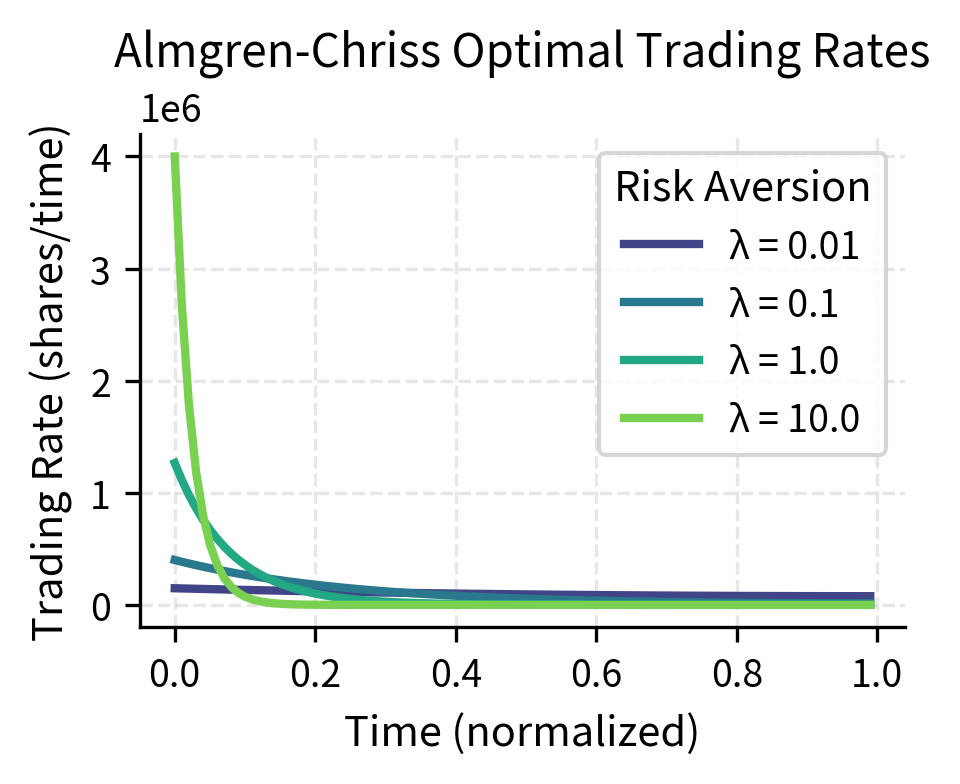
The trajectories reveal the fundamental insight of the Almgren-Chriss model. A risk-neutral trader () executes nearly linearly, resembling TWAP. As risk aversion increases, the trajectory becomes increasingly convex, with rapid early execution that slows as the position decreases. The most risk-averse trader () completes over half the execution in the first 20% of the time horizon.
Computing Expected Cost and Risk
The optimal trajectory achieves a specific expected cost and variance that depend on the model parameters. These expressions allow you to understand what you gain and give up by choosing a particular level of risk aversion. For the Almgren-Chriss solution:
where:
- : minimal expected cost achievable for the given risk aversion
- : permanent and temporary impact coefficients
- : risk-adjusted decay constant
- : total shares
- : time horizon
- : hyperbolic cosine and sine functions
The first term represents the unavoidable permanent impact cost that applies regardless of execution strategy. The second term represents the minimized temporary impact cost and depends on how aggressively we trade. A higher (more aggressive trading) increases this term because we incur more temporary impact.
The minimal variance of the execution cost is given by integrating the squared inventory trajectory:
where:
- : minimal cost variance for the given trajectory
- : price volatility
- : optimal inventory trajectory
- : trading horizon
This integral can be computed in closed form using properties of hyperbolic functions. The key observation is that faster execution, higher , reduces variance by reducing the integral of squared inventory but increases expected cost through higher temporary impact.
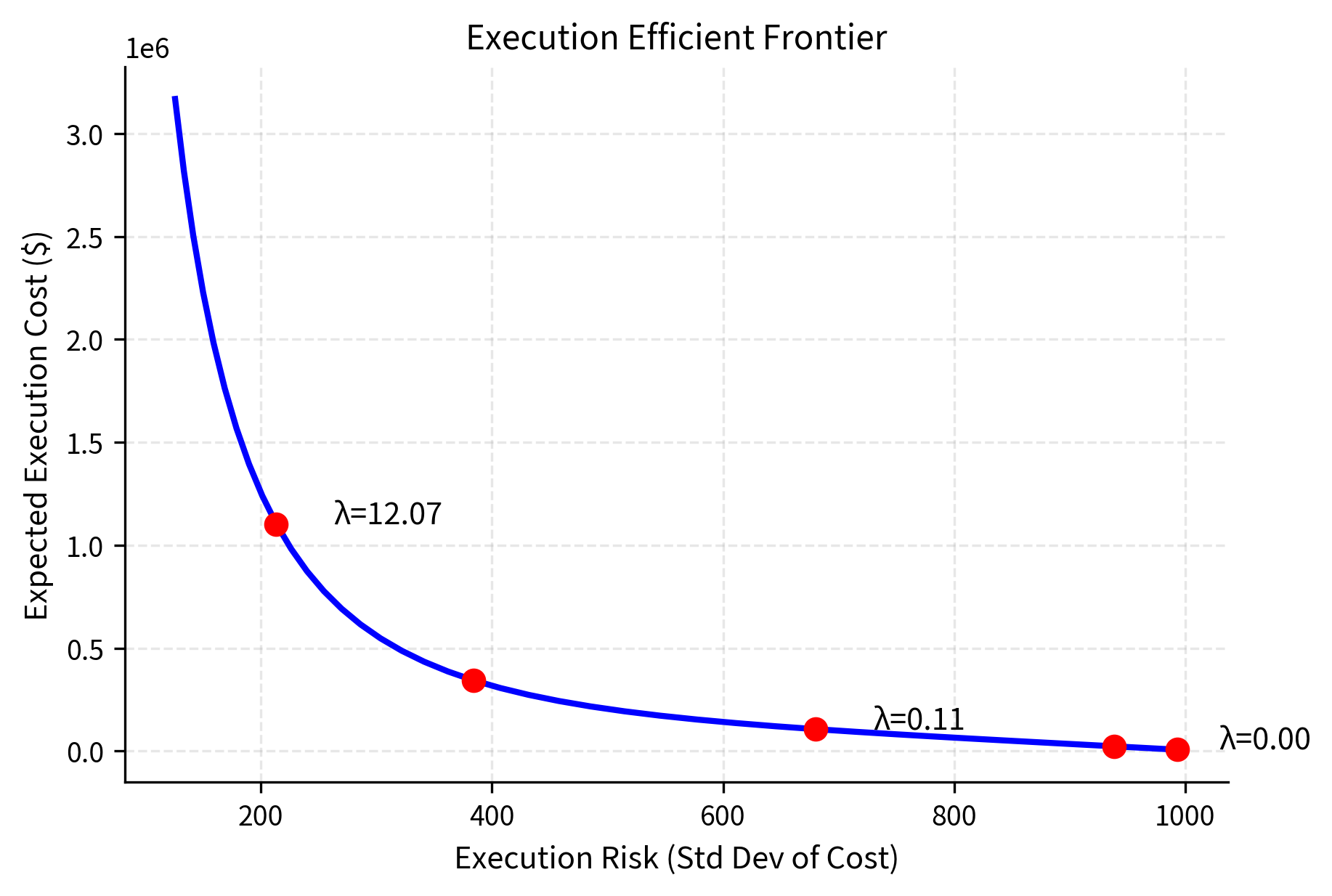
The efficient frontier illustrates that reducing execution risk requires accepting higher expected cost. Just as in portfolio theory, there is no free lunch: faster execution eliminates timing risk but increases market impact. The trader's risk aversion determines where on this frontier they should operate.
Adaptive Execution Algorithms
While the Almgren-Chriss framework provides optimal trajectories given known parameters, real markets present additional challenges. Volatility fluctuates, liquidity varies, and short-term price movements may signal information. Adaptive algorithms modify their behavior in response to market conditions.
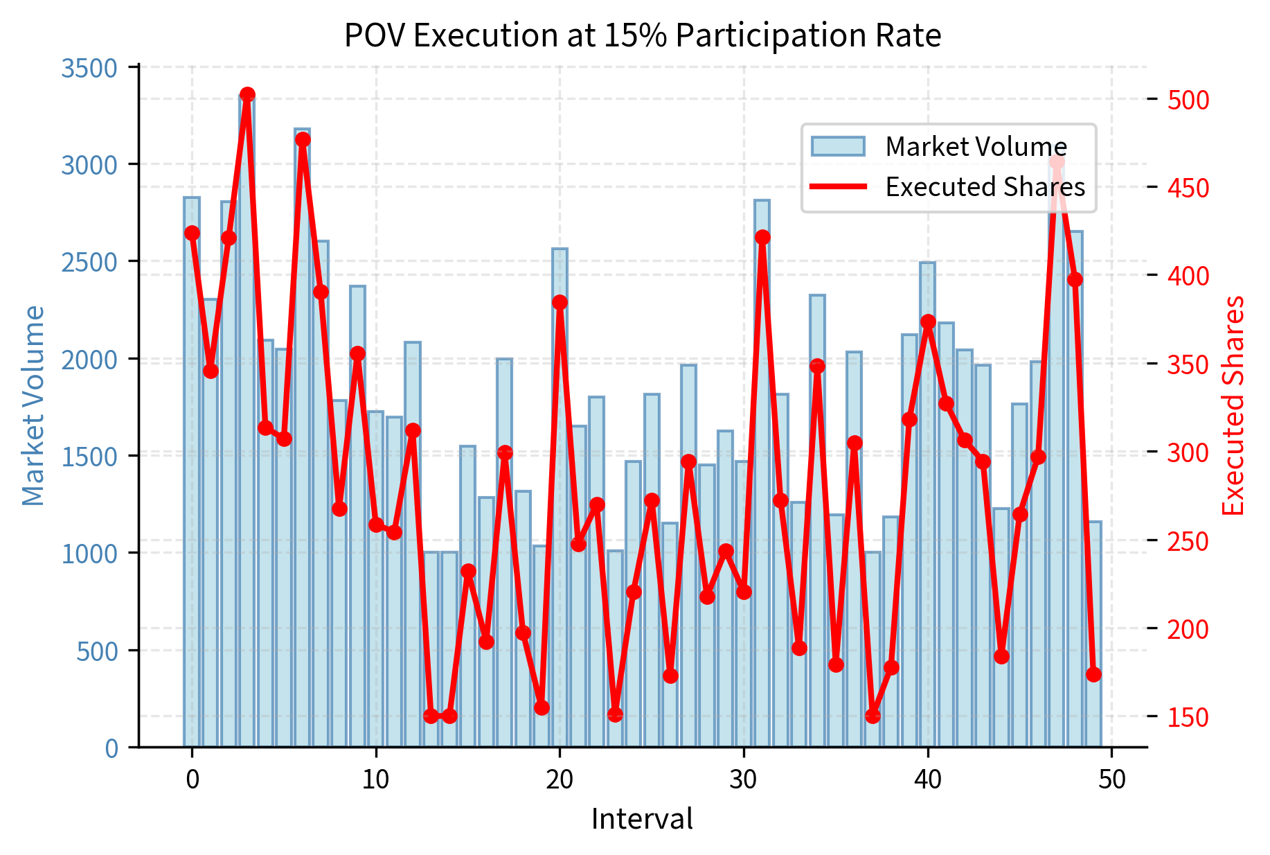
Percentage of Volume (POV)
Percentage of Volume algorithms trade as a fixed fraction of observed market volume, adapting execution speed to current liquidity. The algorithm monitors real-time trading activity and participates proportionally. This approach gives you natural camouflage.
where:
- : trading rate at time
- : target participation rate, typically between 5% and 20%
- : observed market volume at time
The participation rate is specified by you and represents what fraction of all market activity the algorithm should constitute. A 10% participation rate means that for every 100 shares traded in the market the algorithm trades 10.
POV offers natural camouflage. By trading proportionally with the market, your algorithm's activity is harder to distinguish from background flow. Other market participants cannot easily detect that your algorithmic execution is underway because the trading pattern mirrors overall market activity. POV also automatically slows during thin markets and accelerates during liquid periods, providing a built-in adaptation mechanism that schedule-based algorithms lack.
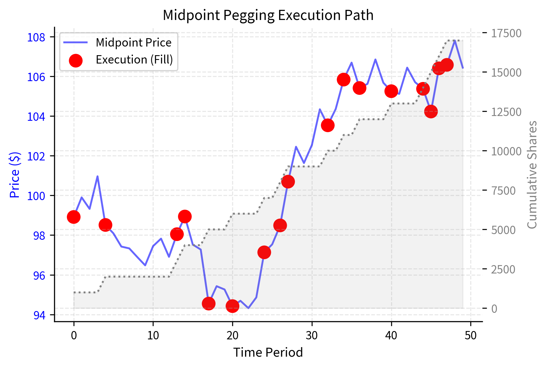
Pegging Algorithms
Pegging algorithms dynamically adjust limit order prices to maintain a position relative to the current market. Rather than crossing the spread to execute immediately, these algorithms post passive orders that capture Common peg types include:
- Midpoint peg: order price tracks the midpoint between bid and ask, offering price improvement to both sides
- Primary peg: order tracks the same-side best quote, joining the queue at the bid for buys or the ask for sells
- Passive peg: order tracks one tick behind the best quote for added price improvement at the cost of lower fill probability
These algorithms are useful when you prioritize execution price. By posting limit orders rather than crossing the spread, pegging algorithms capture the spread rather than paying it but risk non-execution if the market moves away.
Adaptive Shortfall Algorithms
Modern implementation shortfall algorithms combine the theoretical foundation of Almgren-Chriss with real-time adaptation. Rather than committing to a fixed trajectory computed at the start of execution, these algorithms continuously revise their plans based on incoming market data. Key features include:
- Intraday volatility estimation: adjusting urgency based on current versus expected volatility
- Spread monitoring: slowing execution when spreads widen beyond normal levels
- Momentum detection: accelerating or decelerating based on short-term price trends
- Volume surprise: adjusting participation when actual volume differs from forecast
These algorithms maintain a target trajectory as a baseline but allow deviations when market conditions diverge significantly from expectations.
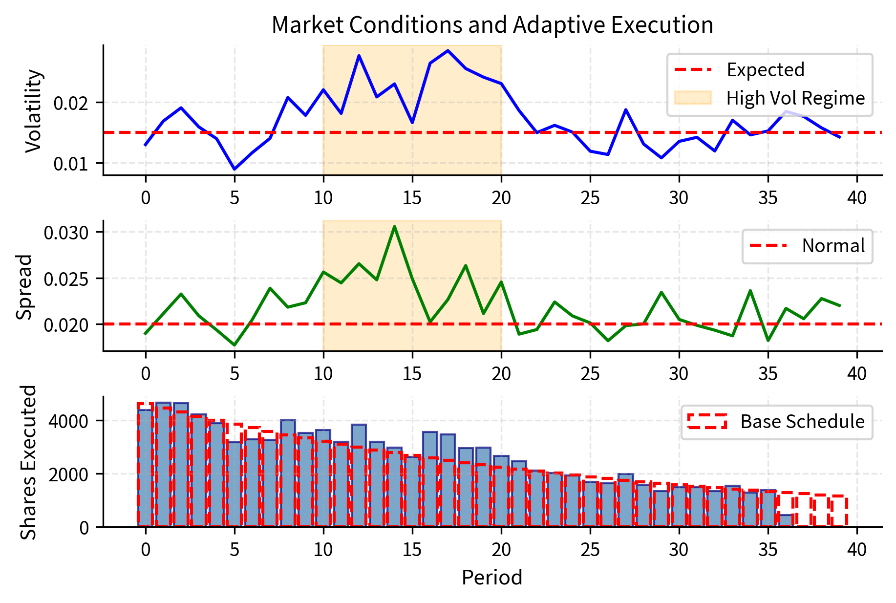
The adaptive algorithm increases execution during the high-volatility regime (periods 10-20) to reduce timing risk, while the widened spreads partially counteract this acceleration. This dynamic adjustment is impossible with static schedules like TWAP or pre-computed VWAP.
Putting It All Together: An Execution Simulator
To solidify these concepts, let's build a complete execution simulation that compares algorithm performance across different market scenarios.
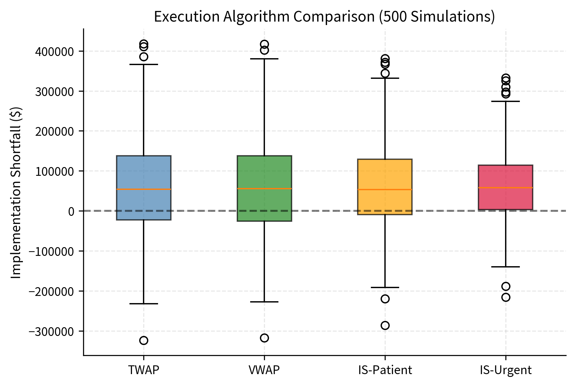
The simulation reveals the trade-offs inherent in execution algorithm selection. TWAP provides stable, predictable performance but misses opportunities to reduce timing risk. The urgent IS algorithm achieves the lowest average shortfall by completing execution quickly, but exhibits higher variance because it's more sensitive to the initial price movements. The "Sharpe-like" ratio (negative mean shortfall divided by standard deviation) provides a risk-adjusted measure of execution quality.
Limitations and Practical Considerations
The theoretical frameworks presented here provide valuable intuition, but practitioners must navigate several challenges when implementing execution algorithms in production.
Model Limitations
The Almgren-Chriss framework assumes linear market impact but empirical research consistently finds that impact is concave. Your first thousand shares have greater per-share price impact than your next thousand. Square-root impact models often fit data better:
where:
- : price impact
- : volatility
- : order size
- : market volume
However, these models do not yield closed-form optimal trajectories.
Similarly, the assumption of constant volatility fails during news events, earnings announcements, and market stress. Adaptive algorithms attempt to address this but accurate real-time volatility estimation remains challenging. The model also ignores the bid-ask spread and other fixed costs, which can dominate impact costs for smaller orders.
Parameter Estimation
Optimal execution requires knowing impact coefficients and , volatility , and risk aversion . Permanent impact is notoriously difficult to measure. It requires separating the price movement caused by your trading from the price movement that would have occurred anyway. Temporary impact estimates are sensitive to the measurement window. These parameters likely vary by security, time of day, market conditions and order size. A model calibrated on historical data may perform poorly when your trading conditions change.
Adversarial Considerations
In practice, execution algorithms operate in an adversarial environment. High-frequency traders can detect algorithmic patterns and trade against them in a practice known as "algo sniffing." TWAP's predictability makes it particularly vulnerable. Even sophisticated algorithms can be reverse-engineered if their behavior is sufficiently regular. This creates pressure toward randomization and adaptation that goes beyond what theory suggests.
Implementation Details
The difference between theoretical and realized performance often comes down to implementation details that academic models ignore. These include:
- Order routing decisions
- Exchange selection
- Handling of partial fills
- Behavior at the close
- Response to exchange outages As we will discuss in the next chapter on trading systems infrastructure, these engineering challenges can easily overwhelm your theoretical gains from optimal scheduling.
Summary
This chapter developed the theory and practice of optimal execution, a critical component of your quantitative trading system. We covered several key concepts and algorithms:
Schedule-based algorithms provide simple, transparent approaches to execution. TWAP divides orders evenly across time, while VWAP weights execution according to expected volume patterns. These algorithms are easy for you to implement and explain, but they cannot adapt to changing market conditions.
Implementation shortfall measures the total cost of implementing a trading decision by comparing actual execution to a paper portfolio that traded at decision prices. IS algorithms balance market impact against timing risk based on trader-specified urgency parameters.
The Almgren-Chriss framework formalizes optimal execution as a mean-variance optimization problem. The key insight is that the optimal trajectory depends on a single parameter that balances timing risk (proportional to ) against temporary impact (proportional to If you are risk-averse, you should front-load execution, while if you are risk-neutral, you should approach TWAP.
Adaptive algorithms extend these theoretical foundations by adjusting to real-time market conditions. POV algorithms trade proportionally with market volume, pegging algorithms capture spread by posting passive orders, and adaptive IS algorithms modify their baseline trajectory based on volatility and spread observations.
Your choice of execution algorithm depends on your objectives, the characteristics of the security, and current market conditions. No single algorithm dominates in all scenarios. Understanding the trade-offs between impact and timing risk, and having the infrastructure to implement appropriate algorithms, often determines whether your theoretical alpha translates into realized profits. chapter addresses the systems and infrastructure required to deploy these algorithms in production environments.
Quiz
Ready to test your understanding? Take this quick quiz to reinforce what you've learned about execution algorithms and optimal execution.

Comments