

Learn how to collect and process human preference data for RLHF. Covers pairwise comparisons, annotator guidelines, quality metrics, and interface design.

This article is part of the free-to-read Language AI Handbook
Human Preference Data
The alignment problem, as we discussed in the previous chapter, fundamentally comes down to a question of measurement: how do we capture what humans actually want from language models? Abstract concepts like helpfulness, harmlessness, and honesty resist simple formalization. You cannot write a loss function that directly optimizes for "be genuinely helpful without being sycophantic." Instead, we must collect empirical data about human preferences and use that data to guide model behavior.
Human preference data serves as the empirical foundation for alignment. Rather than trying to specify desired behavior through rules or heuristics, we collect examples of humans choosing between model outputs. These choices encode implicit knowledge about what makes a response good: whether it answers the question correctly, whether the tone is appropriate, whether it avoids harmful content. The power of this approach lies in its ability to capture nuanced preferences that resist explicit specification.
This chapter covers the practical machinery of preference data collection: how to design comparison interfaces, what makes a good preference dataset, how to write annotator guidelines that produce consistent judgments, and how to measure and maintain data quality. These decisions affect the entire alignment pipeline, shaping the reward models we will train and determining how our models behave.
Preference Collection Paradigms
Human preferences can be collected in several formats, each with different tradeoffs for scalability, reliability, and information density. The format we choose shapes not only the annotation process but also the mathematical models we can apply to learn from the data. We must consider both the cognitive demands on annotators and the statistical properties of the resulting data.
Pairwise Comparisons
The dominant paradigm in RLHF presents annotators with two model responses to the same prompt and asks which is better. This format has become the standard for preference collection because it addresses both human and mathematical needs.
From the annotator's perspective, pairwise comparisons reduce a complex quality judgment to its simplest possible form. Instead of asking "how good is this response?" we ask "which of these two responses is better?" This reframing has several advantages:
- Cognitive simplicity: Comparing two options is easier than rating on an absolute scale. The annotator need only decide which response they would rather receive, not quantify exactly how much better one is than the other.
- Calibration-free: Annotators don't need to agree on what "4 out of 5" means. When two annotators both prefer response A over response B, they have communicated the same information regardless of whether they would have assigned different numerical ratings.
- Direct modeling: The data format aligns naturally with the Bradley-Terry model we'll cover in the next chapter. This mathematical framework was specifically designed to learn underlying quality scores from pairwise comparisons.
A pairwise comparison looks like:
Prompt: "Explain photosynthesis to a 10-year-old."

Response A: "Photosynthesis is how plants make food! Plants have
special parts called chloroplasts that capture sunlight..."

Response B: "Photosynthesis is the biochemical process by which
photoautotrophs convert electromagnetic radiation..."

Which response is better? [A] [B] [Tie]
The annotator selects which response better satisfies the implicit quality criteria. Most preference datasets discard or minimize tie votes, as they provide less signal for training reward models. This reflects a key insight: the most valuable information comes from cases where annotators can make a clear distinction between options.
Likert Ratings
An alternative approach asks annotators to rate individual responses on a numerical scale (e.g., 1-5 or 1-7). This captures absolute quality judgments:
Response: "Photosynthesis is how plants make food using sunlight..."

Rate this response:
[1 - Very Poor] [2] [3 - Adequate] [4] [5 - Excellent]
Likert ratings provide more information per annotation, but they suffer from calibration issues. Different annotators interpret the scale differently, and even the same annotator may shift their standards over time. One annotator's "4" might correspond to another annotator's "3," making it difficult to aggregate ratings across annotators without careful normalization procedures.
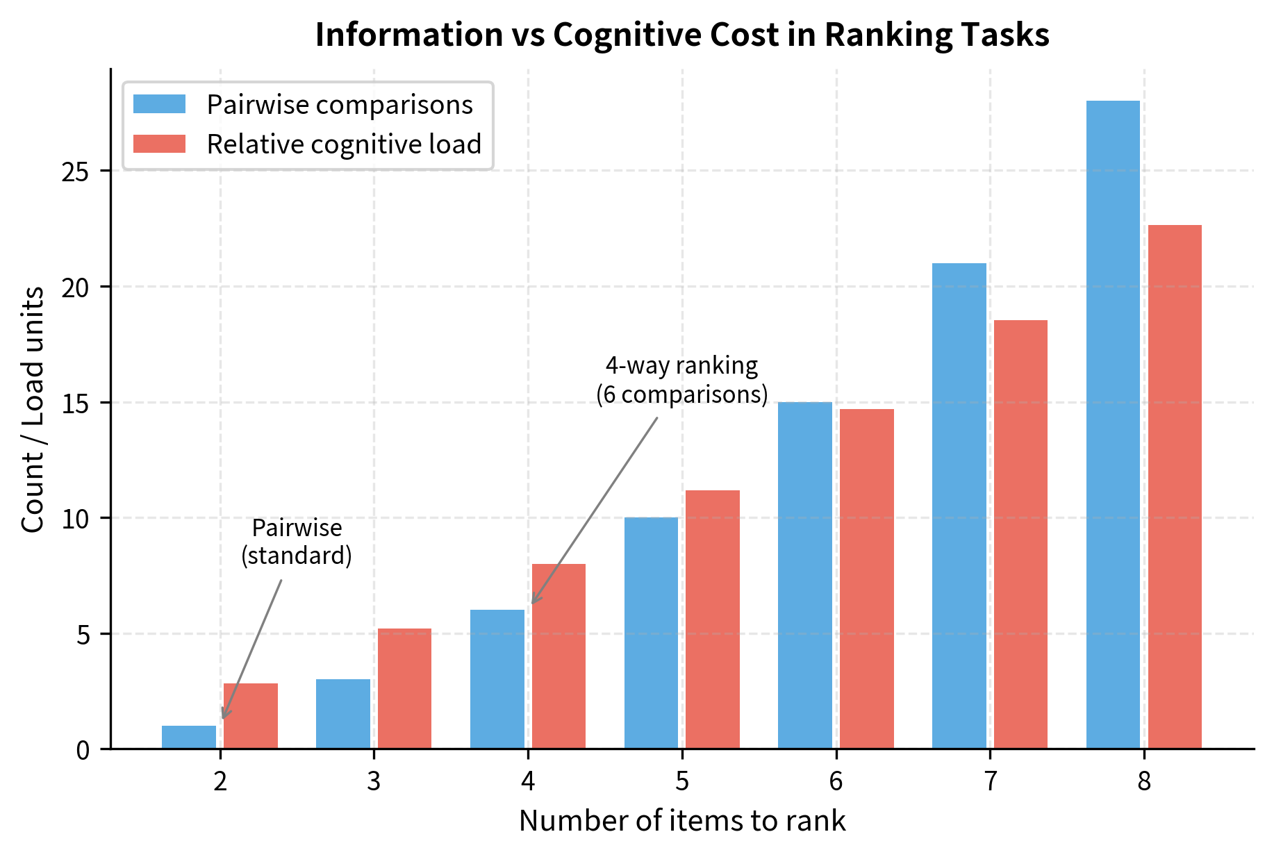
Ranking Multiple Responses
Some collection schemes present more than two responses and ask for a full ranking:
Rank these responses from best (1) to worst (4):

[ ] Response A
[ ] Response B
[ ] Response C
[ ] Response D
Rankings generate multiple pairwise comparisons from a single annotation task. Specifically, ranking 4 items yields 6 pairwise comparisons, since we learn the relative ordering of every pair. However, ranking becomes cognitively demanding as the number of items increases, and annotators may satisfice by only carefully distinguishing the top choices while making arbitrary decisions among lower-ranked items.
Why Pairwise Comparisons Dominate
Despite the information efficiency of rankings and the richness of ratings, pairwise comparisons remain the standard for several reasons. Understanding this choice illuminates important principles about preference data collection.
The first reason is reliability. Binary choices show higher inter-annotator agreement than multi-point scales. When forced to make a simple choice between two options, annotators tend to agree with each other more consistently than when asked to assign numerical scores. This higher agreement translates directly into cleaner training signal for reward models.
The second reason is theoretical grounding. The Bradley-Terry model provides a principled way to aggregate pairwise comparisons into reward scores. This model assumes that each response has some underlying "quality" and that the probability of preferring one response over another depends on the difference in their qualities. We will explore this model in depth in the next chapter, but the key point is that pairwise data fits naturally into this framework.
The third reason is practical simplicity. The interface is straightforward to build, the data format is simple to process, and the annotation task is easy to explain to new annotators. These practical considerations matter enormously when scaling to thousands of comparisons.
Most major preference datasets, including those used to train InstructGPT, Claude, and Llama 2, rely primarily on pairwise comparisons.
Collection Interface Design
The interface through which annotators provide preferences significantly impacts data quality. Small design decisions can introduce systematic biases or reduce annotator efficiency. A well-designed interface makes the annotator's job easier and produces cleaner data; a poorly designed one can corrupt the entire dataset with subtle biases that are difficult to detect and correct.
Layout Considerations
The physical arrangement of responses matters more than one might initially expect. Standard practice places the two responses side-by-side or stacked vertically with consistent formatting. Key principles include:
- Randomized position: The position of responses (left vs. right, or top vs. bottom) should be randomized. Without randomization, position bias can corrupt the data.
- Consistent formatting: Both responses should use identical font sizes, paragraph spacing, and code formatting. Visual differences can bias judgments toward the more polished-looking response, even if content quality is equal. A response that happens to render with better code highlighting or cleaner bullet points may receive unwarranted preference.
- No metadata leakage: The interface should hide information about which model generated which response. If annotators can guess that "Response A" comes from the newer model, they may unconsciously favor it. This is particularly important when comparing responses from different model versions or different model families.
Response Length Considerations
Length is a major confounder in preference data. Annotators often prefer longer responses, even when the additional content is filler. This creates a problematic incentive: models learn that verbosity correlates with preference, independent of actual quality.
This phenomenon arises from a reasonable heuristic that often fails. Longer responses frequently contain more information, and more information is often helpful. However, this correlation breaks down when models learn to pad responses with redundant content or tangential details. The annotator's implicit preference for thoroughness gets exploited.
Mitigation strategies include:
- Training annotators to explicitly consider length-quality tradeoffs
- Including guidelines that state "longer is not automatically better"
- Generating response pairs of similar length when possible
- Post-hoc analysis to detect and correct length bias
Studies on preference data consistently find that response length is one of the strongest predictors of preference, sometimes exceeding actual content quality. This represents a failure of the collection process to capture true preferences.
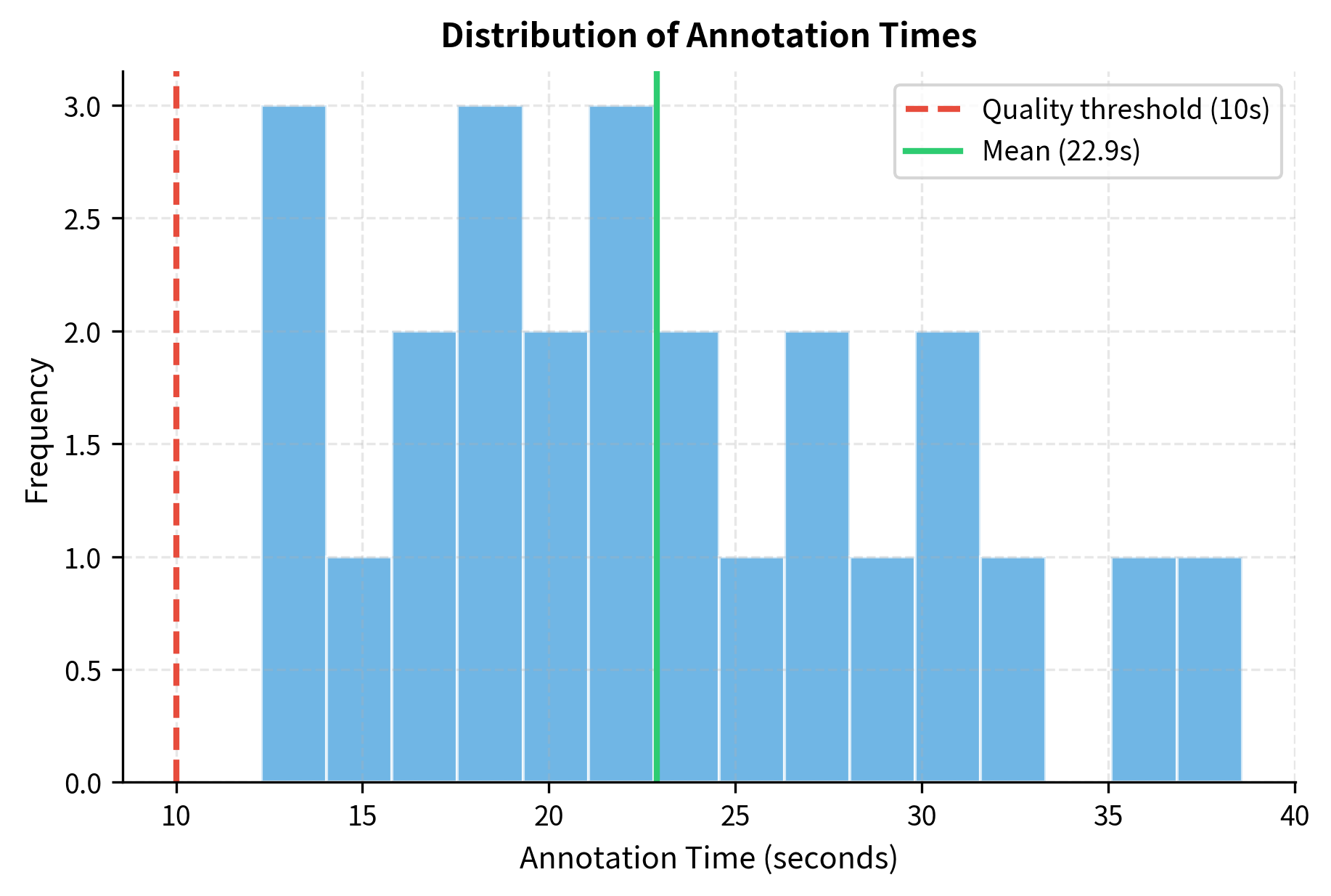
Annotation Time Tracking
Recording how long annotators spend on each comparison provides useful quality signals. Suspiciously fast annotations (under 10 seconds for long responses) may indicate satisficing or random selection. Very slow annotations may indicate difficult comparisons where the annotator is uncertain.
Time data helps identify both unreliable annotators and ambiguous comparison pairs that might need clearer guidelines or should be excluded from training.
Comparison Design
The prompts and responses used in preference collection determine what behaviors the resulting model will learn. Poor comparison design limits what alignment can achieve. This section explores how to construct comparisons that provide maximal information about the quality distinctions we care about.
Prompt Selection
The prompts used for preference collection should cover the distribution of tasks the model will encounter in deployment. This requires careful consideration of:
- Domain coverage: Instructions should span different use cases: creative writing, coding assistance, factual questions, advice requests, analysis tasks. A dataset heavily weighted toward one domain will produce a model with uneven capabilities.
- Difficulty distribution: Including both simple and complex prompts ensures the model learns preferences across difficulty levels. Easy prompts (like basic factual questions) may have clear "correct" answers, while harder prompts (like nuanced ethical dilemmas) require more sophisticated judgment.
- Edge cases: Deliberately including prompts that probe potential failure modes: ambiguous requests, requests with hidden assumptions, requests that might elicit harmful content. These adversarial prompts help the model learn appropriate boundaries.
Response Generation
The responses being compared typically come from the model being aligned, or an earlier version of it. The generation strategy affects what the model can learn:
- Temperature diversity: Generating responses at different temperatures produces variety. High-temperature samples may include creative but risky outputs; low-temperature samples may be safer but more generic. Comparing across temperatures helps the model learn when creativity versus caution is appropriate.
- Multiple model versions: Comparing outputs from the current model against a previous version, or against a different model entirely, creates informative contrasts. If annotators consistently prefer GPT-4's responses over the model being trained, those comparisons teach the model to emulate GPT-4's style.
- Intentional degradation: Some datasets deliberately include low-quality responses (truncated, factually wrong, or stylistically poor) to establish clear negative examples. These "easy" comparisons ensure the model learns basic quality signals, though they provide less information than comparisons between two reasonable responses.
Contrastive Pair Generation
The most informative comparisons involve responses that differ in specific ways. Rather than comparing a clearly good response to a clearly bad one, effective datasets include pairs where:
- Both responses are reasonable but differ in style or emphasis
- One response is more complete, the other more concise
- One response directly answers the question, the other provides useful context first
- Both responses are correct but one is more clearly explained
These contrastive pairs force annotators (and later, the reward model) to make fine-grained distinctions about quality. The key insight is that we learn most from close comparisons where the distinction is subtle, not from obvious cases where any reasonable annotator would agree.
Annotator Guidelines
Clear guidelines are essential for consistent preference judgments. Without explicit criteria, different annotators will apply different standards, introducing noise into the dataset. Guidelines serve as a shared reference point that helps annotators calibrate their judgments to a common standard.
Defining Quality Criteria
Guidelines should specify what annotators should consider when comparing responses. These criteria operationalize our abstract notion of "quality" into concrete factors that annotators can evaluate. Common criteria include:
- Helpfulness: Does the response actually help you accomplish your goal? Does it answer the question asked, or does it dodge the question? Does it provide actionable information?
- Accuracy: Is the information correct? For factual claims, is there evidence? For reasoning, are the logical steps valid?
- Clarity: Is the response easy to understand? Is it well-organized? Does it explain technical concepts appropriately for the apparent audience?
- Harmlessness: Does the response avoid providing dangerous information? Does it refuse inappropriate requests appropriately without being unnecessarily restrictive?
- Honesty: Does the response acknowledge uncertainty when appropriate? Does it avoid claiming capabilities the model doesn't have?
Guidelines should specify how to weigh these criteria when they conflict. For example: "If one response is more helpful but slightly less accurate, prefer the accurate response. Accuracy takes priority over helpfulness."
Handling Ambiguous Cases
Some comparisons have no clear winner. Guidelines should address:
- Ties: When should annotators select "tie" or "no preference"? Some projects discourage ties to maximize signal; others allow ties to avoid forcing arbitrary choices. The guideline should be explicit.
- Different but equal: Two responses might take different valid approaches. "If both responses would satisfy you and neither has clear advantages, you may select 'tie' or choose based on personal preference, but note your reasoning."
- Partial quality: One response might be better on some criteria and worse on others. Guidelines should specify how to resolve such tradeoffs.
Calibration Examples
Including worked examples in the guidelines helps annotators calibrate their judgments. Each example should show:
- The prompt
- Two responses
- The correct choice
- Explanation of why that choice is correct
Effective calibration examples include:
- Clear cases that establish baseline expectations
- Close calls that illustrate subtle distinctions
- Traps where surface features (length, formality) might mislead annotators away from the genuinely better response
Documenting Edge Cases
As annotation proceeds, edge cases emerge that guidelines didn't anticipate. Maintaining a living FAQ or edge case document helps ensure consistent handling:
Q: What if one response is correct but uses informal language while
   the other is wrong but sounds professional?
A: Prefer correctness over tone. Factual accuracy always takes
   priority over stylistic preferences.

Q: What if the prompt asks for something unethical?
A: Prefer the response that appropriately declines while still
   being respectful to you.
Quality Control and Agreement
Preference data quality directly impacts alignment quality. Multiple mechanisms help ensure the data is reliable. This section explores how to measure agreement between annotators and what those measurements tell us about our data.
Inter-Annotator Agreement
Having multiple annotators label the same comparison allows measurement of agreement. Common metrics include:
Raw agreement rate: the percentage of comparisons where annotators chose the same response. For binary choices, random agreement is 50%, so rates should substantially exceed this.
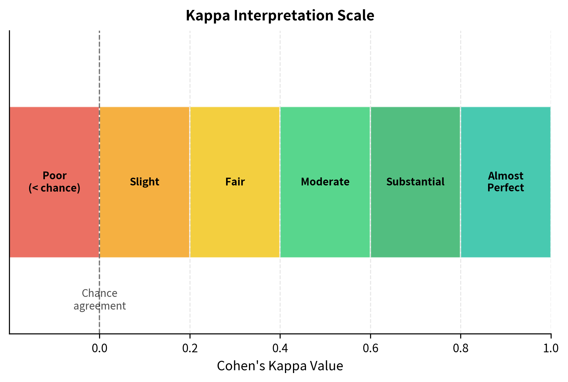
Cohen's Kappa: Raw agreement rate has a significant limitation: it does not account for the possibility that annotators might agree purely by chance. If two annotators are each selecting randomly, they would still agree about half the time on binary choices. We need a metric that tells us how much better than chance our annotators are agreeing.
Cohen's Kappa addresses this need by measuring inter-annotator agreement while accounting for the probability of chance agreement. The core insight is that we want to measure the agreement that goes beyond what we would expect from random labeling. The formula is:
where:
- : the Cohen's Kappa coefficient
- : the observed agreement (the proportion of items where annotators actually agreed)
- : the expected agreement by chance (derived from the marginal distributions of annotator choices)
- : the agreement achieved beyond chance
- : the maximum possible agreement beyond chance
To understand this formula intuitively, consider what each component represents. The numerator, , captures how much agreement we observed beyond what chance would predict. If our annotators agreed on 80% of items () but random labeling would have yielded 50% agreement (), then the numerator is . This represents the "extra" agreement that comes from annotators actually agreeing on quality judgments rather than randomly clicking buttons.
The denominator, , represents the maximum possible improvement over chance. If chance agreement is 50%, then the best we could do beyond chance is the remaining 50% (achieving 100% agreement). This normalization ensures that kappa values are comparable across situations with different chance agreement levels.
The formula thus computes what fraction of the possible improvement over chance our annotators actually achieved. A value of 0 implies agreement no better than chance, while 1 implies perfect agreement. Values above 0.6 generally indicate substantial agreement, while values above 0.8 indicate near-perfect agreement. Negative values are possible and indicate agreement worse than chance, which might occur if annotators are systematically misunderstanding the task.
Krippendorff's Alpha: A more flexible agreement measure that handles multiple annotators and missing data.
Typical preference datasets achieve 70-80% pairwise agreement, meaning annotators agree on 7-8 out of 10 comparisons. Perfect agreement is neither expected nor desirable, as it would suggest the comparisons are too easy to provide useful training signal.
Disagreement Analysis
When annotators disagree, understanding why is informative:
- Ambiguous prompts: The prompt may be interpreted differently by different annotators
- Subjective criteria: Some preferences are genuinely personal (formal vs. casual tone)
- Criteria conflicts: One annotator weighted helpfulness higher; another weighted accuracy
- Annotation errors: One annotator misread a response or made a mistake
Systematically categorizing disagreements can reveal problems with guidelines or prompts that can be corrected.
Quality Assurance Mechanisms
Several mechanisms help maintain data quality throughout collection:
- Gold questions: Include comparisons with known correct answers (e.g., one response is clearly harmful, one is clearly appropriate). Annotators who miss gold questions can be flagged for retraining or removal.
- Consistency checks: Show the same comparison twice (with response order flipped) and check whether the annotator's choice is consistent.
- Feedback loops: Regular meetings with annotators to discuss difficult cases, clarify guidelines, and address systematic problems.
- Statistical outlier detection: Identify annotators whose judgments systematically differ from the majority. Some divergence is expected, but extreme outliers may indicate confusion or low effort.
Implementing Preference Data Collection
Let's implement a simple preference data processing pipeline that demonstrates key concepts.
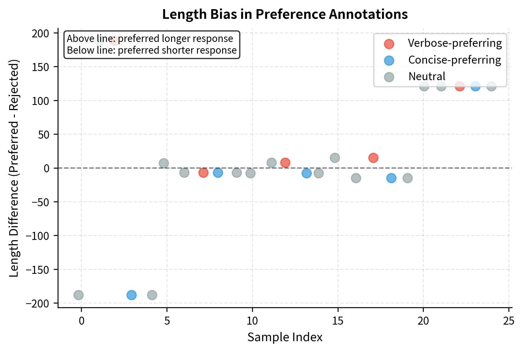
Now let's create some example preference data that illustrates common patterns:
The dataset contains 25 samples distributed across 5 prompts and 5 annotators. This scale is sufficient to demonstrate the data structures and analysis pipelines, though real-world datasets typically contain thousands of examples.
Let's analyze the preference distribution and look for potential biases:
The distribution reveals a mix of preferences, with some annotators showing distinct biases. The length correlation metrics help identify whether annotators systematically favor longer responses, a common quality issue where verbosity is mistaken for helpfulness.
Now let's compute inter-annotator agreement using Cohen's Kappa:
The agreement analysis reveals important patterns. Annotators with different biases (verbose vs. concise preferences) show lower agreement with each other, while annotators with similar tendencies agree more often. This illustrates why understanding annotator characteristics matters for data quality.
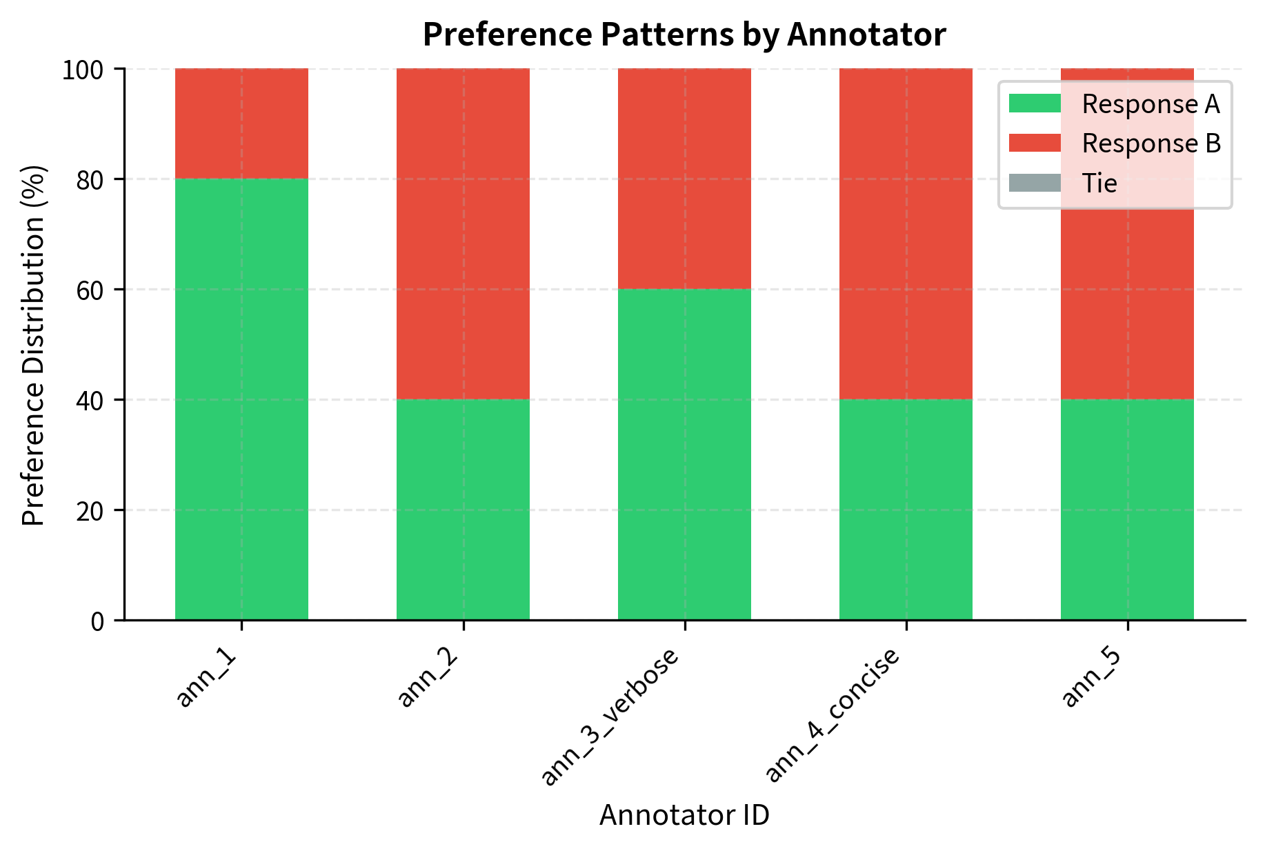
Let's visualize the preference patterns across annotators:
Converting to Training Format
Preference data must be converted to a format suitable for training reward models. The standard format pairs each prompt with its chosen and rejected responses:
This format directly supports the reward modeling objective we'll cover in upcoming chapters: the reward model learns to assign higher scores to chosen responses than rejected ones.
Key Parameters
The key parameters for the preference data structures are:
- prompt: The instruction or question provided to the model.
- response_a/response_b: The two model outputs presented for comparison.
- preference: The annotator's judgment ("a", "b", or "tie").
- annotator_id: Unique identifier for the annotator, used to track individual biases and agreement.
Real-World Preference Datasets
Several public preference datasets demonstrate these principles at scale:
Anthropic HH-RLHF: Contains conversations rated for helpfulness and harmlessness. Annotators compared assistant responses in multi-turn dialogues, focusing on whether responses were genuinely helpful without being harmful.
OpenAssistant: A crowdsourced dataset with multi-level rankings. Annotators ranked multiple responses per prompt, and the data includes quality flags and annotator metadata.
Stanford Human Preferences (SHP): Derived from Reddit, where upvotes serve as implicit preference signals. This represents a different collection paradigm using naturally occurring human feedback rather than explicit annotation.
UltraFeedback: Uses GPT-4 to provide preference judgments, representing the AI feedback approach where a stronger model labels data for training weaker models.
Each dataset makes different design choices that affect what behaviors the resulting models learn. Understanding these choices helps practitioners select appropriate data for their alignment goals.
Limitations and Impact
Human preference data, while powerful, has fundamental limitations that shape what alignment can achieve.
The most significant challenge is that preferences are not ground truth. Different annotators have different values, backgrounds, and interpretations. A response one annotator finds helpful might strike another as condescending. A response deemed harmless by one might seem problematic to another based on cultural context. When we aggregate preferences, we're constructing a statistical summary of diverse opinions, not discovering objective facts about quality. This means aligned models reflect a particular distribution of human views, not some universal standard.
Annotator demographics matter enormously. Most preference datasets are labeled by workers in specific geographic regions, typically English-speaking and with access to the labeling platforms. These annotators may not represent the global user base of language models. Preferences about appropriate humor, cultural references, or sensitive topics vary across populations. Models aligned to one population's preferences may behave inappropriately for others.
The comparison format itself limits what preferences can be expressed. Pairwise comparisons work well for choosing between similar responses but struggle to capture the full structure of preferences. An annotator might think both responses are terrible, or both are excellent, but the interface forces a choice between them. Some preference relationships are intransitive (A preferred to B, B preferred to C, but C preferred to A), which the standard frameworks cannot represent.
Scale remains a persistent challenge. Collecting high-quality preference data is expensive and slow. Annotators must read lengthy responses carefully, consider multiple quality dimensions, and make difficult judgments. Rushing this process degrades quality, but thorough annotation limits dataset size. This tension between quality and quantity affects all preference datasets.
Despite these limitations, human preference data has enabled remarkable progress in alignment. The RLHF pipeline, built on preference data, transformed language models from capable but unreliable systems into assistants that follow instructions, acknowledge uncertainty, and refuse harmful requests. The preference data approach succeeded where explicit rules failed, precisely because preferences encode implicit knowledge that resists formalization.
Summary
Human preference data provides the empirical foundation for language model alignment. Rather than specifying desired behavior through rules, we collect examples of humans choosing between model outputs, then use these choices to guide model behavior.
The key elements of preference data collection include:
- Collection format: Pairwise comparisons dominate due to cognitive simplicity and theoretical grounding, though rankings and ratings offer alternatives
- Interface design: Randomized response positions, consistent formatting, and hidden model identity prevent systematic biases
- Comparison design: Prompts should cover expected use cases, and response pairs should include informative contrasts, not just easy choices
- Annotator guidelines: Clear criteria for quality dimensions (helpfulness, accuracy, harmlessness) with worked examples help ensure consistent judgments
- Quality control: Inter-annotator agreement metrics, gold questions, and outlier detection maintain data reliability
The decisions made during preference collection affect the entire alignment pipeline. In the next chapter, we'll see how the Bradley-Terry model provides a principled framework for converting pairwise preference data into reward scores.
Quiz
Ready to test your understanding? Take this quick quiz to reinforce what you've learned about human preference data collection for language model alignment.

Comments