

Learn how the Bradley-Terry model converts pairwise preferences into consistent rankings. Foundation for reward modeling in RLHF and Elo rating systems.

This article is part of the free-to-read Language AI Handbook
Choose your expertise level to adjust how many terms are explained. Beginners see more tooltips, experts see fewer to maintain reading flow. Hover over underlined terms for instant definitions.
Bradley-Terry Model
In the previous chapter, we explored how human preference data is collected through pairwise comparisons: annotators see two model responses and indicate which one they prefer. But raw preference counts aren't directly useful for training. If response A was preferred over response B in 73% of comparisons, and response B was preferred over response C in 68% of comparisons, how much better is A than C? How do we convert these pairwise judgments into consistent quality scores that can guide model optimization?
The Bradley-Terry model, developed by Ralph Bradley and Milton Terry in 1952, provides an elegant statistical framework for exactly this problem. Originally designed for ranking chess players and sports teams, it assumes each item has a latent "strength" parameter, and the probability of one item beating another depends only on the ratio of their strengths. This simple assumption leads to a powerful model that converts noisy pairwise comparisons into consistent, transitive rankings.
For LLM alignment, the Bradley-Terry model is foundational. As we'll see in the upcoming chapter on Reward Modeling, the reward model training objective is directly derived from the Bradley-Terry likelihood. Understanding this model deeply will clarify why reward models are trained the way they are, and why later techniques like Direct Preference Optimization (DPO) can eliminate the need for explicit reward modeling altogether.
The Pairwise Comparison Framework
Consider a setting where we have items (in our case, model responses) that we want to rank based on human preferences. We don't observe quality scores directly; instead, we observe the outcomes of pairwise comparisons. When comparing items and , a human annotator chooses one as better. This setup reflects how humans naturally make judgments: rather than assigning absolute quality scores on some numerical scale, people find it far easier to simply say which of two options they prefer. The challenge lies in synthesizing these individual binary decisions into a coherent global ranking.
A pairwise comparison is a judgment where an evaluator observes two items and selects which one is superior according to some criterion. The comparison produces a binary outcome: either item wins or item wins.
The key insight of the Bradley-Terry model is that we can explain these observed preferences through latent strength parameters. Each item has an associated strength that represents its underlying quality. We never observe these strengths directly. Instead, we must infer them from the pattern of wins and losses across many comparisons. Items with higher strength values are better, and when two items are compared, the one with higher strength is more likely to win, but not guaranteed to win, which accounts for noise in human judgments. This probabilistic view is essential: it acknowledges that human preferences contain randomness, whether from inconsistency, variation in attention, or genuine differences of opinion among annotators.
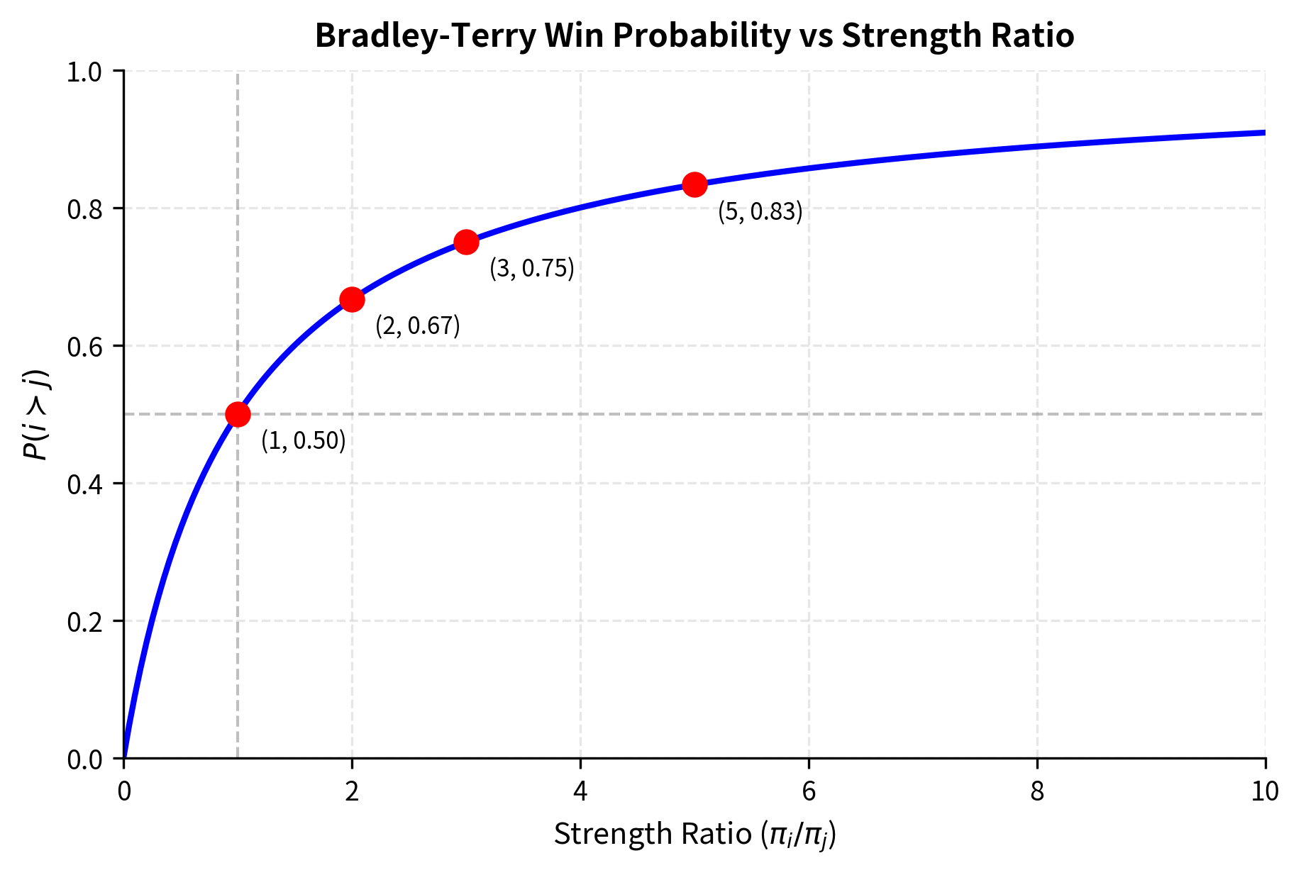
The fundamental assumption is that the probability of item being preferred over item depends only on the ratio of their strengths:
where:
- : the probability that item is preferred over item
- : the latent strength parameters of items and (must be positive)
This formula has an intuitive interpretation that makes it easy to reason about. Consider first the case where : substituting into the formula gives . This confirms our intuition that equally strong items have equal probability of being chosen. Now consider a more extreme case: if , then . An item three times as strong wins 75% of the time. Notice that the absolute magnitudes of the strengths do not matter, only their ratio. Whether we have strengths of 3 and 1, or 300 and 100, the predicted win probability remains the same. This ratio-based formulation captures the intuitive notion that what matters is relative quality, not absolute quality.
The Log-Linear Form
While the ratio formulation is intuitive, a more convenient parameterization uses log-strengths. This transformation opens up powerful connections to logistic regression and makes optimization considerably easier. Let . Since strengths must be positive, the log-strength can be any real number, which is mathematically more convenient for optimization algorithms. We can now derive the equivalent expression in terms of these log-strengths:
where:
- : the log-strength parameters of items and
- : the latent strength parameters ()
- : the sigmoid function
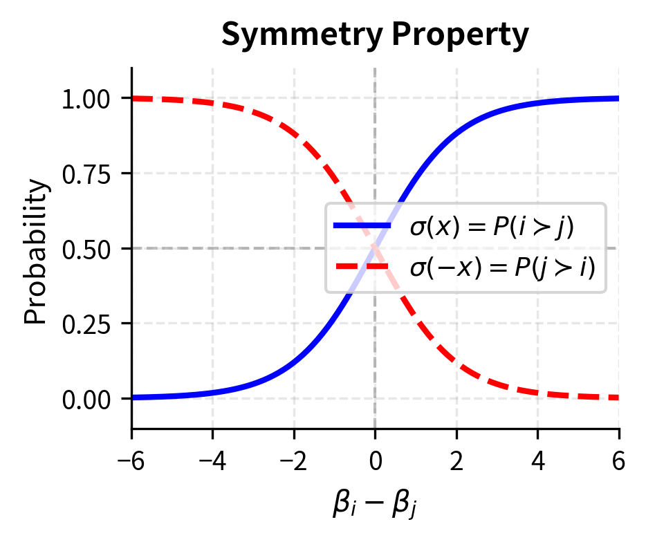
The function is the standard sigmoid familiar from logistic regression and neural network activations (as covered in Part VII on Activation Functions). The sigmoid function has several properties that make it ideal for representing probabilities. It maps any real number to the interval , ensuring valid probabilities. It is symmetric around zero, meaning , which captures the natural symmetry of pairwise comparisons: the probability that beats equals one minus the probability that beats . The sigmoid is also smooth and differentiable everywhere, which enables gradient-based optimization.
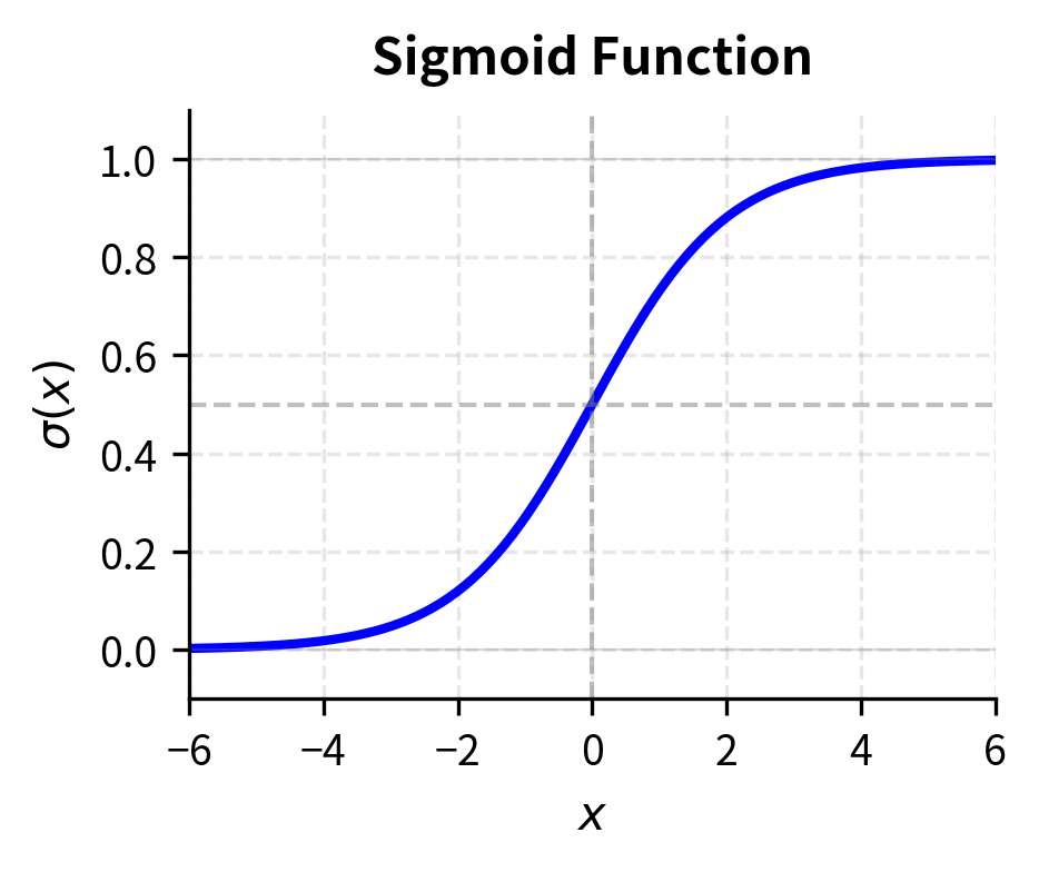
This log-linear form reveals that the Bradley-Terry model is equivalent to logistic regression where the probability of beating depends on the difference in their log-strengths. The sigmoid function ensures probabilities stay between 0 and 1, with the midpoint at 0.5 when . This equivalence to logistic regression is more than a mathematical curiosity: it means we can leverage decades of research on logistic regression, including efficient optimization algorithms, regularization techniques, and statistical theory about confidence intervals and hypothesis tests.
The probability that item is preferred over item in the Bradley-Terry model is:
where:
- : the log-strength parameters of the two items
- : the sigmoid function mapping the difference to a probability
Preference Strength and Transitivity
A crucial property of the Bradley-Terry model is that it produces transitive preferences. Transitivity means that if A is better than B, and B is better than C, then A must be better than C. If we know how often A beats B, and how often B beats C, the model automatically determines how often A beats C. This follows directly from the parameterization, and understanding why reveals something deep about the model's structure.
The transitivity arises because each item has a single strength parameter that governs all of its comparisons. When we estimate , , and , these values must simultaneously explain the A-versus-B comparisons, the B-versus-C comparisons, and the A-versus-C comparisons. The model cannot assign different "strengths" to A depending on which item it is facing. This constraint forces global consistency.
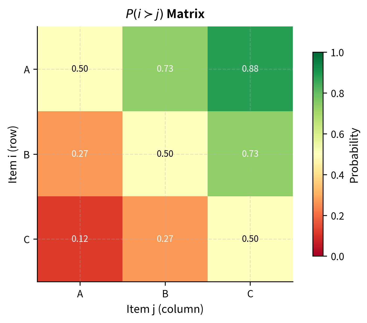
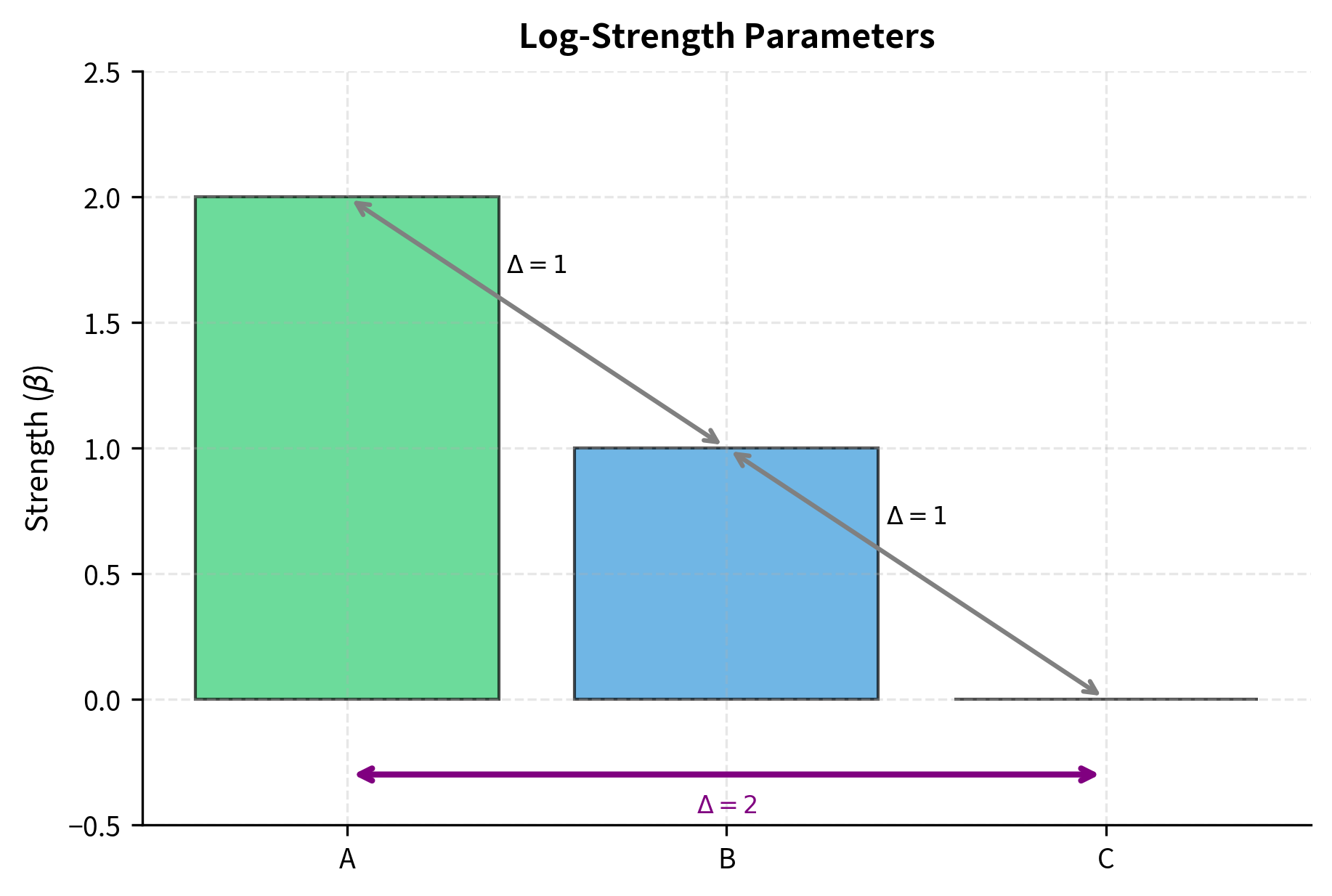
Consider three items with strengths , , and . The pairwise probabilities are:
where:
- : the example strengths ()
- : the probability A beats B
- : the sigmoid function applied to strength differences
Notice that even though A and B have the same preference probability over their respective "next" item (both beat their weaker neighbor about 73% of the time), A has a much higher probability of beating C than B does of beating C. The strengths compose properly: the gap between A and C is the sum of the gaps between A and B and between B and C. Specifically, . This additive property of log-strengths is what makes the model so elegant. Strength differences accumulate predictably across chains of comparisons.
This transitivity is a feature, not a bug. It forces the model to find a consistent ranking that best explains all observed comparisons, even when individual comparisons contain noise or contradictions. If humans sometimes prefer B over A, the model can still conclude A is better overall if A wins more often than it loses. The model essentially averages over the noise to find the underlying signal. However, as we will discuss later, this built-in transitivity can also be a limitation when human preferences genuinely violate transitivity.
The Bradley-Terry Likelihood
To estimate the strength parameters from observed comparisons, we use maximum likelihood estimation. The goal is to find the parameter values that make the observed data most probable. This is a principled statistical approach: among all possible strength assignments, we seek the one that best explains what we actually saw happen in the comparisons.
Suppose we have a dataset of pairwise comparisons, where comparison involves items and , and item was chosen as the winner. The key assumption is that each comparison is independent, which is reasonable if different annotators make different comparisons, or if the same annotator's judgments don't depend on what they saw before.
The likelihood of observing this data under the Bradley-Terry model is:
where:
- : the likelihood of the observed dataset given parameters
- : the total number of pairwise comparisons
- : indices of the winning and losing items in the -th comparison
- : the sigmoid function mapping the strength difference to a probability
The product form arises from independence: the probability of seeing all the comparisons we saw is the product of the probabilities of each individual comparison. Each term in the product is the Bradley-Terry probability that the actual winner wins, given the current strength parameters. The goal of maximum likelihood estimation is to find the values that make this product as large as possible.
Taking the log-likelihood converts the product into a sum, which is more convenient both analytically and computationally:
where:
- : the log-likelihood function to be maximized
- : the total number of comparisons
- : indices of the winning and losing items in comparison
- : log-strength parameters for the winner and loser
- : the log-sigmoid equivalent to the negative softplus function
This is the negative of the binary cross-entropy loss where we're predicting that the winner should win. The connection to binary cross-entropy is important: it means that training a Bradley-Terry model is computationally identical to training a logistic regression classifier. The maximum likelihood estimates are found by maximizing this expression with respect to , typically using gradient-based optimization methods like gradient descent or L-BFGS.
The Identifiability Issue
There's a subtlety that arises when we try to estimate Bradley-Terry parameters: the model has a scale and location invariance. If we add a constant to all parameters, the probabilities don't change:
where:
- : an arbitrary constant added to all log-strength parameters
- : the log-strength parameters
- : the sigmoid function
This invariance occurs because the sigmoid only depends on differences between parameters, not on their absolute values. The constant cancels out in the subtraction. Mathematically, this means the parameters are not uniquely identifiable; there are infinitely many solutions that produce the same likelihood. If is a solution, then so is , and so is . All these solutions make identical predictions.
To resolve this ambiguity, we typically fix one parameter (e.g., ) or add a constraint like . This anchoring doesn't affect the relative rankings or prediction probabilities. It simply pins down the arbitrary location of the parameter scale so that optimization algorithms converge to a unique solution. The choice of anchor is arbitrary: we could anchor any item at any value, and the relative differences would remain the same.
Connection to Elo Ratings
If the Bradley-Terry model sounds familiar, it should. The Elo rating system, used to rank chess players and now common in competitive gaming, is a Bradley-Terry model in disguise. Understanding this connection illuminates both systems and explains why Elo ratings have become standard for comparing language models.
Elo ratings are typically scaled so that a 400-point difference corresponds to a 10:1 expected score ratio. This scaling was chosen for historical and practical reasons: it produces ratings that are easy to interpret and compare. A rating difference of 400 points means the stronger player is expected to score about 10 points for every 1 point the weaker player scores over many games.
In standard Elo, the expected score of player against player is:
where:
- : the expected score (win probability) of player
- : the Elo ratings of players and
- : the scaling factor where a difference of 400 points implies a 10:1 odds ratio
The use of base-10 exponentials rather than natural exponentials is purely conventional: Arpad Elo chose this scaling when he developed the system in the 1960s because it produced convenient numbers for chess ratings.
We can rewrite this in terms of the sigmoid function by converting the base-10 exponential to base-:
where:
- : the expected score (win probability) for player
- : the natural logarithm of 10
- : the standard sigmoid function
This derivation demonstrates that the Elo rating is just a scaled version of the Bradley-Terry log-strength parameter. Specifically, if is the Bradley-Terry parameter, then the corresponding Elo rating is . The mathematical structure is identical; only the units differ.
The connection matters because Elo-style ratings are now used to evaluate LLMs. Platforms like LMSYS Chatbot Arena use Elo ratings computed from human preference comparisons to rank models. When you vote for which model response you prefer, these votes become pairwise comparisons that update the models' Elo ratings. The Bradley-Terry framework provides the statistical foundation for these rankings, ensuring that the ratings are consistent and interpretable.
Worked Example
Let's work through a concrete example to solidify these concepts and see how the mathematics plays out with real numbers. Suppose we have three model responses (A, B, C) and the following comparison outcomes:
| Comparison | Winner | Occurrences |
|---|---|---|
| A vs B | A | 7 |
| A vs B | B | 3 |
| B vs C | B | 8 |
| B vs C | C | 2 |
| A vs C | A | 9 |
| A vs C | C | 1 |
We'll set as our anchor. This choice is arbitrary, but it resolves the identifiability issue and allows us to interpret the other parameters as "how much better than C" each item is. The log-likelihood function aggregates all our comparison data:
where:
- : the log-likelihood function aggregating all comparisons
- : the observed counts (e.g., A beats B 7 times)
- : the sigmoid function mapping strength differences to probabilities
- : the unknown log-strength parameters
- : the fixed anchor value for item C ()
Each term in this sum corresponds to a set of comparisons. The first term, , contributes to the likelihood every time A beats B, which happened 7 times. The second term accounts for the 3 times B beat A. Notice how the symmetry of preferences emerges: when A beats B, we use , and when B beats A, we use .
To find the maximum, we take derivatives and set them to zero. We rely on the derivative property of the log-sigmoid function: . This elegant result comes from the chain rule and the fact that .
Applying the chain rule to the terms involving :
- When A wins (e.g., against B): The term is . The derivative is .
- When A loses (e.g., against B): The term is . The derivative is , which simplifies to .
Substituting the counts into the gradient equation for :
where:
- : the gradient of the log-likelihood with respect to
- : the log-strength parameters
- : the sigmoid function
- : the derivative of the term for wins
- : the derivative of the term for losses
Using the property that and :
where:
- : the probability that B beats A
- : the probability that C beats A (equivalent to )
- : the log-strength parameters
- : the sigmoid function
The gradient equations don't have a closed-form solution, so we use iterative optimization. Unlike linear regression, where we can solve for parameters directly, the nonlinearity of the sigmoid means we must use numerical methods. Let's implement this in code.
Code Implementation
We'll implement Bradley-Terry estimation from scratch using gradient descent, then show how it's applied in practice.
Now let's define the negative log-likelihood function that we want to minimize:
We also need the gradient for efficient optimization:
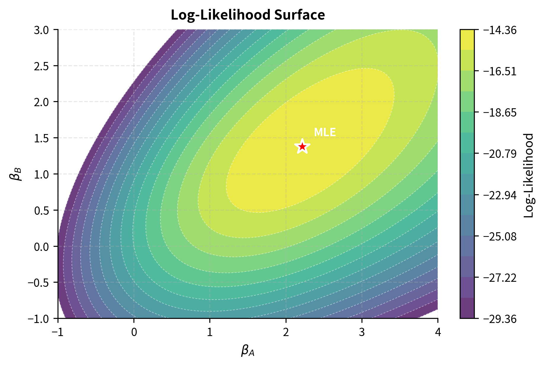
Now let's optimize to find the maximum likelihood estimates:
The estimated coefficients indicate that Item A is the strongest, followed by Item B, with Item C as the baseline. The optimization successfully converged to these maximum likelihood estimates.
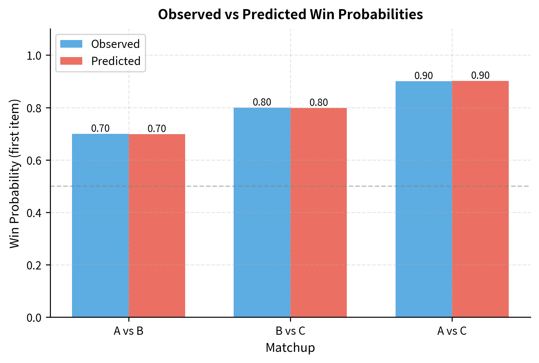
Let's verify these estimates by computing the predicted win probabilities:
The model closely matches the observed frequencies. Now let's convert these to Elo-style ratings for interpretability:
The ratings align with our expectations: Item A has the highest rating, reflecting its dominance in the pairwise comparisons. A difference of approximately 200 points between A and B suggests a strong win probability for A.
Visualizing the Preference Surface
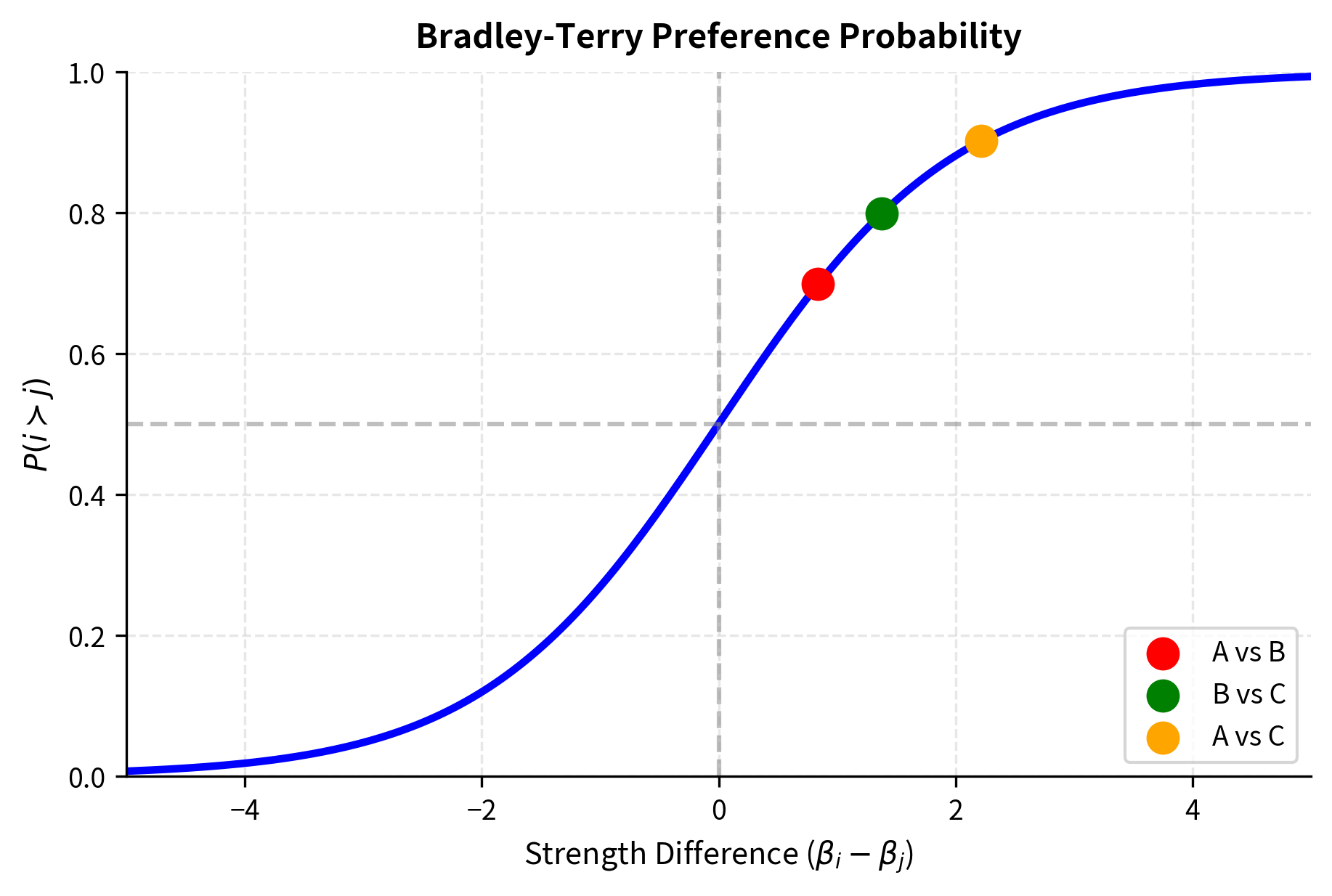
Let's visualize how the Bradley-Terry probability varies with the strength difference:
The curve shows the characteristic sigmoid shape. When strengths are equal (), the win probability is exactly 0.5. Small strength differences near zero produce probability changes close to linear, while large differences saturate toward 0 or 1.
Handling Real Preference Data
In practice, preference data comes as individual comparison records rather than aggregated counts. Let's implement a more realistic version that handles raw comparison logs:
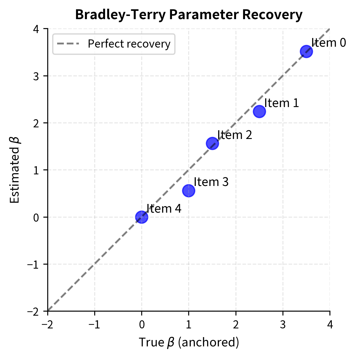
Let's test this implementation with simulated preference data:
The estimated parameters closely recover the true values, demonstrating that the Bradley-Terry model can reliably learn latent strengths from noisy pairwise comparisons.
Visualizing Parameter Recovery
Connection to Reward Modeling
The Bradley-Terry model is the foundation of reward model training in RLHF. Understanding this connection reveals why reward models are trained the way they are and illuminates the mathematical underpinnings of alignment techniques. Recall from the previous chapter that preference data consists of pairs where is the preferred response and is the dispreferred response to the same prompt .
A reward model assigns a scalar score to each prompt-response pair. This score represents the model's estimate of how good the response is for that particular prompt. The key insight is that we can interpret this reward as a Bradley-Terry strength parameter: the probability that response is preferred over should follow the Bradley-Terry formula:
where:
- : the preferred (winning) and dispreferred (losing) responses
- : the prompt or context
- : the reward model parameterized by weights
- : the sigmoid function converting the reward difference into a probability
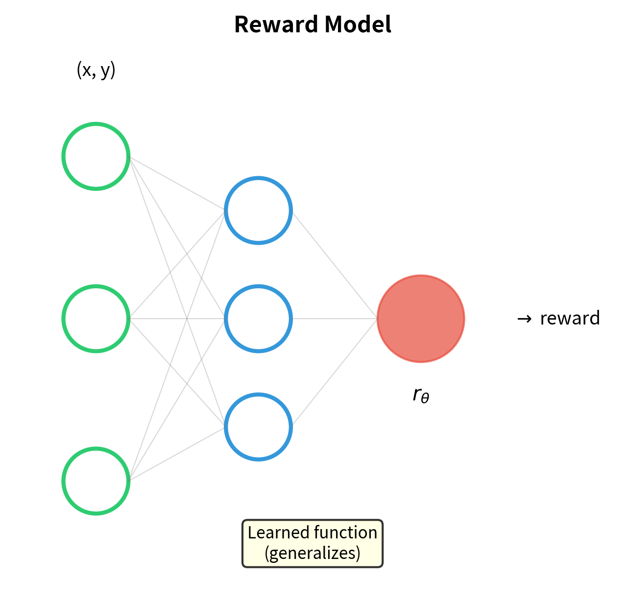
This formulation says that the probability of preferring one response over another depends on the difference in their reward scores, passed through a sigmoid. Responses with higher rewards are more likely to be preferred, but the relationship is probabilistic, allowing for noise in human judgments. Training the reward model to maximize this probability is equivalent to Bradley-Terry maximum likelihood estimation, except now the strength parameters are neural network outputs rather than fixed scalars. Instead of learning one number per item, we learn a function that can assign rewards to any prompt-response pair.
The loss function for reward model training is:
where:
- : the loss function to minimize (negative log-likelihood)
- : the dataset of preference pairs
- : the expectation over samples drawn from the dataset
- : the sigmoid function
- : the reward model output for input and response
- : the preferred and dispreferred responses
This is exactly the Bradley-Terry negative log-likelihood, with the expectation taken over the preference dataset. The connection is direct: minimizing this loss trains the neural network to produce reward scores that best explain the observed human preferences according to the Bradley-Terry model. We'll explore the full details of reward model architecture and training in the next chapter, but understanding Bradley-Terry makes the training objective transparent: we're fitting a neural network to predict comparison outcomes.
Limitations and Impact
The Bradley-Terry model makes strong assumptions that don't always hold in practice. The most significant is the independence from irrelevant alternatives: the probability that A beats B doesn't depend on what other items exist in the comparison set. This means if you're comparing responses A and B, introducing a third response C shouldn't change how humans compare A to B. In reality, context effects like anchoring and decoy effects violate this assumption.
The model also assumes preferences are governed by a single latent dimension: each item has one "strength" value that determines all its comparisons. Human preferences for text are often multidimensional: a response might be more helpful but less safe, or more creative but less accurate. A single scalar reward compresses these tradeoffs into one number, potentially losing important information. Research into multi-objective RLHF attempts to address this limitation by learning separate reward models for different attributes.
Another challenge is intransitivity in human preferences. The Bradley-Terry model enforces transitivity by construction: if A is stronger than B and B is stronger than C, then A must be stronger than C. But humans sometimes exhibit cycles: preferring A over B, B over C, yet C over A. These cycles can arise from different annotators having different preferences, or from the same annotator weighing different factors in different comparisons. The Bradley-Terry model smooths over these inconsistencies, which is usually desirable but can mask systematic disagreements.
Despite these limitations, the Bradley-Terry model has had enormous impact on LLM alignment. Its simplicity makes it computationally tractable to train reward models on millions of preference comparisons. The resulting reward scores provide the training signal for PPO and other policy optimization algorithms. More recently, the mathematical connection between reward models and the Bradley-Terry likelihood enabled Direct Preference Optimization, which we'll cover later in this part. DPO derives an implicit reward model from the policy itself, eliminating the need for separate reward model training while still optimizing the same Bradley-Terry objective.
Summary
The Bradley-Terry model provides a principled framework for converting pairwise comparison data into consistent quality scores. Its core assumptions are:
- Each item has a latent strength parameter
- The probability that item beats item is
- Parameters are learned by maximum likelihood estimation
Key insights from this chapter:
- Log-linear form: The Bradley-Terry probability is a sigmoid of the strength difference, making it equivalent to logistic regression on pairwise comparisons
- Transitivity by design: The model automatically produces transitive rankings, which is both a feature (consistency) and a limitation (can't represent true intransitivity)
- Identifiability: Only differences in strength matter, so we need to anchor one parameter
- Connection to Elo: The Elo rating system is a scaled Bradley-Terry model
- Foundation for reward modeling: The reward model training objective is exactly the Bradley-Terry likelihood with neural network-parameterized strengths
In the next chapter on Reward Modeling, we'll see how this framework scales to neural networks that can generalize across prompts and responses, providing the dense training signal needed for RLHF.
Quiz
Ready to test your understanding? Take this quick quiz to reinforce what you've learned about the Bradley-Terry model and its role in preference learning.

Comments