Reward Modeling: Building Preference Predictors for RLHF

In the previous chapter, we explored the Bradley-Terry model and how it provides a probabilistic framework for converting pairwise human preferences into a consistent scoring system. Now we turn to the practical question: how do we build a neural network that learns to predict these preferences?

A reward model is a neural network that takes a prompt and response as input and outputs a scalar score indicating how "good" that response is according to human preferences. This model serves as a proxy for human judgment, allowing us to provide dense feedback signals during reinforcement learning without requiring a human to evaluate every generated response. The reward model sits at the heart of RLHF: it translates sparse, noisy human preferences into a continuous signal that can guide policy optimization.

Building an effective reward model requires careful consideration of architecture choices, loss functions, and evaluation methods. The model must generalize from a limited set of human comparisons to accurately score responses it has never seen before, including responses generated by future versions of the language model being trained. This chapter covers the complete pipeline from architecture design through training and evaluation.

The standard approach to building a reward model starts with a pretrained language model and adds a simple regression head that maps the final hidden states to a scalar reward. This design philosophy reflects a key insight: rather than learning to understand language from scratch, we can leverage the rich representations already encoded in models that have been trained on vast text corpora. The pretrained model provides the linguistic foundation, while the new regression head learns to interpret those representations through the lens of human preferences.

Reward models typically use the same architecture family as the policy model they will train. If you're using RLHF to fine-tune a 7B parameter LLaMA model, your reward model might be initialized from the same pretrained checkpoint or a similar model in the family. This architectural alignment ensures the reward model can process the same input representations and has similar language understanding capabilities. The choice is not arbitrary: when the reward model shares the same "vocabulary" of internal representations as the policy model, it can more accurately evaluate the subtle qualities of responses that the policy might generate.

The key modification is replacing or augmenting the language modeling head. Instead of predicting the next token, we need to output a single scalar value that represents the quality of the entire response. This transformation converts a generative model into an evaluative one, shifting from the question "what comes next?" to "how good is this?"

The core architectural question for reward modeling is this: how do we collapse an entire sequence of hidden states, one for each token in the prompt and response, into a single number that captures the overall quality? The solution involves selecting a representative hidden state and projecting it down to a scalar through a learned transformation.

The reward model architecture can be expressed as:

where:

• $r(x, y)$: the scalar reward score output by the model
• $x$: the prompt text input to the model
• $y$: the response text to be evaluated
• $h_{\text{final}}$: the hidden state vector at the final token position
• $f_\theta$: the learned function (value head) mapping the hidden state to a scalar

This formulation captures the essential transformation at the heart of reward modeling. The input is a high-dimensional hidden state vector, perhaps 768 or 4096 dimensions depending on the model size, and the output is a single real number. The function $f_\theta$ must learn to extract and weigh the relevant features from this rich representation to produce a meaningful quality score.

This projection is typically implemented as a linear layer:

where:

• $f_\theta(h)$: the scalar output of the value head
• $w \in \mathbb{R}^d$: the learned weight vector for the value head
• $w^T$: the transpose of $w$, enabling the dot product with $h$
• $h$: the input hidden state vector
• $b \in \mathbb{R}$: the learned bias term
• $d$: the hidden dimension size of the base transformer model

The linear layer performs a weighted sum over all dimensions of the hidden state. Each component $w_i$ learns to assign importance to the corresponding dimension $h_i$ of the hidden representation. Positive weights mean that feature contributes positively to the reward, negative weights indicate a negative contribution, and weights near zero suggest the feature is irrelevant for quality assessment. The bias term $b$ shifts the overall reward scale, allowing the model to center its predictions appropriately.

Why use the final token position? In autoregressive models, information flows from left to right through causal attention. Each token can only attend to tokens that came before it, creating a natural accumulation of information as we move through the sequence. The final token's hidden state has "seen" all preceding tokens in both the prompt and response, making it a natural summary of the entire sequence. By the time we reach the end, the model has processed every word, every argument, and every nuance. This is analogous to using the [CLS] token representation in BERT-style models, which we covered in Part XVII, where a special token is positioned to aggregate information from the entire input.

Some implementations average over all response token positions instead:

where:

• $h_{\text{avg}}$: the mean pooled hidden representation
• $|y|$: the number of tokens in the response
• $h_t$: the hidden state at token position $t$
• $\sum_{t \in \text{response}}$: a summation over all token positions belonging to the response

This mean pooling approach treats all positions as equally important and computes their centroid in hidden space. The intuition is that every part of the response matters, and averaging captures the "typical" representation across the sequence. However, using the final token is more common in practice because it naturally captures the complete context and requires no additional computation. The causal attention mechanism has already done the work of aggregating information, so the final position provides a ready-made summary.

The reward model must handle prompt-response pairs of varying lengths. Some prompts are brief questions, others are lengthy instructions with context. Similarly, responses range from terse answers to elaborate explanations. The architecture must gracefully accommodate this variability while maintaining consistent scoring semantics.

The input is formatted as a concatenation of the prompt and response:

The model processes this sequence through the transformer layers, and we extract the hidden state at the EOS (end-of-sequence) token position for the value head. This approach leverages the causal attention mechanism to ensure the reward is computed based on the complete context. The EOS token serves as a natural boundary marker, signaling where the response ends and providing a consistent extraction point regardless of the actual sequence length.

The reward model is trained on human preference data, where annotators indicate which of two responses they prefer for a given prompt. We need a loss function that encourages the model to assign higher rewards to preferred responses. The key insight is that we do not need absolute quality labels. Instead, we only need relative comparisons, and from these pairwise signals, the model can learn a consistent scoring function.

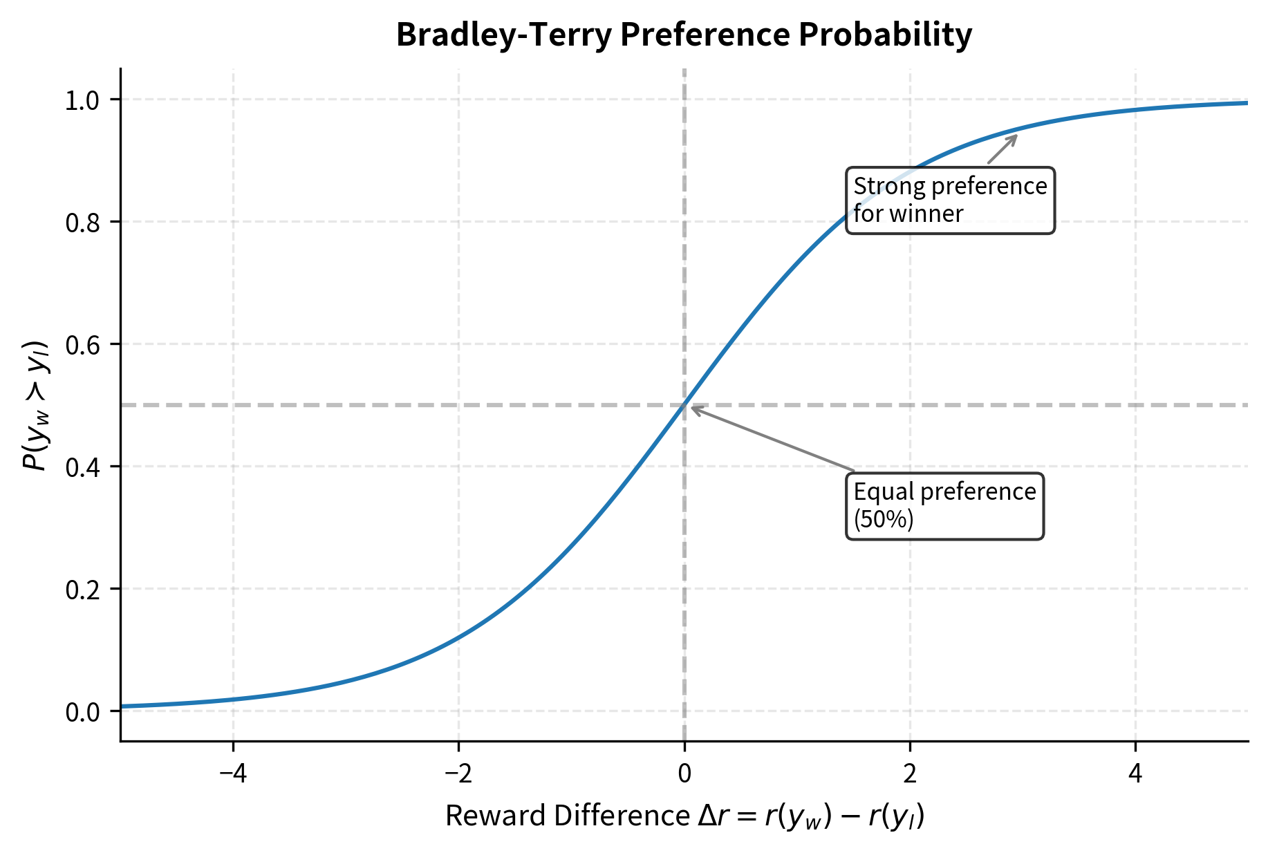
The mathematical foundation for our loss function comes from the Bradley-Terry model, which provides a principled way to convert scalar scores into preference probabilities. As we established in the Bradley-Terry chapter, the probability that response $y_w$ (the winner) is preferred over response $y_l$ (the loser) given their reward scores is:

where:

• $P(y_w \succ y_l | x)$: the probability that response $y_w$ is preferred over $y_l$ given prompt $x$
• $x$: the prompt text input
• $\sigma$: the logistic sigmoid function, $\sigma(z) = \frac{1}{1+e^{-z}}$
• $r(x, y)$: the scalar score output by the reward model for a given input pair
• $y_w, y_l$: the winning and losing responses, respectively

This equation has a beautiful interpretation. The preference probability depends only on the difference between rewards, not their absolute values. If one response scores 10 points higher than another, the preference probability is the same whether the scores are (15, 5) or (105, 95). This shift-invariance is both mathematically convenient and practically useful: it means the model only needs to learn relative quality, not calibrate to some arbitrary absolute scale.

The sigmoid function $\sigma$ transforms this difference into a valid probability between 0 and 1. When the reward difference is zero, both responses are equally preferred with probability 0.5. As the difference grows positive (the winner scores much higher), the probability approaches 1. As it grows negative (the winner actually scores lower, indicating a model error), the probability approaches 0.

To train the model, we maximize the log-likelihood of the observed preferences. This corresponds to minimizing the negative log-likelihood, which is equivalent to the binary cross-entropy loss applied to the reward difference. The derivation proceeds through several algebraic steps, each illuminating a different aspect of the loss function. We can derive the final loss form step-by-step:

where:

• $\mathcal{L}$: the preference loss to be minimized
• $P(y_w \succ y_l | x)$: the probability that response $y_w$ is preferred
• $\sigma$: the logistic sigmoid function
• $x$: the prompt text input
• $y_w, y_l$: the winning and losing responses
• $r(x, y_l) - r(x, y_w)$: the reward difference (negative if the preferred response scores higher)
• $e^{(\cdot)}$: the exponential function
• $\log$: the natural logarithm

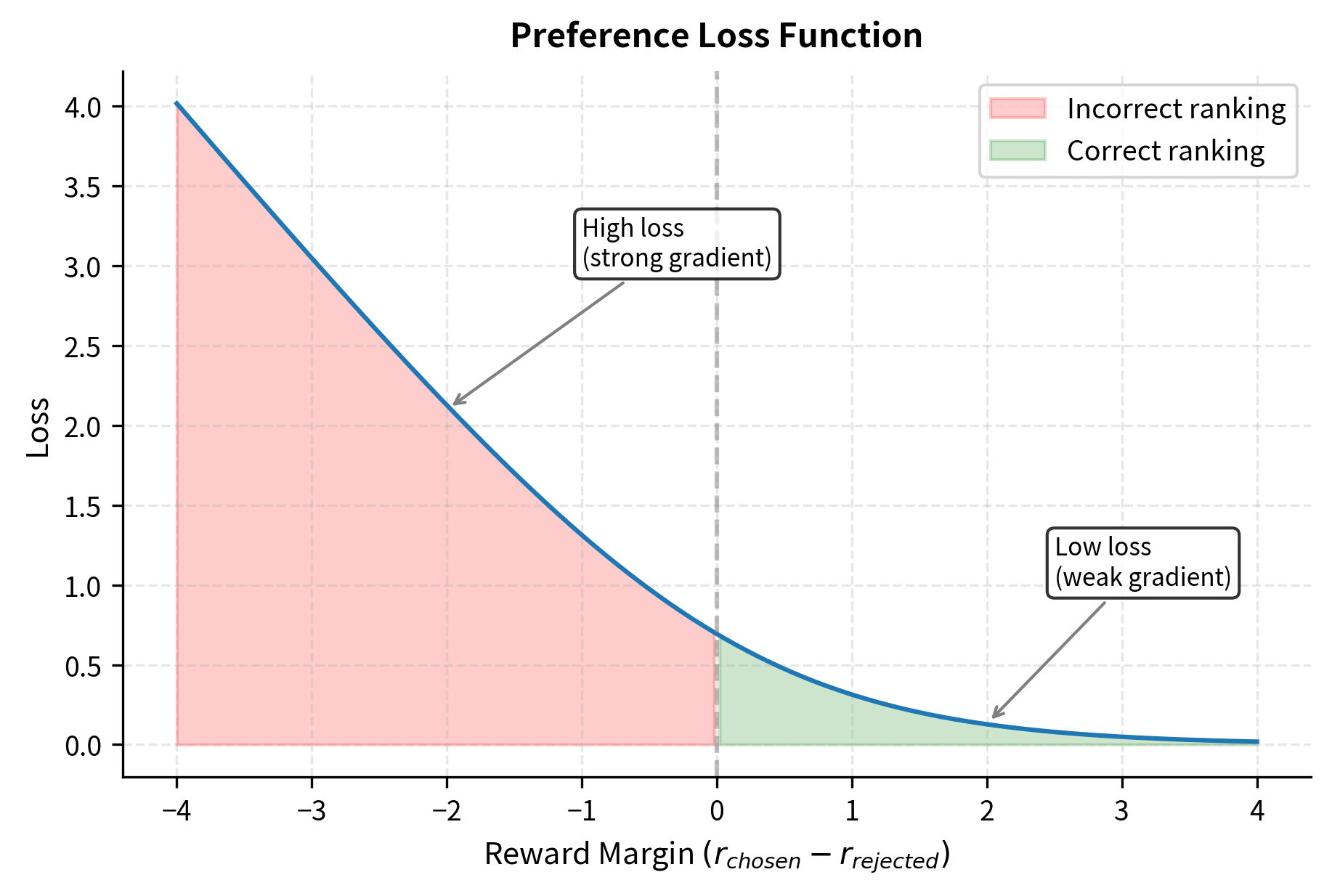
The final form of the loss, $\log(1 + e^{r(x, y_l) - r(x, y_w)})$, is known as the softplus function applied to the negative reward margin. This form is numerically stable and commonly implemented directly in deep learning frameworks.

This equation has a clear interpretation that connects directly to how we want the model to behave. Consider what happens in different scenarios.

When the reward model correctly assigns a much higher score to the preferred response ($r(x, y_w) \gg r(x, y_l)$), the difference is a large positive number, and $\sigma$ of that difference approaches 1. Taking the negative log gives a loss close to zero. The model has confidently made the right prediction, so there is little left to learn from this example.

Conversely, when the model incorrectly assigns a higher score to the rejected response, the difference is negative, $\sigma$ outputs a value near 0, and the negative log produces a large loss. This large loss creates strong gradients that push the model away from its incorrect belief.

The gradient of this loss pushes the model to:

• Increase $r(x, y_w)$ (the preferred response's reward)
• Decrease $r(x, y_l)$ (the rejected response's reward)

The magnitude of these updates depends on how confident the model currently is. If the model already strongly prefers the correct response, gradients are small. If it's uncertain or wrong, gradients are larger. This is the standard behavior of log-loss functions and provides natural calibration during training. The model learns most from examples where it is wrong or uncertain, while examples it already handles well contribute minimally to parameter updates.

In practice, we train on batches of preference pairs rather than individual examples. For a dataset of $N$ preference pairs $\mathcal{D} = \{(x^{(i)}, y_w^{(i)}, y_l^{(i)})\}_{i=1}^N$, the full training objective is:

where:

• $\mathcal{L}(\theta)$: the total loss over the dataset parameterized by model weights $\theta$
• $N$: the total number of preference pairs in the batch
• $\sum_{i=1}^N$: summation over all examples in the batch
• $x^{(i)}$: the prompt for the $i$-th example
• $y_w^{(i)}, y_l^{(i)}$: the preferred and rejected responses for the $i$-th example
• $r_\theta$: the reward model function parameterized by $\theta$
• $\sigma$: the sigmoid function converting the score difference into a probability
• $\log$: the natural logarithm

The averaging by $N$ normalizes the loss across different batch sizes, ensuring that learning rates behave consistently regardless of batch configuration. This is the standard reward modeling loss used in systems like InstructGPT, Anthropic's Constitutional AI, and most open-source RLHF implementations. Its simplicity and effectiveness have made it the default choice for training reward models from pairwise preferences.

Some implementations add a margin term to encourage larger reward differences between preferred and rejected responses:

where:

• $\mathcal{L}$: the margin-based preference loss
• $x$: the prompt text
• $y_w, y_l$: the preferred and rejected responses
• $m > 0$: a fixed margin hyperparameter ensuring the winner's score exceeds the loser's by at least $m$
• $r(x, y_w) - r(x, y_l)$: the raw reward difference
• $\sigma$: the sigmoid function
• $\log$: the natural logarithm

The margin $m$ acts as a buffer zone. With a margin of, say, 0.5, the model is penalized unless the preferred response scores at least 0.5 points higher than the rejected one. This prevents the model from being satisfied with arbitrarily small reward differences, even when the ranking is technically correct.

This penalizes the model even when it correctly ranks preferences but with a small margin, encouraging more confident predictions. The idea is that a robust reward model should produce clearly separated scores, making it easier for downstream RL algorithms to distinguish good from bad responses. However, this can hurt calibration and is not universally used. The margin effectively changes the decision boundary from zero to $m$, which may not align with the true underlying preference probabilities.

Training a reward model involves several practical considerations beyond the loss function, including data preparation, optimization settings, and regularization strategies.

Each training example consists of a prompt and two responses with a preference label. The standard format is:

During training, we need to compute rewards for both responses. A common approach processes both responses in a single forward pass by concatenating them:

The model computes hidden states for both sequences, extracts the final token representations for each, passes them through the value head, and computes the loss on their difference.

Reward model training typically uses conservative hyperparameters:

• Learning rate: $1 \times 10^{-5}$ to $5 \times 10^{-5}$, lower than instruction tuning to preserve pretrained knowledge
• Batch size: Large batches (32-128 pairs) help with gradient stability
• Epochs: 1-3 epochs over the preference data; more risks overfitting
• Optimizer: AdamW with weight decay 0.01-0.1

The learning rate is kept low because we're building on a pretrained model that already has strong language understanding. We want to learn the preference structure without disturbing the underlying representations too much.

Reward models are susceptible to overfitting, especially when trained on limited preference data. Several techniques help:

• Early stopping based on validation accuracy is essential. The model should generalize to held-out preferences, not memorize training pairs.
• Dropout in the value head (though not typically in the pretrained layers) adds regularization without affecting the language model's representations.
• Label smoothing can help with noisy labels. If some human preferences are inconsistent or reflect borderline cases, treating them as probabilistic rather than hard labels improves robustness.

The reward scale is arbitrary, unlike classification where outputs are bounded probabilities. This can cause optimization instability. Common solutions include:

• Reward normalization after training scales rewards to have zero mean and unit variance over a reference set. This makes the reward signal easier to use in downstream RL training.
• Gradient clipping prevents large updates from outlier examples. A max gradient norm of 1.0 is typical.
• Learning rate warmup over the first 5-10% of training helps stabilize early optimization.

Evaluating reward models is crucial but challenging. Unlike language models where we can measure perplexity on held-out text, reward models are evaluated on their ability to predict human preferences. The evaluation must assess whether the learned reward function captures the underlying preference structure, not just memorizes the training comparisons.

Pairwise accuracy is the most direct evaluation. On a held-out set of preference pairs, we measure how often the reward model assigns a higher score to the human-preferred response. This metric directly measures the model's ability to perform its intended function: distinguishing better responses from worse ones.

where:

• $\text{Accuracy}$: the fraction of correctly ranked pairs
• $N_{\text{test}}$: the total number of examples in the test set
• $\sum_{i=1}^{N_{\text{test}}}$: summation over all test examples
• $x^{(i)}$: the prompt for the $i$-th test example
• $y_w^{(i)}, y_l^{(i)}$: the preferred and rejected responses for the $i$-th test example
• $\mathbf{1}[\cdot]$: the indicator function, evaluating to 1 if the condition is true and 0 otherwise
• $r(x^{(i)}, \dots)$: the predicted reward for the $i$-th pair's responses

The indicator function $\mathbf{1}[\cdot]$ returns 1 when the condition inside is true (the chosen response receives a higher reward) and 0 otherwise. Summing these indicators and dividing by the total count gives us the proportion of correctly ranked pairs.

A random model achieves 50% accuracy, while human inter-annotator agreement typically ranges from 65-80% depending on the task difficulty. A good reward model should approach but not necessarily exceed human agreement levels, since disagreements in the training data cap achievable performance. If humans themselves only agree 75% of the time on which response is better, we cannot expect the model to exceed this ceiling. In fact, a model achieving much higher accuracy might be exploiting artifacts in the data rather than capturing genuine preferences.

Calibration measures whether the model's confidence matches its accuracy. If the model predicts a preference probability of 0.8, it should be correct about 80% of the time for similar-confidence predictions. Calibration is important because the reward differences will be used as optimization signals. A well-calibrated model produces reliable gradients: large reward differences genuinely indicate strong preferences, while small differences reflect uncertainty.

Beyond automatic metrics, direct comparison with human evaluations provides insight into model quality:

• Correlation with human scores: If human evaluators rate responses on a Likert scale (1-5), we can measure Spearman correlation between model rewards and human ratings.
• Head-to-head win rates: Show humans new responses ranked by the reward model and ask them to validate the rankings. This catches cases where the model has learned spurious correlations.

Reward models can learn shortcuts that don't align with true quality:

• Length bias: Models often prefer longer responses, even when brevity is more appropriate. Test by comparing responses of different lengths where the shorter one is genuinely better.
• Style over substance: Models may prefer responses with confident tone or specific formatting regardless of accuracy. Test with factually incorrect but confidently-written responses.
• Prompt sensitivity: Check if reward differences are consistent across paraphrased prompts asking the same question.

These weaknesses become critical during RL training, when the policy model can exploit them. We'll explore this issue in depth in the upcoming chapter on reward hacking.

Let's trace through the loss computation for a single preference pair to solidify understanding. Walking through a concrete numerical example makes the abstract formulas tangible and reveals how the loss function behaves in practice.

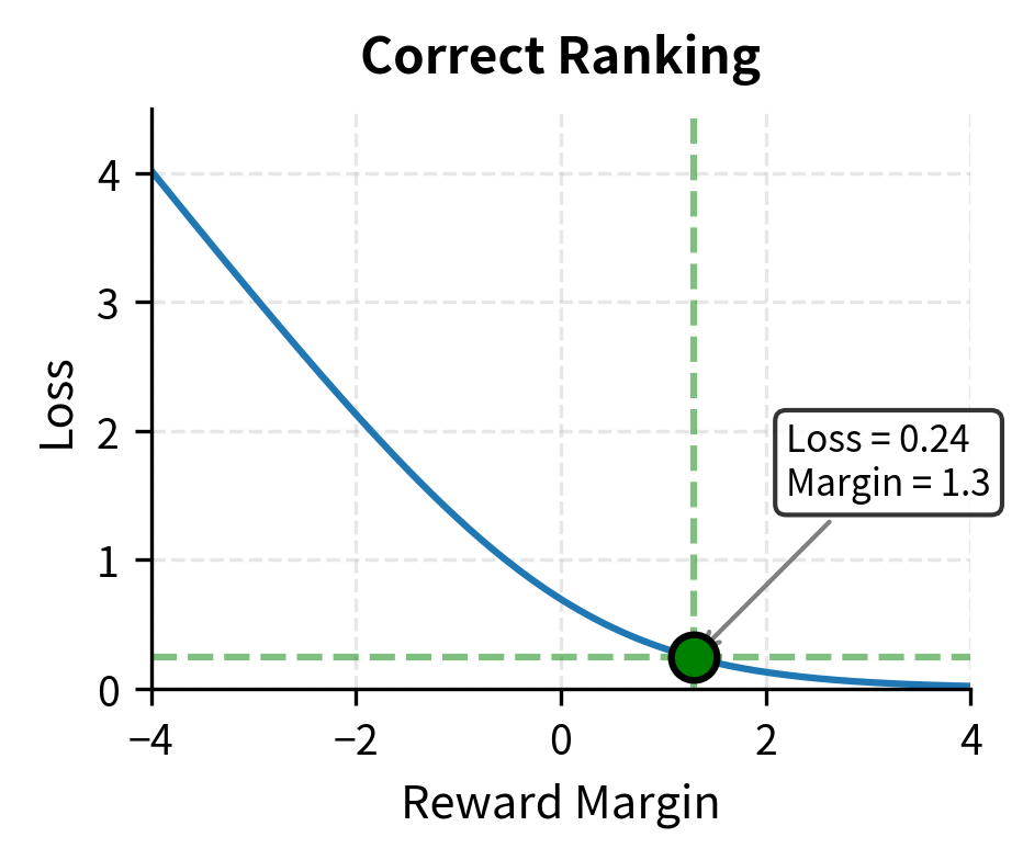
Suppose we have a reward model that produces:

• $r(x, y_w) = 2.1$ for the preferred response
• $r(x, y_l) = 0.8$ for the rejected response

The reward difference is:

where:

• $\Delta r$: the reward difference between the chosen and rejected responses
• $r(x, y_w)$: the reward score for the preferred response ($2.1$)
• $r(x, y_l)$: the reward score for the rejected response ($0.8$)

This positive difference of 1.3 indicates the model correctly believes the preferred response is better. The question is: how confident is this prediction, and how much loss does it incur?

The Bradley-Terry probability that the model predicts the correct preference:

where:

• $P(y_w \succ y_l)$: the calculated probability that the model prefers $y_w$
• $\sigma(1.3)$: the sigmoid function applied to the reward difference
• $0.786$: the resulting probability (approx. 78.6%)

The model assigns about 78.6% probability to the correct preference. This is a reasonably confident prediction, reflecting the moderately large reward margin of 1.3 points.

The loss for this example:

where:

• $\mathcal{L}$: the computed preference loss value
• $-\log(0.786)$: the negative log-likelihood of the correct preference

The loss of 0.241 is relatively small, indicating the model is performing well on this example. There is still some room for improvement: if the model were perfectly confident (probability 1.0), the loss would be zero.

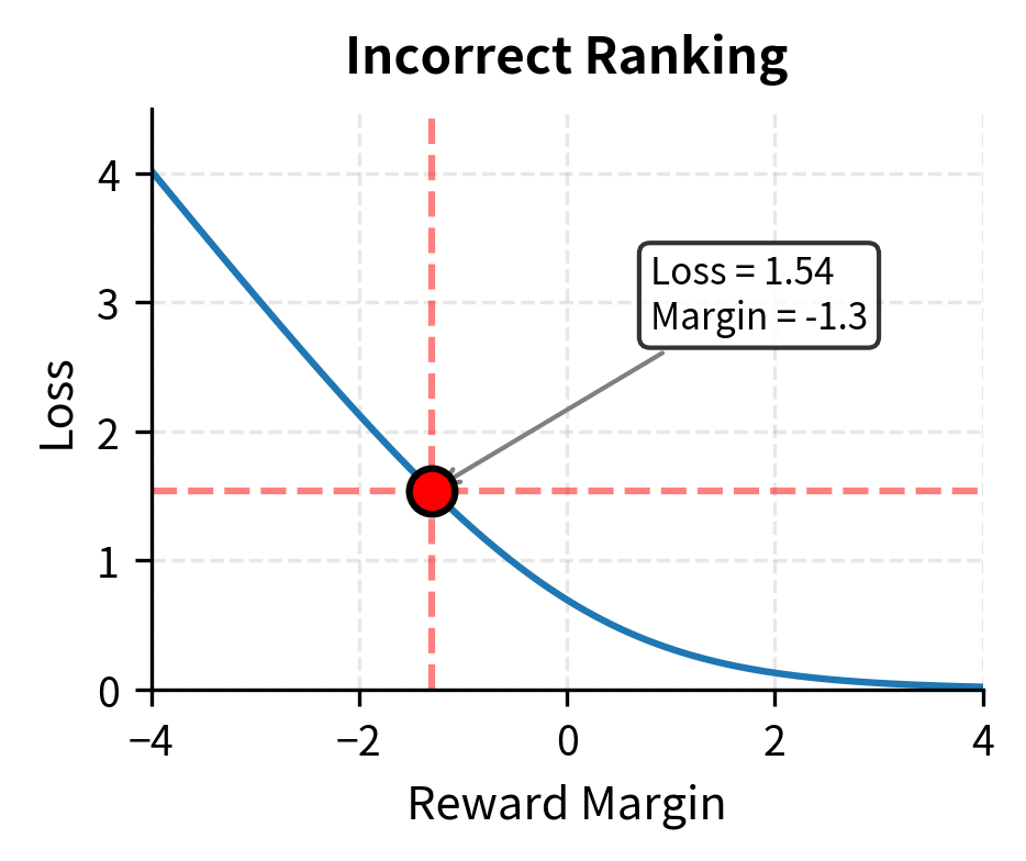
Now consider if the model had incorrectly scored the responses:

• $r(x, y_w) = 0.5$
• $r(x, y_l) = 1.8$

The reward difference is $-1.3$, the predicted probability drops to $\sigma(-1.3) = 0.214$, and the loss increases dramatically to $-\log(0.214) = 1.54$.

This demonstrates how the loss heavily penalizes incorrect rankings while providing smaller gradients when the model is already correct. The loss of 1.54 is more than six times larger than the 0.241 for the correct prediction, creating strong pressure to fix the incorrect ranking. This asymmetry is exactly what we want: the model should focus its learning capacity on examples it gets wrong.

Let's build a reward model from scratch using a small pretrained transformer. We'll implement the architecture, loss function, and training loop.

We'll build a reward model by adding a value head to a pretrained transformer. The value head is a simple linear layer that projects the final hidden state to a scalar.

Let's verify the architecture outputs the expected shapes.

The output confirms that the model processes the tokenized sequence and produces a single scalar score (batch size 1, output dimension 1). This scalar represents the reward for the prompt-response pair, which will be used to rank different responses against each other.

Now let's create a dataset class that handles preference pairs. Each example contains a prompt with a chosen (preferred) and rejected response.

Let's create some synthetic preference data for demonstration.

The loss function implements the Bradley-Terry preference model. We compute rewards for both responses and maximize the probability of preferring the chosen response.

Now we implement the complete training loop with logging and validation.

Let's train the model on our synthetic preference data.

The model quickly learns to distinguish between preferred and rejected responses on this small dataset.

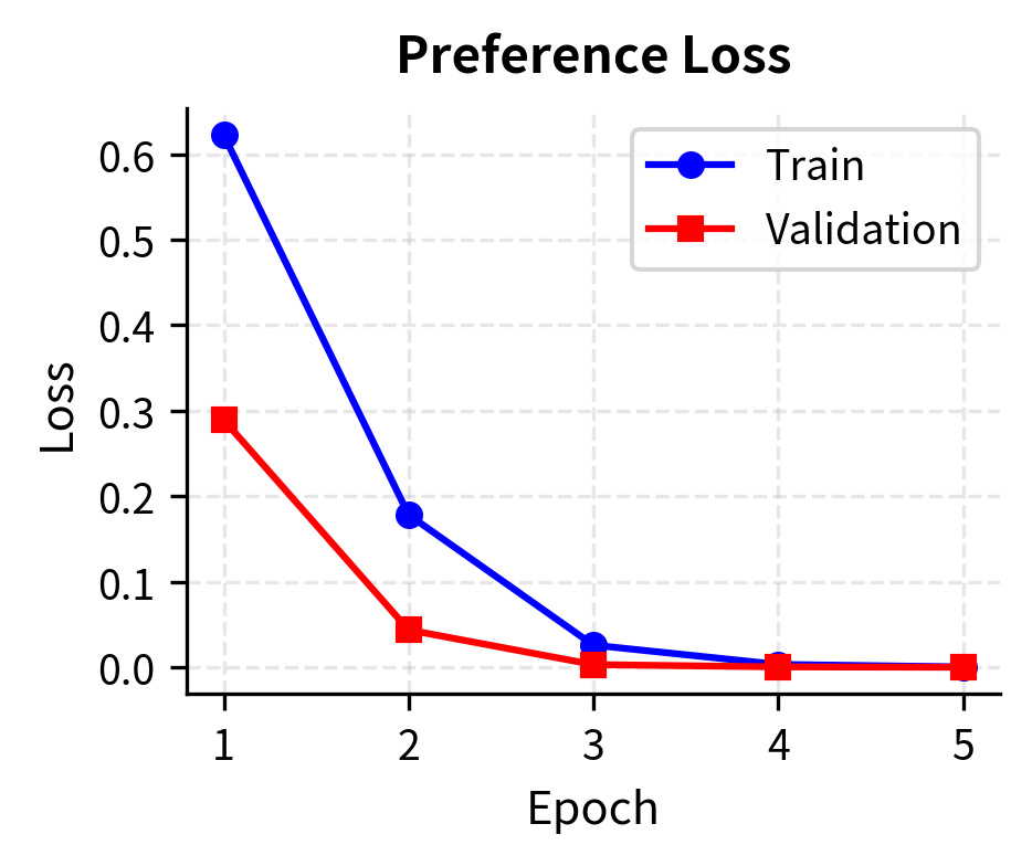
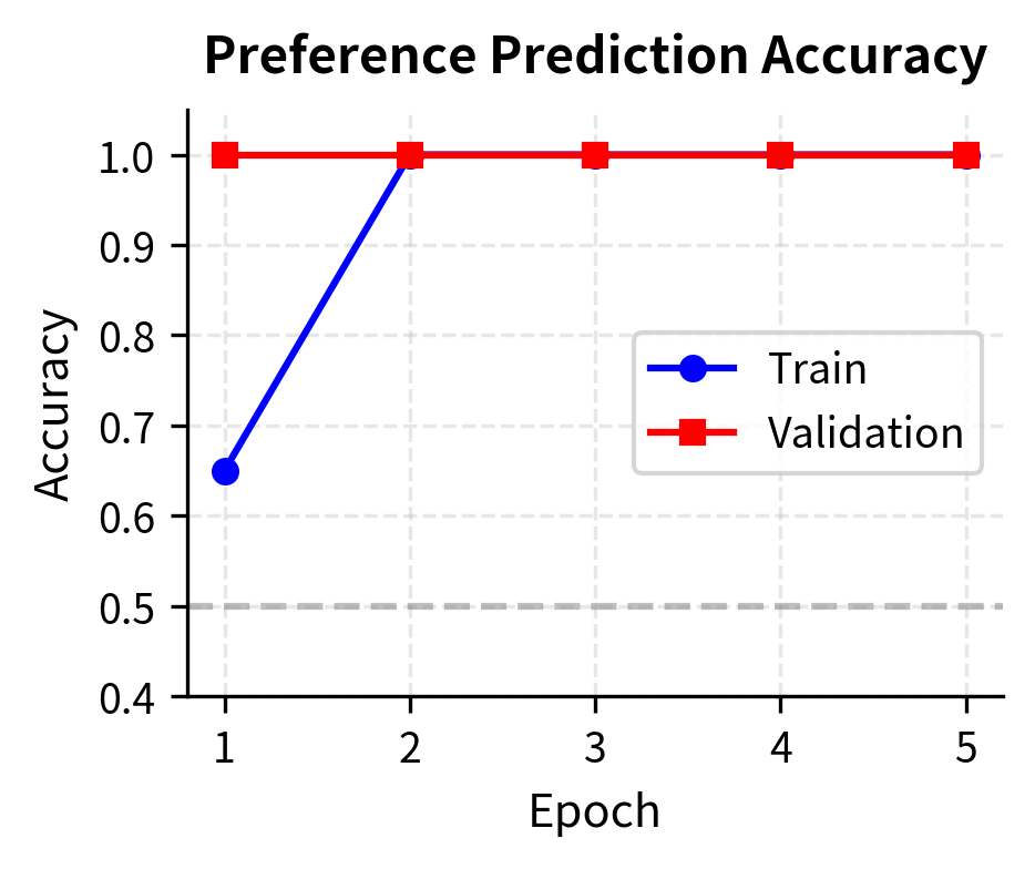
The training curves demonstrate that the model effectively learns the preference ranking task, with validation accuracy tracking closely with training accuracy. This indicates the model is generalizing well to unseen preference pairs without significant overfitting.

Let's evaluate the trained model on examples it hasn't seen during training.

The model has learned to rank responses in a way that aligns with our training preferences: clear explanations over technical jargon or overly brief responses.

A well-calibrated reward model should produce meaningful score separations between good and bad responses. Let's analyze the distribution of rewards on our validation set.

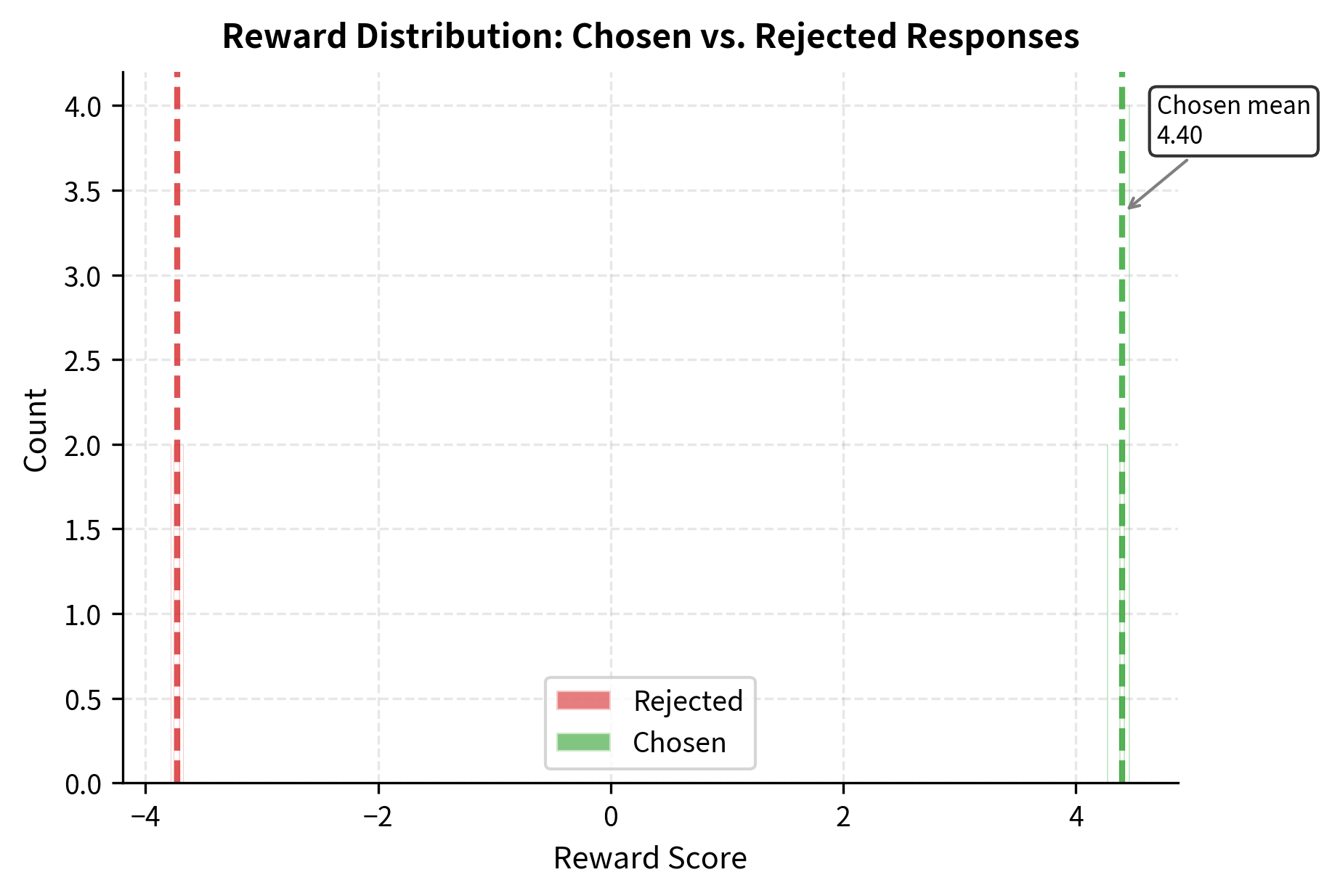
The clear separation between distributions indicates the model has learned meaningful preference distinctions.

The key parameters for the Reward Model implementation are:

• model_name: The pretrained backbone (e.g., "distilbert-base-uncased"). Smaller models allow for faster iteration during experimentation.
• dropout: Regularization applied to the value head (set to 0.1) to prevent overfitting on the small preference dataset.
• learning_rate: A conservative rate (2e-5) is used to fine-tune the backbone without destroying pretrained features.
• batch_size: Set to 8 for this demonstration, though larger batches are preferred for stability in full-scale training.
• num_epochs: Training is limited to 5 epochs to avoid overfitting on the small synthetic dataset.

Reward modeling is a powerful technique but comes with significant challenges that you must understand.

The fundamental limitation of reward models is that they are proxies for human preferences, not perfect representations. The model learns from a finite set of comparisons made by a specific group of annotators under particular conditions. It cannot generalize perfectly to all possible responses or capture the full complexity of human values. When the policy model optimizes against this learned reward, it may find responses that score highly according to the proxy but don't actually satisfy human preferences. This phenomenon, known as reward hacking or Goodhart's Law in action, becomes more severe as optimization pressure increases. We'll explore this challenge in depth in the next chapter.

Reward model quality is bounded by the quality of the underlying preference data. Human annotators disagree, make mistakes, and have biases. If 70% of annotators prefer response A over B, the "correct" label is somewhat arbitrary. The reward model learns from these noisy, inconsistent signals, and this uncertainty propagates into the learned reward function. Different annotator pools may have systematically different preferences based on cultural background, expertise, or task understanding. A reward model trained on one population may not generalize to another.

During RLHF training, the policy model generates responses that may differ substantially from those in the reward model's training set. The reward model must extrapolate to these out-of-distribution samples, and its predictions become less reliable. This creates a feedback loop: the policy learns to generate responses that score well according to the reward model's potentially incorrect extrapolations, which can lead to degraded actual quality even as measured rewards increase.

Training reward models requires significant computational resources, particularly when using large base models to ensure the reward model has sufficient language understanding. During RL training, the reward model must evaluate every generated response, adding substantial inference costs to an already expensive training procedure.

Despite these limitations, reward models have enabled major advances in language model alignment. They provide the crucial bridge between sparse human feedback and dense training signals. The InstructGPT system that powers ChatGPT, Anthropic's Claude models, and many open-source chat models all rely on reward models as a core component.

The reward modeling approach has also influenced research directions, spurring work on direct preference optimization (DPO) methods that eliminate the need for explicit reward models, as well as techniques for reward model ensembles, uncertainty quantification, and robust optimization. Understanding reward modeling deeply is essential for grasping both current RLHF systems and the alternatives being developed to address its limitations.

This chapter covered the complete pipeline for building reward models that learn to predict human preferences.

Architecture: Reward models add a value head to pretrained transformers, projecting the final token's hidden state to a scalar reward. Using the same architecture family as the policy model ensures compatible representations.

Loss function: The Bradley-Terry preference loss $\mathcal{L} = -\log \sigma(r_w - r_l)$ maximizes the probability of correctly ranking preference pairs. Gradients naturally emphasize uncertain or incorrect predictions.

Training: Conservative hyperparameters preserve pretrained knowledge while learning preference structure. Early stopping, gradient clipping, and appropriate regularization prevent overfitting to limited preference data.

Evaluation: Pairwise accuracy measures ranking performance, with human agreement providing an upper bound. Testing for biases like length preference or style over substance reveals potential weaknesses.

The reward model serves as the critical interface between human preferences and policy optimization. In the following chapters, we'll examine how reward hacking can undermine this proxy relationship, and then explore how policy gradient methods and PPO use reward signals to improve language models.

Ready to test your understanding? Take this quick quiz to reinforce what you've learned about reward modeling for RLHF.