

Master Hierarchical Navigable Small World (HNSW) graphs for vector search. Learn graph architecture, construction, and tuning for high-speed retrieval.

This article is part of the free-to-read Language AI Handbook
Choose your expertise level to adjust how many terms are explained. Beginners see more tooltips, experts see fewer to maintain reading flow. Hover over underlined terms for instant definitions.
execute: cache: true jupyter: python3
HNSW Index
In the previous chapter, we explored vector similarity search and the fundamental challenge it presents: given a query vector, find the most similar vectors in a collection. The brute-force approach, computing distances between the query and every vector in the database, delivers perfect accuracy but scales linearly with the number of vectors. For a million-document corpus with 768-dimensional embeddings, every single query requires a million high-dimensional distance computations. For ten million documents, it requires ten million. This quickly becomes impractical for the real-time retrieval that RAG systems demand.
Approximate nearest neighbor (ANN) search addresses this scalability issue. Rather than guaranteeing exact nearest neighbors, ANN algorithms trade a small amount of accuracy for dramatic speed improvements, often returning results in milliseconds even across billion-vector collections. Among the many ANN algorithms developed over the years, one has emerged as the dominant choice for vector search in production systems: Hierarchical Navigable Small World graphs, or HNSW.
HNSW, introduced by Yuri Malkov and Dmitry Yashunin in 2016, combines two powerful ideas: the "small world" property of certain graphs (where any node can reach any other node in surprisingly few hops) and a hierarchical layering scheme inspired by skip lists. The result is an index structure that supports both fast construction and fast search, with tunable parameters that let you precisely control the tradeoff between speed and recall. HNSW powers the vector search behind libraries like FAISS, Hnswlib, and vector databases such as Pinecone, Weaviate, Qdrant, and Milvus.
Small World Graphs
To understand HNSW, we need to start with the concept that gives it half its name: small world graphs.
In the 1960s, psychologist Stanley Milgram conducted his famous "small world" experiment, asking people to forward letters to a target person through chains of acquaintances. He found that most letters arrived in about six steps, giving rise to the popular phrase "six degrees of separation." This phenomenon, where nodes in a large network can reach each other through surprisingly short paths, is the small world property.
A graph exhibits the small world property when the average shortest path between any two nodes grows logarithmically (or slower) with the number of nodes. In a graph with nodes, the average path length scales as rather than .
To appreciate why this property is remarkable, consider the contrast with what we might naively expect. If a graph has a million nodes and each node connects only to a few neighbors, you might imagine that traversing from one side of the graph to the other would require thousands or even hundreds of thousands of hops. In a chain or grid structure, that intuition holds true: the number of hops scales with the diameter of the structure, which can be proportional to or . But small world graphs defy this expectation. Even as the number of nodes grows into the millions or billions, the average path length between any two nodes increases only logarithmically.
What makes social networks "small worlds" is the combination of two structural features:
- Local clustering: People tend to know others in their immediate community, creating dense local neighborhoods. Your friends are likely friends with each other, forming tightly knit clusters of mutual connections.
- Long-range connections: A few connections bridge distant communities (a friend who moved abroad, a colleague in a different industry), providing shortcuts across the graph. These rare but critical links act as express highways, allowing you to jump from one cluster to a completely different one in a single step.
The interplay between these two features creates the small world property. Local clustering alone would produce a graph where short paths exist only within communities, and reaching a distant community would require traversing the entire structure. Long-range connections alone would create a graph where you can jump anywhere quickly but lack the dense local structure needed for precise navigation once you are in the right neighborhood. Together, they enable a style of traversal where long-range hops bring you close to your target quickly, and then dense local connections let you zero in on exactly the right node.
This same structure turns out to be incredibly useful for nearest neighbor search. If we build a graph where vectors are nodes and edges connect similar vectors, we can navigate from any starting point to any query's nearest neighbor by repeatedly jumping to the most promising neighbor, much like forwarding Milgram's letters. The key realization is that vector similarity naturally provides the notion of "closeness" needed to organize these connections: nearby vectors in the embedding space form the local clusters, while occasional connections to more distant vectors serve as the long-range bridges.
Navigable Small World Graphs
A small world graph guarantees that short paths exist between any two nodes, but that alone isn't enough. We also need to be able to find those short paths efficiently, without knowing the global structure of the graph. This introduces navigability, a subtle but critical distinction.
The existence of a short path is a property of the graph's topology. Navigability, by contrast, is a property of how easily a simple, local algorithm can discover and follow that path. Imagine being dropped into a massive city with no map. Knowing that every location is reachable within a few blocks is reassuring, but useless if you have no way to decide which direction to walk at each intersection. Navigability means that at every intersection, looking only at the streets immediately available to you, you can make a locally informed decision that consistently brings you closer to your destination.
A graph is navigable if a greedy routing algorithm, one that always moves to the neighbor closest to the target, can efficiently find short paths between any pair of nodes. The key insight is that routing decisions are made using only local information (the current node's neighbors), not global knowledge of the graph.
Consider a simple greedy search on such a graph. You start at some entry node and want to reach the node closest to your query vector . At each step, you look at all neighbors of your current node, compute their distances to , and move to whichever neighbor is closest. You stop when no neighbor is closer to than your current node. This is a classic greedy best-first search, and its elegance lies in its simplicity: no priority queues spanning the entire graph, no global routing tables, and no precomputed shortest paths. The only information the algorithm uses at each step is the set of neighbors of the current node and their distances to the query.
For this to work well, the graph needs those same two structural ingredients we discussed above, but now viewed through the lens of routing. Dense local connections ensure that once you are near the target, you can find it precisely. Without them, the greedy search might reach the right neighborhood but be unable to take the final steps to the exact nearest neighbor, because no edge connects the current node to the true answer. Long-range connections ensure that you can quickly traverse from distant regions of the vector space to the target's neighborhood. Without them, the greedy search would have to take many small steps, inching across the space one local cluster at a time, turning what should be a logarithmic traversal into a linear one.
The problem with a flat (single-layer) NSW graph is that the greedy search can get trapped. As the graph grows, long-range connections become increasingly diluted by short-range ones. Early in the search, when you're far from the target, you need long-range jumps to make progress quickly. But in a large flat graph, the probability of finding a useful long-range connection among a node's fixed-size neighbor list diminishes. Consider what happens during graph construction: when a node is inserted, its neighbors are chosen from the closest existing nodes. In a large graph, those closest nodes are very nearby, so the resulting edges are short-range. Long-range edges, which were created early when the graph was small and "closest" meant "relatively far away," become a smaller and smaller fraction of the total edges. The search degrades, requiring more hops and more distance computations, and the greedy algorithm's performance begins to approach the very linear scaling we are trying to avoid.
The Hierarchical Insight
HNSW solves the long-range navigation problem with an elegant idea borrowed from skip lists, a probabilistic data structure for sorted sequences.
In a skip list, elements exist on multiple levels. The bottom level contains all elements. Each higher level contains a random subset of the elements from the level below, with roughly half as many elements per level. Searching starts at the top level, where elements are sparse and each hop covers a large range, then descends to lower levels for finer-grained search. This gives search time. A skip list achieves the efficiency of a balanced binary search tree without requiring complex rebalancing operations, relying instead on simple randomization to maintain its structure.
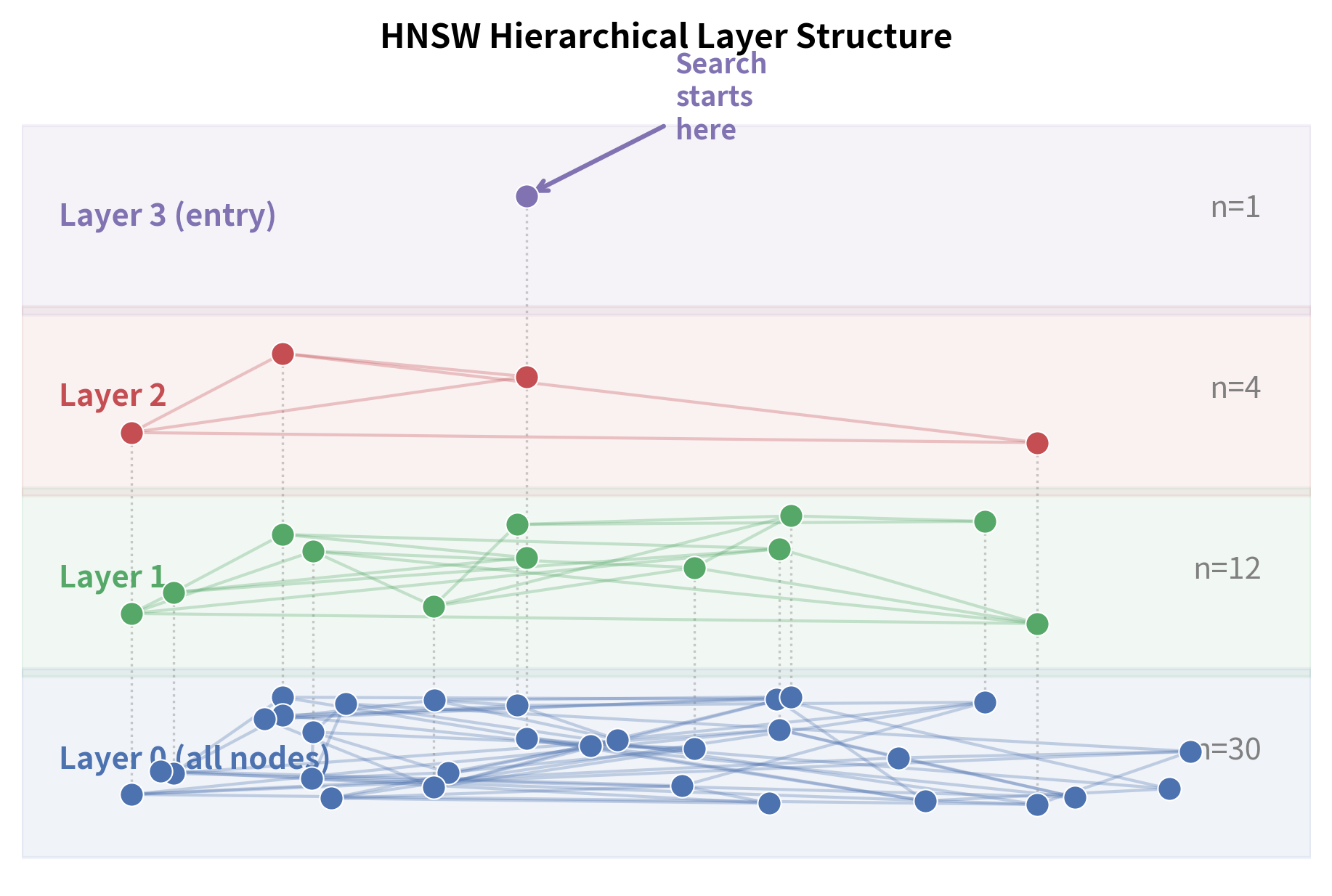
HNSW applies the same principle to graph-based nearest neighbor search, translating the one-dimensional skip list into a multi-dimensional navigable graph hierarchy. Instead of a single graph, HNSW builds a hierarchy of graphs across multiple layers:
- Layer 0 (the bottom layer) contains all vectors, connected to their nearest neighbors with short-range edges. This layer is the most densely populated and provides the fine-grained resolution needed to identify the true nearest neighbors.
- Layer 1 contains a subset of vectors, connected with edges that naturally span longer distances (because the nodes are more spread out). Since fewer nodes exist on this layer, even connecting to "nearest neighbors" produces edges that cover more ground in the vector space.
- Layer 2 contains an even smaller subset, with even longer-range connections. The sparser the layer, the more each edge acts as a highway through the space.
- The top layer contains just a handful of nodes, providing a coarse "highway" across the entire vector space. A single hop on this layer might span a distance that would require dozens of hops on layer 0.
HNSW determines which layer each node belongs to using a randomized assignment process that mirrors the probabilistic structure of skip lists. Each node is assigned a maximum layer using a random process. Most nodes exist only on layer 0. Fewer nodes reach layer 1, fewer still reach layer 2, and so on. The maximum layer is assigned using a formula that ensures this exponential decay:
We examine each component and its role in producing the desired distribution of layers:
- : the maximum layer assigned to the node. A node assigned layer will exist on every layer from 0 up to , meaning it participates in the graph at multiple levels of the hierarchy.
- : a random value drawn from a uniform distribution between 0 and 1. This is the source of randomness that ensures different nodes end up on different layers. Each insertion draws independently from this distribution.
- : this transformation is a classic technique known as inverse transform sampling. The negative natural logarithm of a uniform random variable produces a value that follows an exponential distribution with rate parameter 1. Most of the time, the uniform draw is close to 1, making close to 0, which means most nodes will be assigned to low layers. Occasionally, the uniform draw is close to 0, producing a large value of and placing the node on a high layer. This naturally produces the "many nodes at the bottom, few at the top" structure we need.
- : the level multiplier, typically set to . This scaling factor controls how quickly the exponential distribution decays and, consequently, how many nodes appear on each successive layer. By tying to , the formula ensures that the probability of reaching layer is proportional to . In other words, each layer has roughly times as many nodes as the layer below it.
- : the floor function, which discretizes the continuous exponential value into integer layers. Since layers are discrete (layer 0, 1, 2, ...), the continuous value must be rounded down to the nearest integer.
The net effect of this formula is that each layer has roughly times as many nodes as the layer below, mirroring the skip list structure. This exponential thinning is what gives HNSW its logarithmic search complexity: the number of layers grows as , and each layer requires only a bounded number of greedy steps, so the total search cost scales logarithmically with the number of vectors.
This design naturally separates the two phases of search:
- Coarse navigation (upper layers): With few, widely-spaced nodes, each greedy step covers a large distance. You quickly zoom into the right region of the space. Because the nodes on upper layers are sparse representatives of the entire collection, the graph on each upper layer acts like a coarse map, and greedy routing on this map efficiently narrows the search to the correct neighborhood.
- Fine-grained search (lower layers): With many densely-connected nodes, you refine your search to find the actual nearest neighbors. Once the upper layers have brought you to approximately the right region, layer 0's dense connectivity ensures that the final, precise answer is reachable within a few more hops.
Graph Construction
HNSW builds its index incrementally: vectors are inserted one at a time, and each insertion both places the new node into the graph and establishes connections to existing nodes. This incremental approach means the graph evolves as data is added, with each new vector benefiting from the structure already in place and simultaneously enriching that structure for future insertions. The construction algorithm has two main phases for each inserted element.
Assigning a Layer
When a new element is inserted, the first decision the algorithm must make is which layers this element will inhabit. This is determined by assigning a maximum layer using the randomized formula:
As we discussed in the previous section, this formula transforms a uniform random draw into a geometrically decaying layer assignment. Let us revisit each component briefly in the context of construction:
- : the maximum layer assigned to the node. The element will be present on every layer from 0 through , and edges will be created for it on each of these layers.
- : a random value drawn from a uniform distribution between 0 and 1. This is drawn independently for each inserted element, ensuring that the layer assignments are uncorrelated.
- : a transformation using inverse transform sampling to convert the uniform value into an exponential distribution. Because the exponential distribution is heavily concentrated near zero, most nodes receive small values, and consequently low layer assignments.
- : the level multiplier (typically ), which scales the distribution to control the decay rate of layer probabilities. The choice of ties the layer structure directly to the connectivity parameter , ensuring that the hierarchy has the right density at each level.
- : the floor function, which discretizes the continuous value into integer layers, since the hierarchy consists of discrete levels numbered 0, 1, 2, and so on.
This formula produces an exponential distribution of layers. With and , the probabilities work out roughly as:
- ~94% of nodes exist only on layer 0
- ~6% reach layer 1
- ~0.4% reach layer 2
- Negligible fraction reach layer 3 or higher
These numbers convey an important structural insight: the vast majority of nodes live only on the bottom layer, where they contribute to the dense, fine-grained connectivity needed for precise nearest neighbor identification. A small fraction of nodes are "promoted" to higher layers, where they serve as landmarks and waypoints for long-range navigation. And only a tiny handful reach the topmost layers, where they act as universal entry points from which any search can begin. This exponential decay is precisely what creates the skip list-like structure. Each layer is roughly times sparser than the one below it.
Finding Neighbors for Connection
Once the new element has its assigned layer , the algorithm needs to find good neighbors to connect it to on each layer from down to 0. The quality of these connections is critical: they determine whether the graph will be navigable and whether future searches will be able to efficiently route through this part of the space. This happens in two phases:
Phase 1: Descend to the insertion layer. Starting from the global entry point at the top layer, perform a simple greedy search (beam width of 1) on each layer above . At each layer, walk greedily toward until no closer neighbor can be found, then descend. This phase simply navigates to a good starting point for the actual insertion work. No connections are made during this descent. The purpose is purely navigational: by the time the algorithm reaches layer , it has identified a node that is reasonably close to in the vector space, providing a high-quality starting point for the neighbor search that follows.
Phase 2: Insert and connect. Starting from layer down to layer 0, perform a broader search (with beam width ef_construction) to find the closest existing nodes to . The parameter ef_construction governs how thoroughly the algorithm explores the neighborhood around . A larger ef_construction means more candidate nodes are examined, increasing the likelihood of finding the truly best neighbors at the cost of additional distance computations. From these candidates, select the best neighbors and create bidirectional edges between and each selected neighbor. The bidirectionality is essential: it ensures that is not only reachable from its neighbors, but that 's neighbors are also reachable from , maintaining the graph's navigability in both directions.
The selection of which neighbors to connect is critical and deserves careful attention. The simplest approach is to pick the closest nodes, but HNSW uses a more sophisticated heuristic that favors diversity. The heuristic prefers neighbors that are not only close to but also cover different "directions" in the vector space. This prevents all connections from clustering in one region and ensures better navigability.
To understand why diversity matters, imagine a scenario where a new node is positioned at the edge of a dense cluster. The closest nodes might all be members of that same cluster, all lying in roughly the same direction from . If connects only to these nearby cluster members, there would be no edge leading outward from toward other regions of the space. Future searches passing through would find it easy to reach the nearby cluster but impossible to exit toward other clusters. The diversity heuristic avoids this trap by ensuring that connections reach outward in multiple directions.
The neighbor selection heuristic works as follows. Candidates are sorted by distance to . For each candidate (in order of increasing distance), is added to the neighbor set only if it is closer to than it is to any already-selected neighbor. In other words, a candidate is rejected if it is "covered" by an already-chosen neighbor:
We define the meaning and purpose of each symbol in this condition:
- : the candidate neighbor being considered. Candidates are examined one at a time, in order of increasing distance from , so the closest candidates are considered first.
- : the newly inserted element, the node for which we are selecting neighbors.
- : the distance between and , measured using whatever metric the index employs (Euclidean, inner product, or cosine distance).
- : the set of neighbors already chosen for . This set starts empty and grows as candidates pass the heuristic test.
- : the distance from the candidate to the closest already-selected neighbor. This is the crux of the heuristic. If is very close to some already-selected neighbor , then already "covers" the direction that would provide. Adding would be redundant, as searches arriving at could reach 's region of the space by going through instead.
This condition ensures that we only add if it is closer to than to any existing neighbor. The geometric intuition is that each selected neighbor "claims" a region of space around it, and a new candidate is accepted only if it lies in an unclaimed direction. This encourages connections that spread outward in different directions, creating the diverse connectivity that makes the graph navigable. The result is a neighbor list where each connection opens up a distinct corridor through the vector space, maximizing the routing options available to future searches passing through .
Handling Overflow
When a new edge is added between and an existing node , the node might end up with more than connections. This overflow can happen because the bidirectional edge creation means that receives a new neighbor even though 's original neighbor list was already full. In this case, 's neighbor list is pruned back to using the same heuristic selection described above, keeping the most useful connections and discarding redundant ones. The pruning re-evaluates all of 's current neighbors (including the newly added ) and retains the set that best satisfies the diversity criterion, ensuring that 's connections continue to cover multiple directions. The paper uses for layers above 0, and for layer 0, since the bottom layer benefits from denser connectivity. The rationale for doubling the connection limit on layer 0 is that this is where the most precise search occurs, and having more edges per node increases the probability that the greedy search can reach the exact nearest neighbor without getting stuck in a local minimum.
Construction Algorithm Summary
The full construction algorithm for inserting element :
- Assign random layer to
- Set entry point to the current graph's entry point
- For each layer from the top down to : greedily search for the nearest node to , update
- For each layer from down to 0:
a. Search for
ef_constructionnearest candidates to starting from b. Select up to neighbors from candidates using the heuristic c. Add bidirectional edges between and selected neighbors d. For any neighbor that now exceeds connections, prune its neighbor list - If is higher than the current maximum layer, update the entry point to
Step 5 deserves a brief note: whenever a newly inserted node reaches a layer higher than any existing node, it becomes the new global entry point for the entire index. This ensures that searches always begin at the topmost layer, where the sparsest, most globally connected node provides the starting point for the coarse navigation phase.
Search Procedure
Searching an HNSW index follows the same two-phase pattern as construction, but optimized for finding the nearest neighbors of a query vector . The search algorithm leverages the hierarchical structure to decompose the problem into a fast coarse approach followed by a thorough local exploration, and this decomposition is what gives HNSW its characteristic efficiency.
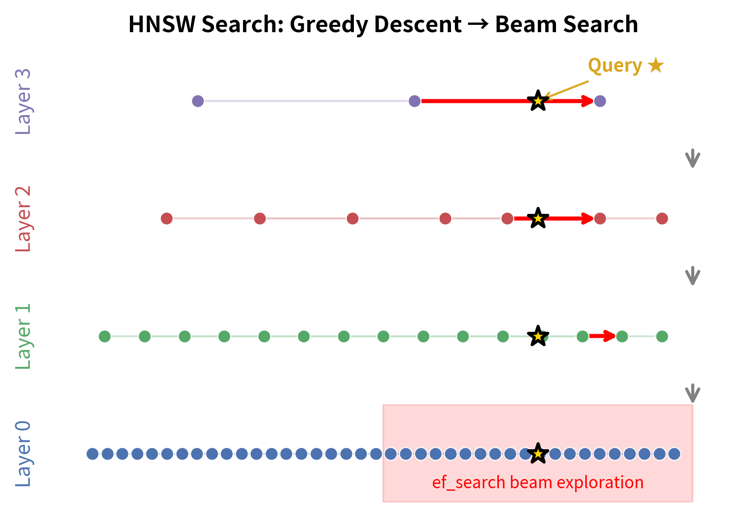
Phase 1: Greedy Descent Through Upper Layers
Starting from the entry point on the top layer, perform a simple greedy search with beam width 1. At each layer, repeatedly move to the neighbor closest to until no improvement is possible. Then descend to the next layer, using the current best node as the entry point for the layer below.
This phase is fast because upper layers are sparse. Each greedy step on the top layer might skip over millions of vectors in a single hop. The descent quickly narrows the search to the right neighborhood. To build a concrete intuition, consider a graph with 10 million vectors and . The top layer might contain only a handful of nodes, and a single greedy step on this layer could jump from one end of the vector space to the other. Layer 2 might contain a few thousand nodes, and each hop covers a correspondingly smaller but still substantial distance. By the time the algorithm reaches layer 1, it has narrowed the search region from the entire collection down to a small neighborhood containing perhaps a few thousand nearby vectors. The total number of distance computations during this descent is remarkably small, typically just a few per layer, because only a single candidate (the current best) is tracked.
Phase 2: Beam Search on Layer 0
Once you reach layer 0, the algorithm switches strategy. The greedy descent with beam width 1 was efficient but coarse; it found a good starting neighborhood but may not have identified the exact nearest neighbors. Layer 0, which contains all vectors, is where the precise answer lives. To find it, the algorithm performs a more thorough search using a beam width of ef_search (where ef_search ). This is essentially a best-first search that maintains a dynamic candidate list:
- Initialize a candidate set and a result set with the entry point from Phase 1.
- While is not empty:
a. Extract the nearest unvisited candidate from
b. If is farther from than the farthest element in , stop (no more useful candidates)
c. For each neighbor of that hasn't been visited:
- If is closer to than the farthest element in (or
ef_search), add to both and - If
ef_search, remove the farthest element from
- If is closer to than the farthest element in (or
- Return the closest elements from
The stopping condition in step 2b is the key to this algorithm's efficiency: the moment the best remaining candidate is worse than the worst element already in the result set, the search terminates. This means the algorithm does not exhaustively explore all reachable nodes; instead, it expands outward from the entry point in order of proximity to the query, and stops as soon as further expansion cannot possibly improve the results.
The parameter ef_search controls how thorough this search is. A larger ef_search explores more candidates, improving recall at the cost of more distance computations. Setting ef_search = k gives the fastest (but least accurate) search, while larger values progressively improve accuracy. The reason is straightforward: with a larger beam, the algorithm keeps more "backup" candidates alive during the search, reducing the chance that an early wrong turn causes it to miss the true nearest neighbor. Conversely, a very small beam means the search commits aggressively to its initial direction, finishing quickly but occasionally missing better answers in adjacent regions.
HNSW Parameters
HNSW has a small set of parameters that give you fine-grained control over the index's behavior. Understanding these parameters is essential for tuning HNSW to your specific use case, and one of HNSW's practical strengths is that this parameter set is compact: only three values govern the entire structure. These three values interact in subtle ways. Choosing them wisely determines whether an index delivers millisecond queries with 99% recall or wastes memory and misses results.
: Number of Connections Per Node
controls the maximum number of bidirectional connections each node maintains on layers above 0. On layer 0, the maximum is . This parameter is the most fundamental architectural choice for an HNSW index, because it determines the density and shape of the graph at every level.
A higher means each node is connected to more neighbors, which improves recall (more paths exist to any target) but increases memory usage and slows down both construction and search (more neighbors to evaluate at each step). To understand why more connections improve recall, consider what happens when the greedy search reaches a node that is close to the query but not the true nearest neighbor. If that node has many connections, there is a high probability that one of its edges leads to a node that is even closer to the query. If it has few connections, the search might find no improving neighbor and terminate prematurely at a local minimum. The relationship between and behavior is:
- Low (4-8): Compact index, faster construction, but lower recall, especially for high-dimensional data. The graph is sparse, meaning fewer alternative paths exist between any two nodes. This can work well for low-dimensional data or applications where modest recall is acceptable.
- Medium (12-24): The sweet spot for most applications. is a common default. At this level, the graph is dense enough to provide excellent navigability without excessive memory overhead. Most nodes have enough connections that the greedy search rarely gets stuck.
- High (32-64): Better recall for very high-dimensional or difficult datasets, at the cost of memory and speed. In high-dimensional spaces, where the "curse of dimensionality" makes all vectors roughly equidistant, denser connectivity helps the search algorithm distinguish between subtly different candidates.
Memory usage scales linearly with . Each node stores neighbor IDs (or on layer 0), so doubling roughly doubles the graph's memory overhead beyond the raw vector storage.
ef_construction: Construction Beam Width
ef_construction determines how many candidates are considered when finding neighbors during index construction. It directly controls the quality of the graph. While determines how many connections each node will have, ef_construction determines how carefully the algorithm searches for the best candidates to fill those connections.
- Low
ef_construction(50-100): Faster construction, but the graph may miss optimal connections, leading to lower search quality. With a narrow beam, the construction search might settle for neighbors that are merely good rather than optimal, especially in regions of the space where the nearest vectors are not immediately reachable from the current entry point. - High
ef_construction(200-500): Slower construction, but produces a higher-quality graph with better connectivity. Searches on this graph will be faster and more accurate. The wider beam means the construction algorithm explores more of the neighborhood around each new node, increasing the likelihood that the selected neighbors are truly the best available.
This is a one-time cost paid during index building. For most applications, it's worth using a higher ef_construction since you build the index once but search it many times. A common default is ef_construction = 200. The investment in construction quality amortizes over every future query: a well-built graph requires fewer hops and fewer distance computations at search time, and this benefit compounds across millions of queries.
ef_search: Search Beam Width
ef_search controls the beam width during the layer 0 search phase. This is the most important runtime parameter because it directly controls the speed-recall tradeoff at query time.
ef_searchmust be (the number of nearest neighbors requested). Setting it smaller than would mean the algorithm cannot even return results.- Low
ef_search(close to ): Fastest search, lowest recall. The beam is so narrow that the search commits quickly to a small neighborhood and may miss true nearest neighbors lying just outside its field of view. - High
ef_search(10 to 100 ): Slower search, recall approaching 100%. The wider beam explores a much larger region around the entry point, making it increasingly unlikely that any true nearest neighbor is missed.
Unlike and ef_construction, ef_search can be changed after the index is built. This means you can dynamically adjust it based on latency requirements: use a smaller ef_search when speed matters most, and a larger one when accuracy is critical. This flexibility is one of HNSW's most practical advantages: the same index can serve both fast, approximate queries (for example, in an interactive search interface where sub-millisecond latency is essential) and slow, high-recall queries (for example, in a batch evaluation pipeline where accuracy matters more than speed).
Parameter Interactions
These parameters interact in important ways, and understanding these interactions is essential for effective tuning:
- Increasing without increasing
ef_constructionwon't help much, because the construction search won't find good enough candidates to fill the larger neighbor lists. A node with 32 connection slots is only valuable if those slots are filled with truly useful neighbors, and finding 32 good neighbors requires searching more of the graph during construction than finding 8. - A well-constructed graph (high
ef_construction, appropriate ) can achieve the same recall with a loweref_searchcompared to a poorly constructed graph. Investing in construction quality pays off in search efficiency. In other words, a graph built withef_construction = 400and might achieve 99% recall atef_search = 50, while a graph built withef_construction = 50and the same might needef_search = 200to reach the same recall level. - For high-dimensional data (d > 100), higher values become increasingly important because high-dimensional spaces are harder to navigate. In these spaces, the notion of "nearest neighbor" becomes less distinctive (all distances tend to converge), and having more connections per node gives the search algorithm more options for finding the subtle gradients in distance that lead to the true nearest neighbors.
Worked Example
We trace through HNSW search with a small example to demonstrate the algorithm's two-phase strategy. Suppose we have 8 two-dimensional vectors and an HNSW index with and 3 layers.
The index has the following structure across three layers. At the top, layer 2 contains only two nodes: A and F, connected by a single long-range edge. Layer 1 adds two more nodes, C and H, creating a four-node graph where A connects to C, C connects to F, and F connects to H. Finally, layer 0 contains all eight nodes arranged in sequence: A connects to B, B connects to C, C connects to D, D connects to E, E connects to F, F connects to G, and G connects to H. Each node that appears on a higher layer also appears on every layer below it, maintaining the hierarchical invariant.
Node A exists on all three layers (it's the entry point). Nodes C, F, and H were randomly assigned to layer 1. Node F was also assigned to layer 2. The actual 2D positions are:
| Node | Position |
|---|---|
| A | (1, 1) |
| B | (2, 2) |
| C | (3, 1) |
| D | (4, 3) |
| E | (5, 2) |
| F | (6, 1) |
| G | (7, 3) |
| H | (8, 2) |
Now let's search for the nearest neighbor of query using Euclidean distance with ef_search = 3. We will walk through each layer of the search, computing every distance explicitly, so you can see exactly how the algorithm makes its decisions.
Layer 2 (greedy, beam width 1): Start at entry point A at position (1, 1). Check A's neighbors on layer 2: only F at (6, 1). We compare the distances to the query :
where:
- : the Euclidean distance between points and
- : the entry node at coordinates
- : the neighbor node at coordinates
- : the query vector at coordinates
Since , F is closer, so we move to F. Notice the dramatic improvement: a single hop reduced the distance from 5.70 to 1.58, covering most of the journey in one step. This is exactly the coarse navigation behavior that the upper layers are designed to provide. F has no closer neighbor on layer 2, so descend with F as entry point.
Layer 1 (greedy, beam width 1): Start at F on layer 1. F's neighbors on layer 1 are C and H. We calculate the distances:
where:
- : the neighbor node at coordinates
- : the neighbor node at coordinates
- : the query vector at coordinates
H is at the same distance as F (1.58). We break the tie by choosing H. Move to H. Notice that C, despite being a neighbor on this layer, is much farther away at 3.81, so the greedy algorithm correctly avoids it. Check H's neighbors: F. F offers no improvement (1.58). Stop and descend with H as entry point.
Layer 0 (beam search, ef_search = 3): Now we switch from the fast greedy descent to the more thorough beam search. Start at H (8, 2). Initialize candidates , result set . Process H's neighbors: G at (7, 3). We calculate the distance:
where:
- : the neighbor node at coordinates
- : the query vector at coordinates
G is closer than anything in , add to both sets. This is a significant improvement: the distance dropped from 1.58 to 0.71, showing how the dense layer 0 connectivity reveals nearby nodes that the sparser upper layers could not directly access. Process G's neighbors: F at (6, 1). Distance F to : 1.58. Add F. Now , which equals ef_search. Continue: Process F's neighbors. For E at (5, 2):
where:
- : the neighbor node at coordinates
- : the query vector at coordinates
E is not closer than the farthest element in W (H at distance 1.58), so we're done exploring. The stopping criterion has been met: the best remaining candidate offers no improvement over the worst element in our result set.
Result: The nearest neighbor is G at (7, 3) with distance 0.71, found after visiting only 4 nodes out of 8. In this small example, the savings are modest, but the pattern is clear: the hierarchical descent brought us from the entry point to the right neighborhood in just two hops across the upper layers, and then a brief beam search on layer 0 identified the precise answer. In a real index with millions of vectors, this logarithmic scaling is what makes HNSW practical. The number of layers grows as , each layer requires only a handful of greedy steps, and the beam search on layer 0 explores a small, focused neighborhood rather than the entire collection.
Code Implementation
We build an HNSW index and explore its behavior using hnswlib, the reference implementation by the HNSW authors.
We have 50,000 normalized 128-dimensional vectors. In a real RAG system, these would be document chunk embeddings from a model like the ones we discussed in the Embedding Models chapter.
Building the HNSW Index
We create the HNSW index with hnswlib:
Building the index takes time because HNSW must insert each node and compute neighbor connections. The key parameters passed to init_index control this structure:
- space='ip': Uses inner product as the distance metric. Since our vectors are normalized, inner product equals cosine similarity.
- M=16: Each node connects to up to 16 neighbors (32 on layer 0).
- ef_construction=200: During construction, search considers 200 candidates when finding neighbors for each new node.
Computing Ground Truth
To measure how well HNSW performs, we first compute the exact nearest neighbors using brute force:
This brute-force search computes all 5 million pairwise distances. While accurate, the linear scaling makes it too slow for large-scale production use, providing a baseline to measure HNSW's efficiency.
Searching with Different ef_search Values
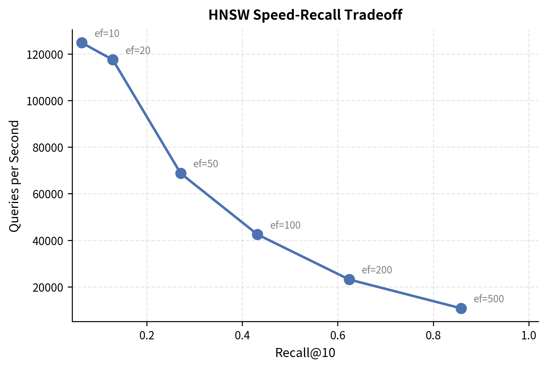
The beauty of HNSW is that ef_search can be tuned after building the index. We search with several values to observe the speed-recall tradeoff:
This table reveals the core tradeoff. Low ef_search values give blazing speed but miss some true nearest neighbors. As ef_search increases, recall climbs toward 1.0 (perfect), but each query takes longer. The sweet spot depends on your application: for RAG, a recall of 0.95 or higher is typically sufficient, since the reranker (which we'll cover in an upcoming chapter) can compensate for a few missed candidates.
Visualizing the Speed-Recall Tradeoff
Effect of M on Index Quality
We also examine how the connectivity parameter affects both memory and recall:
Higher values produce better recall because the denser graph provides more paths to reach any target. However, construction time also increases because each insertion requires evaluating more potential neighbors. For most practical applications, offers a good balance.
Memory Usage Analysis
Understanding HNSW's memory footprint is important for capacity planning. The index stores both the raw vectors and the graph structure:
The graph overhead is significant, roughly proportional to . For high-dimensional embeddings (d=768 or d=1536), the vectors dominate memory usage. But for lower-dimensional data, the graph structure can be a substantial fraction of total memory. This is one reason why techniques like Product Quantization, which we'll explore in an upcoming chapter, are often combined with HNSW to compress the stored vectors.
Using HNSW with FAISS
FAISS (Facebook AI Similarity Search) is another popular library that implements HNSW. Here's how the same index looks in FAISS:
The results demonstrate that FAISS achieves high recall with millisecond-latency search, comparable to the hnswlib implementation. FAISS's IndexHNSWFlat stores full (uncompressed) vectors. FAISS also supports combining HNSW with Product Quantization for compressed storage, which is especially useful when memory is constrained.
Key Parameters
The key parameters for HNSW are:
- M: Maximum number of connections per node. Controls graph density, memory usage, and recall.
- ef_construction: Size of the dynamic candidate list during index construction. Higher values improve index quality but slow down building.
- ef_search: Size of the dynamic candidate list during search. Higher values improve recall but increase latency.
Limitations and Impact
HNSW has become the de facto standard for approximate nearest neighbor search in production vector databases, and for good reason: it delivers consistently high recall with low latency across a wide range of data distributions and dimensionalities. However, no algorithm is without trade-offs, and understanding HNSW's limitations is crucial for making informed design decisions.
The most significant limitation is memory consumption. HNSW requires storing the entire graph structure in RAM, including all vectors and their neighbor lists. For a billion-vector index with 768-dimensional embeddings, the vectors alone require about 3 TB of storage (at 4 bytes per float), and the graph adds substantial overhead on top of that. This makes pure HNSW impractical for very large-scale deployments without compression techniques like Product Quantization or dimensionality reduction. In contrast, disk-based approaches like IVF indices (covered in the next chapter) can handle much larger collections because they only need to load a small subset of vectors into memory for each query.
Another limitation is the construction cost. Building an HNSW index is relatively slow compared to partition-based methods like IVF, because each insertion requires searching the existing graph to find neighbor candidates. The index also cannot be easily split across machines for distributed construction. Furthermore, HNSW indices are append-only in practice: while it's possible to add new vectors incrementally, deleting vectors is not natively supported in most implementations (deleted nodes leave "holes" in the graph that degrade connectivity over time). This makes HNSW less suitable for collections that change frequently, unless you periodically rebuild the index.
The tuning complexity is another practical concern. While HNSW has only three main parameters (, ef_construction, ef_search), finding the right settings for a given dataset and latency budget requires experimentation. The optimal parameters depend on the data dimensionality, distribution, and the required recall level, and these interactions are not always intuitive.
Despite these limitations, HNSW's impact on the field of vector search has been enormous. Before HNSW, you had to choose between tree-based methods (like KD-trees, which deteriorate badly in high dimensions), hash-based methods (like LSH, which require many hash tables for good recall), and simpler graph-based methods (which lacked the hierarchical navigation). HNSW provided a single algorithm that works well across the board, and its tunable speed-recall tradeoff made it practical for both latency-sensitive online serving and batch offline processing. Today, virtually every major vector database, including Pinecone, Weaviate, Qdrant, Milvus, and Chroma, uses HNSW as either its primary or default index type.
Summary
HNSW (Hierarchical Navigable Small World) is a graph-based approximate nearest neighbor algorithm that enables fast vector search by combining two key ideas:
-
Navigable Small World graphs provide a structure where greedy routing efficiently finds nearby nodes using only local information. Dense local connections enable precise search, while long-range connections enable fast traversal across the space.
-
Hierarchical layering (inspired by skip lists) separates coarse navigation from fine-grained search. Upper layers contain sparse subsets of nodes with naturally long-range connections. The bottom layer contains all nodes with dense short-range connections.
The algorithm's behavior is controlled by three parameters:
- : Connections per node (typically 16). Controls the density of the graph, affecting recall, memory, and speed.
ef_construction: Beam width during index building (typically 100-200). Higher values produce a better graph at the cost of slower construction.ef_search: Beam width during search (tunable at query time). Directly controls the speed-recall tradeoff.
Search works in two phases: greedy descent through upper layers (fast, coarse navigation), then beam search on layer 0 (thorough, precise retrieval). This structure achieves search complexity, making it practical for millions or billions of vectors.
HNSW's main limitations are its memory requirements (full graph must fit in RAM) and the difficulty of handling deletions. For collections too large to fit in memory, partition-based indices like IVF (covered in the next chapter) and compression techniques like Product Quantization offer complementary solutions. In practice, many production systems combine these approaches, using HNSW as the search graph within each partition of a larger index.
Quiz
Ready to test your understanding? Take this quick quiz to reinforce what you've learned about HNSW Index.

Comments