

Explore vector similarity search for RAG systems. Compare cosine, dot product, and Euclidean metrics, and implement exact vs. approximate search with FAISS.

This article is part of the free-to-read Language AI Handbook
Choose your expertise level to adjust how many terms are explained. Beginners see more tooltips, experts see fewer to maintain reading flow. Hover over underlined terms for instant definitions.
execute: cache: true jupyter: python3
Vector Similarity Search
In the previous chapter, we explored how embedding models transform text into dense vectors that capture semantic meaning. In the chapter on dense retrieval, we saw how these embeddings power modern search by finding documents whose vectors are "close" to a query vector. However, we need to define what "close" means and how to find the closest vectors efficiently in large collections.
This is the problem of vector similarity search. At small scales, it is trivially solved: compare the query to every vector in your collection and return the best matches. For large-scale RAG systems, this brute-force approach is often too slow. A collection of 10 million documents with 768-dimensional embeddings requires roughly 7.7 billion floating-point operations per query, just for a single distance metric. Handling thousands of concurrent users requires a more efficient approach.
This chapter lays the groundwork for efficient vector search. We start by examining the distance metrics that define what similarity means in vector space. Then we contrast exact search (which guarantees finding the true nearest neighbors) with approximate search (which trades a small amount of accuracy for dramatic speed improvements). Finally, we survey the libraries that implement these ideas and walk through practical code for each approach. The specific index structures that make approximate search possible, including HNSW and IVF, are covered in dedicated chapters that follow.
Distance Metrics
Before you can search for the "most similar" vectors, you need to define a measure of similarity. This decision shapes the entire retrieval pipeline. The metric you choose determines which documents appear at the top of your search results, how your index structures organize the vector space, and ultimately how effective your retrieval pipeline will be. Different metrics capture different geometric relationships between vectors, and understanding these relationships in detail is essential for building high-quality search systems.
At a high level, the question of similarity can be split into two perspectives. One perspective asks: "Are these two vectors pointing in roughly the same direction?" This is a question about orientation, about the angle between the arrows in vector space. The other perspective asks: "How far apart are these two vectors as points in space?" This is a question about position, about the absolute gap between them. These perspectives can yield different answers for the same pair of vectors. Knowing which question matters for your application helps in choosing the right metric.
Cosine Similarity
Cosine similarity measures the angle between two vectors, ignoring their magnitudes entirely. The core intuition is geometric: imagine two arrows emanating from the origin in a high-dimensional space. If the arrows point in the same direction, regardless of whether one is short and the other is long, we consider them maximally similar. If they point in perpendicular directions, they share no similarity at all. And if they point in opposite directions, they are maximally dissimilar. This is precisely what the cosine of the angle between two vectors captures.
For vectors and in , cosine similarity is defined as:
where:
- : the input vectors being compared
- : the dimensionality of the vector space
- : the scalar components of vectors and at dimension
- : the dot product, representing unnormalized alignment
- : the Euclidean length ( norm) of vector
- : the summation across all dimensions
To understand what this formula is really doing, let's break it apart. The numerator, the dot product , computes a raw measure of how well the two vectors align. It multiplies corresponding components and sums the results. When both vectors have large positive values in the same dimensions, the dot product grows large and positive. When one vector is positive where the other is negative, those dimensions contribute negative terms, pulling the sum down. The dot product, in isolation, reflects both alignment and magnitude: longer vectors produce larger dot products even at the same angle.
The denominator corrects for this magnitude dependence. By dividing by the product of the two vector norms, we effectively scale the dot product so that it reflects only the angular relationship. Geometrically, this is equivalent to first projecting both vectors onto the unit sphere (normalizing them to length 1) and then computing their dot product. The result is the cosine of the angle between them.
The result ranges from (pointing in opposite directions) through (orthogonal) to (pointing in the same direction). In practice, most embedding models produce vectors that occupy a relatively narrow region of the space, so similarity values for relevant documents often fall between 0.5 and 0.95.
Why is cosine similarity the default for text embeddings? Because it focuses on the direction of the vector rather than its length. Two documents about the same topic should be considered similar even if one has a larger-magnitude embedding. By normalizing out magnitude, cosine similarity captures pure semantic orientation. Consider two sentences like "The cat sat on the mat" and "A feline rested upon the rug." An embedding model should map these to vectors pointing in nearly the same direction, reflecting their shared meaning. Even if the model produces vectors of slightly different lengths for these two inputs, cosine similarity will correctly identify them as highly similar because their angular separation is small.
Search systems often need a distance (where smaller is better) rather than a similarity (where larger is better). Cosine distance is simply , converting the similarity into a value between 0 and 2 where 0 means identical direction.
Dot Product (Inner Product)
The dot product is the simplest and most computationally inexpensive of all vector similarity measures. It requires no normalization step: you simply multiply corresponding components and sum:
where:
- : the input vectors
- : the dimensionality of the vector space
- : the scalar components of vectors and at dimension
- : the summation across all dimensions
- : the aggregate alignment score, which increases with both directional similarity and vector length
Unlike cosine similarity, the dot product does account for vector magnitude. This means a longer vector can score higher even if its direction is slightly less aligned. To see why, think of it geometrically: the dot product of two vectors equals . When the norms are not divided out, a vector that is twice as long contributes twice as much to the final score, all else being equal. This makes the dot product sensitive to both how well two vectors agree in direction and how "strong" or "confident" each vector's representation is.
When would you want this behavior? When magnitude carries information. Some embedding models and retrieval systems train embeddings so that the vector norm encodes confidence or relevance strength. For example, a model might learn to produce longer vectors for documents that are more central to a topic and shorter vectors for documents that touch on the topic only tangentially. In these cases, dot product is the correct metric because it rewards both directional alignment and strong confidence signals. A highly relevant document with a long vector and good directional alignment will outscore a marginally relevant document, even if the marginal document happens to have a slightly better angle.
There is an important relationship between these two metrics that has profound practical consequences. If your vectors are -normalized (i.e., ), then the dot product and cosine similarity are identical:
where:
- : the normalized input vectors
- : the lengths of the vectors (both equal to 1)
- : the angle between vectors and
The derivation proceeds by recalling that the geometric definition of the dot product relates it to the product of the vector magnitudes and the cosine of the angle between them. When both vectors lie on the unit sphere, their magnitudes are exactly 1, and the product collapses to the cosine of the angle alone.
This is why many systems pre-normalize their embeddings. It lets you use the cheaper dot product operation while getting cosine similarity results, and it opens the door to optimized index structures that assume unit-norm vectors. The dot product avoids the division and square root operations required by cosine similarity, making it faster in tight inner loops where billions of comparisons are performed. By paying the one-time cost of normalization at indexing time, you gain this computational advantage at every subsequent query.
Euclidean Distance
Euclidean distance ( distance) takes an entirely different perspective from the angle-based metrics we have discussed so far. Instead of asking how well two vectors align directionally, it asks: how far apart are these two points in space? It measures the straight-line distance between two points, the length of the shortest path connecting them:
where:
- : the input vectors
- : the dimensionality of the vector space
- : the scalar components of vectors and at dimension
- : the difference between the scalar components along dimension
- : the squared difference, which makes negative differences positive and penalizes large outliers
- : the sum of squared differences across all dimensions
- : the square root, which converts the sum of squares back to the original units (linear distance)
This is the most intuitive metric: it corresponds to the physical distance you would measure with a ruler. It generalizes the familiar Pythagorean theorem from two or three dimensions to arbitrarily high-dimensional spaces. In two dimensions, the distance between points and is . The formula above extends this same idea to dimensions, summing the squared differences along every axis and taking the square root of the total.
Euclidean distance is sensitive to both direction and magnitude. Two vectors can have high cosine similarity (similar direction) but large Euclidean distance (very different magnitudes). Consider a query vector and a document vector . Their cosine similarity is a perfect 1.0, since they point in exactly the same direction. But their Euclidean distance is , which could be quite large. This illustrates the fundamental distinction: cosine similarity sees these as identical, while Euclidean distance sees them as far apart. Which perspective is "correct" depends entirely on whether magnitude carries meaningful information in your embedding space.
Another important property of Euclidean distance is its sensitivity to outlier dimensions. Because differences are squared before summing, a single dimension with a large discrepancy can dominate the total distance. For example, if two 768-dimensional vectors agree perfectly in 767 dimensions but differ by 10 in the remaining dimension, the squared Euclidean distance is , equivalent to disagreeing by 0.36 across all 768 dimensions. This squaring effect means Euclidean distance penalizes concentrated disagreement more heavily than diffuse disagreement.
For normalized vectors, Euclidean distance and cosine similarity are monotonically related. This connection is one of the most important results in vector similarity search, because it means that, under normalization, the choice between these two metrics does not change the ranking of results. The derivation proceeds by expanding the squared Euclidean distance:
where:
- : the squared Euclidean distance
- : the normalized input vectors (length of 1)
- : the angle between vectors and
The key step is the expansion in the second line. When you compute , you are effectively computing , which is . For unit vectors, the squared norms are both 1, and the dot product is , giving us the clean relationship .
So . Higher cosine similarity means smaller Euclidean distance. This means that for normalized vectors, searching by minimum Euclidean distance produces the same ranking as searching by maximum cosine similarity. The two metrics induce identical orderings over all candidate vectors, differing only in the numerical values they assign. In practice, many libraries use squared Euclidean distance () to avoid the square root computation, since it preserves the same ordering. The square root is a monotonically increasing function, so removing it does not affect which vector is closest or the relative ranking of candidates.
Manhattan Distance
Manhattan distance ( distance) takes yet another approach to measuring separation between points, one that treats each dimension independently and sums their contributions linearly rather than quadratically:
where:
- : the input vectors
- : the dimensionality of the vector space
- : the scalar components of vectors and at dimension
- : the absolute difference along dimension
- : the sum of these linear differences, representing the total "grid-based" distance
Named after the grid-like street layout of Manhattan, where travel between two points must follow the rectangular street grid rather than cutting diagonally, this metric captures a different notion of separation. Imagine navigating from one intersection to another: you can only move north-south or east-west, never diagonally. The total distance you travel is the sum of horizontal and vertical displacements, which is exactly what the norm computes.
This metric is less common for dense text embeddings but appears in some specialized contexts. It is more robust to outliers in individual dimensions than Euclidean distance, since it does not square the differences. Recall that in Euclidean distance, a single dimension with a discrepancy of 10 contributes 100 to the sum, whereas in Manhattan distance, it contributes only 10. This means Manhattan distance treats every unit of disagreement equally, regardless of whether it is concentrated in one dimension or spread across many. For representations where individual dimensions can occasionally take on extreme values, such as certain sparse or quantized embeddings, this robustness can be advantageous.
Choosing the Right Metric
The "correct" metric depends on how your embeddings were trained. This is a point worth emphasizing: the metric is not a free parameter you can tune independently. During training, the embedding model learns to arrange vectors in space so that a specific notion of similarity (defined by the training loss) corresponds to semantic relatedness. If the model was trained to make relevant document-query pairs have high cosine similarity, then the learned geometry of the embedding space is shaped around angular relationships. Using a different metric at search time than the one used during training will degrade retrieval quality, because you would be measuring a geometric property that the model did not optimize for.
Most modern sentence embedding models, including those we discussed in the previous chapter on embedding models, are trained with cosine similarity as the objective and expect you to use cosine similarity (or equivalently, dot product on normalized vectors) at search time.
The key guidelines are:
- Cosine similarity / normalized dot product: Default choice for most sentence embedding models (Sentence-BERT, E5, GTE, etc.)
- Dot product: Use when your model explicitly trains with dot product and encodes meaningful information in vector magnitude
- Euclidean distance: Common in computer vision embeddings and some specialized models; equivalent to cosine for normalized vectors
- Manhattan distance: Rarely the best choice for text embeddings, but useful for certain sparse or quantized representations
Exact Search: The Brute-Force Baseline
The simplest approach to finding the nearest neighbors of a query vector is exhaustive search: compute the distance between the query and every vector in the collection, then return the closest ones. Despite its simplicity, this approach serves a crucial role in the vector search ecosystem. It provides a correctness baseline against which all approximate methods are measured, and it remains the practical choice for collections small enough that its linear cost is acceptable.
How It Works
Given a query vector and a collection of vectors , each also in , exact search performs the following:
- Compute for all
- Sort or partially sort the results to find the smallest distances
- Return the corresponding vectors (and their identifiers)
The first step is where nearly all the computation happens. For each of the vectors in the collection, we must compute a distance or similarity score against the query. Each such computation involves multiplications and additions (for the dot product), plus any additional operations required by the specific metric (normalization for cosine similarity, subtraction and squaring for Euclidean distance). The computational cost is therefore for the distance computations, plus for maintaining a heap of the top results. For typical embedding dimensions ( to ) and collection sizes ( in the millions), the term dominates.
The second step, finding the top results, is handled efficiently by maintaining a max-heap (for distances, where we want the smallest) or min-heap (for similarities, where we want the largest) of size . As each new distance is computed, it is compared against the worst element in the heap. If the new distance is better, it replaces the worst element. This avoids the cost of fully sorting all distances and instead requires only operations, which is significantly cheaper when is small relative to .
Why It Matters
Exact search guarantees returning the true nearest neighbors. There are no missed relevant documents, no tuning parameters for recall, and no possibility that the correct answer was overlooked. Every vector in the collection is examined, so the algorithm has complete knowledge of the entire search space. This makes it the gold standard for evaluating approximate methods: when we report recall@k for an ANN algorithm, we are measuring how often it agrees with the results that exact search would have returned.
However, it scales linearly with collection size, making it inefficient for large datasets. Let's think through the numbers to develop a concrete sense of where the boundary lies. If you have 1 million vectors of dimension 768, a single query requires roughly 768 million multiply-add operations. On modern hardware with SIMD instructions, you can sustain around 10-50 billion floating-point operations per second on a single CPU core. That puts brute-force at roughly 15-75 milliseconds per query, which is potentially acceptable for some applications. But scale to 100 million vectors and you are looking at 1.5-7.5 seconds per query, which is far too slow for interactive use. The linear scaling with collection size means that every 10x increase in collection size produces a 10x increase in query time, with no way to mitigate this, short of faster hardware.
The story changes somewhat if you have GPUs available. Matrix-vector multiplication is massively parallel, and batching multiple queries together turns the problem into a matrix-matrix multiplication that modern GPUs handle extremely efficiently. Libraries like FAISS exploit this to make exact search surprisingly fast on GPU, even at moderate scales.
Space Complexity
Exact search requires storing all vectors in memory, since any vector could potentially be a nearest neighbor and must be accessible for the distance computation. For vectors of dimension stored as 32-bit floats, the memory requirement is:
where:
- : the number of vectors in the collection
- : the dimensionality of each vector
- : the size in bytes of a standard 32-bit floating-point number
This formula reflects the fact that each vector is simply a flat array of floating-point values, and the full collection is such arrays stored contiguously. There is no overhead for index structures in exact search: the "index" is just the raw matrix of vectors.
For 10 million vectors at dimension 768, that is about 28.8 GB. This is feasible on a single machine but becomes challenging at larger scales. We will see in the chapter on Product Quantization how vector compression can dramatically reduce this memory footprint.
Approximate Nearest Neighbor Search
The key insight behind approximate nearest neighbor (ANN) search is that you rarely need the exact nearest neighbors. In most retrieval applications, the downstream task (such as generating an answer from retrieved documents) is robust to small perturbations in the retrieved set. If the true 3rd-closest document has a similarity of 0.873 and the ANN algorithm returns a document with similarity 0.871 instead, the difference is negligible for downstream generation. The answer produced by the language model will be virtually indistinguishable regardless of which document was included.
By accepting this small accuracy trade-off, ANN algorithms can reduce search time from linear in to sublinear, often logarithmic or even near-constant. This is a dramatic improvement. Whereas exact search over 100 million vectors might take several seconds, a well-tuned ANN index can return results in a few milliseconds, a speedup of three orders of magnitude. This is what makes real-time retrieval over massive collections feasible.
A family of algorithms that find vectors approximately close to a query vector, trading a controlled amount of accuracy for dramatically faster search. The accuracy trade-off is typically measured by recall@k, the fraction of the true nearest neighbors that the approximate method successfully returns.
The Speed-Accuracy Trade-off
Every ANN algorithm offers knobs that control this trade-off. Turning the knob toward more accuracy means searching more of the index, examining more candidates, and spending more time verifying potential neighbors. Turning it toward more speed means searching less of the index, examining fewer candidates, and accepting a higher risk of missing relevant results. The art of ANN tuning is finding the sweet spot where recall is high enough (typically 95-99%) while latency meets your application requirements.
This trade-off is not binary: it is a continuous spectrum. For a given index structure, you can choose any operating point along a curve that runs from very fast and low recall to slow and perfect recall. This trade-off is usually visualized as a recall-vs-queries-per-second curve. A well-designed index will have an "elbow" where you get most of the recall for a modest time investment, with diminishing returns beyond that point. The ideal operating point is typically just past this elbow, where you have captured the vast majority of relevant neighbors while keeping latency well within your budget.
Families of ANN Approaches
ANN algorithms generally fall into several broad categories, each based on a different strategy for avoiding the exhaustive scan over all vectors. Understanding these families at a conceptual level helps you reason about which approach is best suited to your scale, hardware, and accuracy requirements:
- Tree-based methods: Partition the vector space using trees (e.g., KD-trees, random projection trees). Fast for low-dimensional data but struggle in high dimensions due to the curse of dimensionality.
- Hash-based methods: Use locality-sensitive hashing (LSH) to map nearby vectors to the same hash bucket. Simple and parallelizable, but often require many hash tables for good recall.
- Graph-based methods: Build a proximity graph where each vector is connected to its neighbors, then search by traversing the graph from a starting point toward the query. This family includes HNSW (Hierarchical Navigable Small World graphs), which is currently the most popular ANN method and the subject of the next chapter.
- Quantization-based methods: Compress vectors into compact codes, then search in the compressed space. Product Quantization (PQ) is the most well-known technique and is covered in a dedicated chapter ahead.
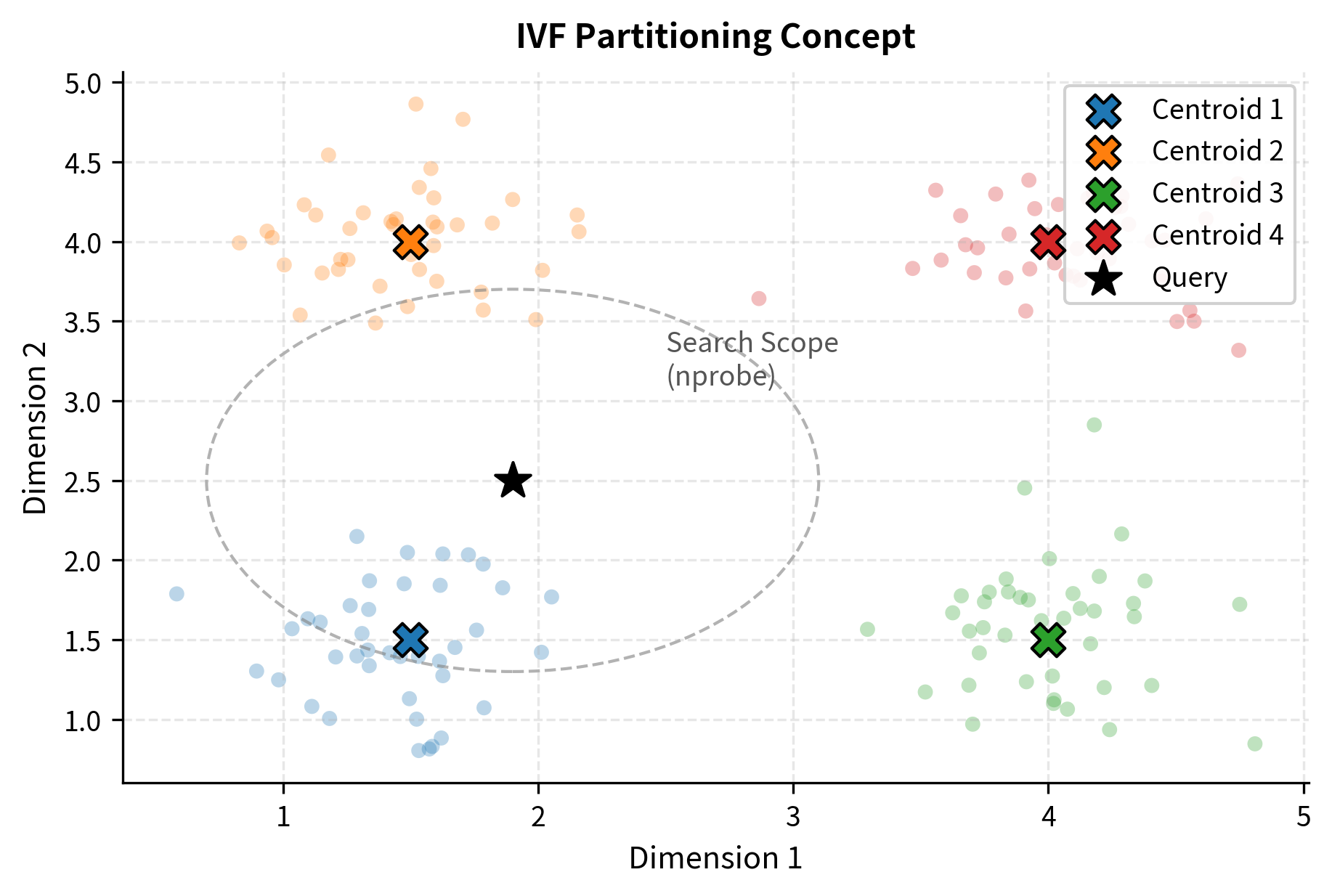
- Inverted file methods: Partition vectors into clusters (using k-means or similar), then search only the clusters closest to the query. The IVF index is one of the most widely used implementations and is also covered in an upcoming chapter.
In practice, production systems often combine multiple approaches. For example, FAISS's IVF_PQ index uses inverted file partitioning with product quantization for the vectors within each partition. Understanding the individual building blocks is essential for understanding these combinations.
Measuring ANN Quality
To compare ANN algorithms and tune their parameters, we need a principled way to measure how close an approximate result is to the true answer. The standard metric for ANN quality is recall@k, which directly measures the overlap between the approximate results and the exact results:
where:
- : the set of document identifiers returned by the approximate search
- : the set of document identifiers returned by an exact (brute-force) search
- : the cardinality (count) of the intersection between the two sets
- : the number of neighbors requested
The numerator counts how many of the true nearest neighbors actually appear in the ANN result set. The denominator normalizes by , the total number of neighbors requested, so that the metric always falls between 0 and 1. A recall of 1.0 means the ANN algorithm returned exactly the same set of neighbors as exact search (though possibly in a different order). A recall of 0.0 means it missed every single true neighbor.
To make this concrete with an example: if the true 10 nearest neighbors are documents {A, B, C, D, E, F, G, H, I, J} and your ANN algorithm returns {A, B, C, D, E, F, G, H, K, L}, then . The algorithm found 8 of the 10 true nearest neighbors, missing I and J while incorrectly including K and L. Note that the documents K and L are not necessarily irrelevant; they are simply not among the true top 10. In most practical scenarios, the documents that ANN returns instead of the missed true neighbors tend to have very similar scores, since the "mistakes" typically involve swapping neighbors that are nearly equidistant from the query.
For RAG applications, values above 0.95 are typically sufficient. The reranking stage that follows retrieval (which we will cover later in this part) can further compensate for occasional misses.
Worked Example: Metrics in Action
Let's make these metrics concrete with a small example that illustrates the key differences between direction-based and position-based measures. Suppose we have a query vector and four document vectors, all in for visualization simplicity. The low dimensionality lets us reason about the geometry directly, and the principles we observe generalize straightforwardly to the hundreds of dimensions used in real embeddings.
These four vectors were chosen deliberately to illustrate specific geometric relationships. Notice that , so it points in exactly the same direction but has 3 times the magnitude. This makes it a perfect test case for the distinction between direction-based and position-based metrics: any direction-based metric will consider identical to , while any position-based metric will see them as far apart. Meanwhile, , pointing in the exact opposite direction, which should produce the worst possible cosine similarity. The vector is the subtlest case: it is close to in both direction and magnitude, differing only by small perturbations in each component. Finally, points in a substantially different direction, with a large component in the third dimension where has only a small value.
Cosine similarity between and should be 1.0 (identical direction), while cosine similarity between and should be (opposite direction). Meanwhile, is close to in both direction and magnitude, so it should also have high cosine similarity, though not a perfect 1.0.
Euclidean distance between and should be small (they are nearby), while the distance between and will be large despite their identical directions (because is far away in absolute terms). This is the signature behavior that distinguishes position-based from direction-based metrics.
This example highlights the core difference between direction-based metrics (cosine) and position-based metrics (Euclidean): whether magnitude matters or not.
The results confirm our predictions. By cosine similarity, scores a perfect 1.0 (same direction as the query) while scores (opposite direction). But by Euclidean distance, is the closest neighbor (only 0.1732 away), while is much farther despite its perfect directional alignment.
This illustrates why the choice of metric matters. If you rank by cosine similarity, is the top result. If you rank by Euclidean distance, wins. Neither answer is "wrong"; they are answering different questions about what "similar" means. Cosine similarity asks, "Which document is most topically aligned with the query?" Euclidean distance asks, "Which document is closest to the query in the embedding space?" For normalized vectors these questions have the same answer, but for unnormalized vectors they can diverge significantly, as this example demonstrates.
Now let's see what happens when we normalize the vectors:
After normalization, cosine similarity and dot product produce identical values, confirming the mathematical relationship we derived earlier: for unit vectors, . And the rankings from all three metrics now agree: the vectors with higher cosine similarity also have smaller Euclidean distance, exactly as the identity predicts. Notice in particular that , which was far from the query before normalization, now sits at exactly the same point as the normalized query, with Euclidean distance 0.0. Normalization collapsed the magnitude information and left only direction.
This is the practical reason why normalizing embeddings before indexing is so common: it makes the choice of metric irrelevant. Once all vectors lie on the unit sphere, cosine similarity, dot product, and Euclidean distance all induce the same ranking over candidates. You can then choose whichever metric your library computes most efficiently, typically the dot product, without worrying about whether it matches the conceptual notion of similarity your model was trained with.
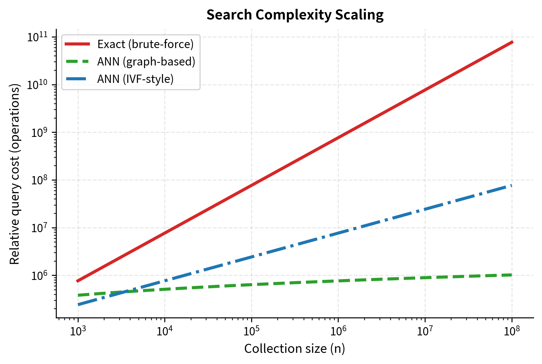
Complexity Comparison
Understanding the computational complexity of different search strategies helps you make informed decisions about which approach fits your scale. The differences between exact and approximate search are not marginal: they are qualitative changes in how query cost grows with collection size. Exact search grows linearly, meaning that doubling the collection size doubles the query time. Approximate methods grow sublinearly, meaning that doubling the collection size increases query time by much less than a factor of two. At large scales, this distinction is the difference between a system that responds in milliseconds and one that takes seconds.
The table below summarizes the trade-offs across the major search strategies. Each row captures a different aspect of system behavior, from query-time latency to memory consumption, and the columns reveal how these aspects vary across the four principal approaches. Reading across a row lets you compare one property across all strategies; reading down a column gives you the full profile of a single strategy.
| Property | Exact Search | Graph-based ANN | IVF-based ANN | Quantized ANN |
|---|---|---|---|---|
| Query time | , | |||
| Index build time | ||||
| Memory | ||||
| Recall guarantee | 100% | Tunable (95-99%+) | Tunable (90-99%+) | Tunable (85-95%+) |
| Best for | Small collections, ground truth | Large-scale, low latency | Very large scale | Memory-constrained |
where:
- : the number of graph connections per node (in HNSW)
- : the centroid storage cost (in IVF)
- : the number of clusters (in IVF)
- : the compressed dimension (in quantization methods)
- : the number of vectors in the collection
- : the dimensionality of the vector space
Several patterns in this table deserve attention. First, notice that exact search has index build time, because there is no index to build: you simply store the raw vectors. All approximate methods require an upfront investment in index construction, whether that is building a graph (HNSW), clustering vectors into partitions (IVF), or learning codebooks (quantization). This build cost is amortized over all future queries, making it worthwhile when the collection will be queried many times.
Second, observe the memory column. Graph-based methods add connections per vector on top of the full vector storage, which increases memory usage but enables the fast navigable graph traversal that gives HNSW its speed advantage. IVF methods add a relatively modest centroid storage cost (proportional to the number of clusters, not the number of vectors). Quantization methods achieve the greatest memory savings by replacing the full -dimensional vector with a compressed code of dimension , where can be 8 to 32 times smaller than .
The graph-based approach (HNSW) typically offers the best recall at a given query speed, which is why it has become the dominant ANN method. However, it uses more memory than quantization-based approaches because it stores both the full vectors and the graph edges.
Code Implementation with FAISS
FAISS (Facebook AI Similarity Search) is the most widely used library for vector similarity search. Developed by Meta AI, it provides efficient implementations of exact search, IVF, HNSW, PQ, and their combinations, with both CPU and GPU backends. Let's use it to compare exact and approximate search on a realistic dataset.
Setting Up and Generating Data
We will create a synthetic dataset that mimics the scale and dimensionality of a real embedding collection.
Our collection occupies about 146 MB, which is modest enough for exact search on a laptop. At 10x or 100x this scale, approximate methods become necessary.
Exact Search with FAISS
FAISS provides IndexFlatIP for exact inner product search and IndexFlatL2 for exact Euclidean distance search. Since our vectors are normalized, inner product is equivalent to cosine similarity.
The exact search returns the true nearest neighbors with cosine similarities. These results serve as our ground truth for evaluating approximate methods.
Approximate Search with IVF
The IVF (Inverted File) index partitions vectors into clusters, then only searches the clusters closest to the query. The nprobe parameter controls how many clusters to search: higher nprobe means higher recall but slower search.
You can see the speed-accuracy trade-off in action. With nprobe=1 (searching only the single nearest cluster), the search is very fast but misses some true neighbors. As nprobe increases, recall improves but search time grows. At nprobe=50 (searching half of all clusters), recall is typically near perfect, but the search is slower.
Approximate Search with HNSW
FAISS also provides an HNSW index, which builds a navigable graph structure. The key parameter is efSearch, which controls how many candidates to evaluate during the graph traversal.
HNSW generally achieves higher recall at lower latency than IVF for a given collection size. The next chapter dives deep into exactly how the HNSW graph structure achieves this.
Visualizing the Trade-off
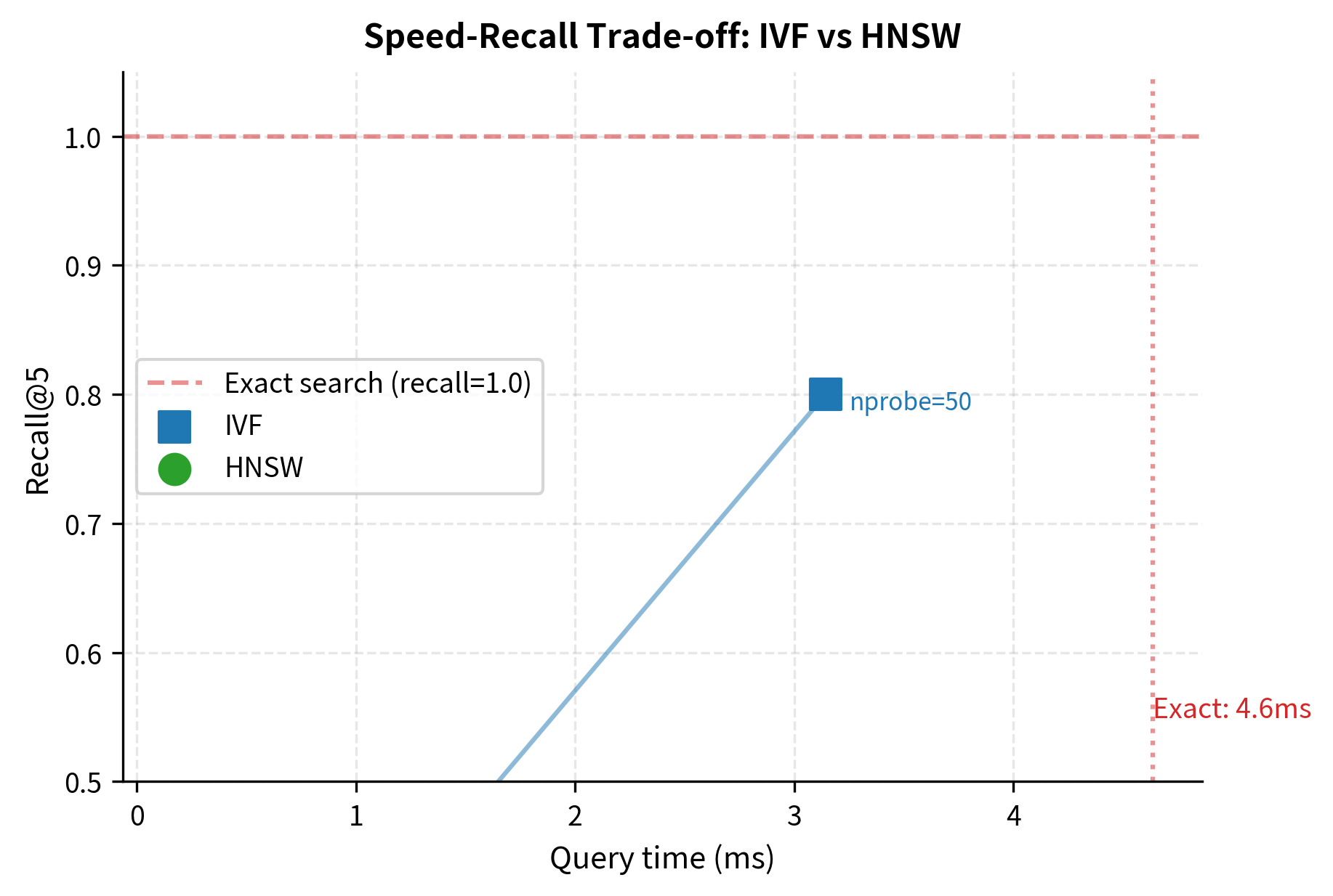
The plot shows the fundamental trade-off that defines ANN search. Each point represents a different parameter setting, and the goal is to get as close to the upper-left corner as possible (high recall, low latency). In practice, you would benchmark your specific collection and choose the operating point that balances your latency budget with your recall requirements.
Key Parameters
The key parameters for the FAISS index implementations are:
- n_clusters: The number of clusters (Voronoi cells) to partition the vector space into for the IVF index.
- nprobe: The number of closest clusters to search during an IVF query. Higher values increase recall but reduce speed.
- M: The number of edges (neighbors) per node in the HNSW graph. Controls the graph connectivity and memory usage.
- efSearch: The size of the dynamic candidate list during HNSW search. Higher values improve recall at the cost of latency.
Similarity Search Libraries
FAISS is the most established library, but the vector search ecosystem has grown rapidly. Here is a brief overview of the major options:
-
FAISS (Meta): The gold standard for research and production. Supports CPU and GPU, with extensive index types (Flat, IVF, HNSW, PQ, and combinations). Written in C++ with Python bindings. Best for you if you need fine-grained control over index construction.
-
Annoy (Spotify): Uses random projection trees. Simple API, memory-maps indexes for efficient loading, and supports sharing indexes across processes. Good for medium-scale applications where simplicity matters. Does not support adding vectors after index construction.
-
ScaNN (Google): Optimized for inner product search with a technique called anisotropic vector quantization. Achieves state-of-the-art speed-recall trade-offs on several benchmarks. Good for production systems that need the best possible performance.
-
HNSWlib: A standalone C++ implementation of the HNSW algorithm with Python bindings. Lighter weight than FAISS, focused exclusively on the HNSW index type. A good choice if you only need HNSW and want minimal dependencies.
-
Qdrant, Milvus, Weaviate, Pinecone: These are full vector databases rather than libraries. They add persistence, filtering, distributed search, and managed hosting on top of the core ANN algorithms. We will discuss the distinction between vector search libraries and vector databases when we cover RAG system architecture.
For this chapter, we have focused on FAISS because of its versatility and widespread adoption. The specific index structures it offers (HNSW, IVF, PQ) are explored in depth in the following chapters.
Limitations and Practical Considerations
Vector similarity search is powerful but comes with important caveats that affect real-world RAG systems.
A key limitation is that vector similarity is not semantic equivalence, as two documents can have high cosine similarity without being truly relevant to the query, and genuinely relevant documents can sometimes have lower similarity scores than irrelevant ones. This happens because embedding models compress complex, nuanced meaning into fixed-size vectors, and information is inevitably lost in this compression. A query about "python programming" might retrieve documents about actual pythons if the embedding model does not sufficiently distinguish context. This is one reason why RAG pipelines typically include a reranking stage (covered later in this part), which uses a more expensive cross-encoder model to rescore the top candidates.
The curse of dimensionality also affects ANN algorithms in subtle ways. In very high-dimensional spaces, the ratio between the nearest and farthest neighbor distances shrinks, making all vectors appear roughly equidistant. Typical embedding dimensions (384-1536) are high enough that this effect is noticeable but not catastrophic. However, it means that ANN algorithms cannot offer the same theoretical guarantees in high dimensions that they can in low dimensions. In practice, the learned structure of real embeddings (which are not uniformly distributed but cluster meaningfully) counteracts this effect, and ANN methods work much better on real data than worst-case theory would suggest.
Memory remains a persistent practical concern. Storing 100 million 768-dimensional vectors in float32 requires about 288 GB of RAM, before accounting for the additional memory needed by the index structure itself (graph edges for HNSW, centroid tables for IVF, etc.). Product Quantization and other compression techniques, which we cover in a dedicated chapter, can reduce this by 10-30x, but at the cost of reduced recall. Designing a system that balances memory, speed, and accuracy for a given hardware budget is one of the core engineering challenges in production RAG.
Finally, vector search indexes are generally static or semi-static. While some structures (like HNSW) support incremental insertion, most achieve their best performance when built once on the full dataset. Frequent updates, such as adding or deleting documents in real time, can degrade index quality or require expensive rebuilds. This matters for applications where the document collection changes continuously, and various strategies exist to handle it, from periodic index rebuilds to tiered architectures that combine a large static index with a small dynamic one.
Summary
This chapter established the foundations of vector similarity search, the core retrieval operation in any RAG pipeline.
Distance metrics define what "similar" means in vector space. Cosine similarity (direction-based) is the default for text embeddings, while dot product is equivalent for normalized vectors and Euclidean distance captures position-based proximity. Always match your search metric to your embedding model's training objective.
Exact search computes distances against every vector in the collection, guaranteeing perfect recall at cost per query. It is practical for small collections (under ~1 million vectors) but does not scale.
Approximate Nearest Neighbor (ANN) algorithms achieve sublinear query time by sacrificing a small, controllable amount of recall. The key families are graph-based (HNSW), partition-based (IVF), and compression-based (Product Quantization), each offering different speed-memory-recall trade-offs tunable via parameters like efSearch and nprobe.
FAISS is the most widely used similarity search library, providing implementations of all major index types with both CPU and GPU backends. The recall-vs-speed trade-off curves we generated demonstrate how parameter tuning lets you find the right operating point for your application.
With the conceptual framework and metrics in place, the next three chapters dive into the specific index structures that make large-scale ANN search possible: HNSW graphs, IVF partitioning, and Product Quantization.
Quiz
Ready to test your understanding? Take this quick quiz to reinforce what you've learned about vector similarity search.

Comments