

Learn how embedding models convert text to vectors for RAG. Covers bi-encoder architecture, pooling strategies, dimensionality trade-offs, and model selection.

This article is part of the free-to-read Language AI Handbook
Choose your expertise level to adjust how many terms are explained. Beginners see more tooltips, experts see fewer to maintain reading flow. Hover over underlined terms for instant definitions.
Embedding Models
In the previous chapters on dense retrieval and contrastive learning, we established why we need dense vector representation, similar and how models learn to place semantically similar texts near each other. However, we did not address a critical question: how does a transformer, which produces a sequence of token-level hidden states, yield a single vector that represents an entire sentence or paragraph? The answer lies in the architecture and design choices of embedding models, the specialized systems that convert variable-length text into fixed-dimensional vectors suitable for similarity search.
Embedding models sit at the heart of every RAG pipeline. The quality of your retrieval, and therefore the quality of your generated answers, depends directly on how well your embedding model captures semantic meaning. A poorly chosen or misconfigured embedding model will return irrelevant chunks no matter how sophisticated the rest of your pipeline is.
This chapter examines embedding models from the inside out. We'll start with the architectural foundations, then explore the pooling strategies that collapse token representations into a single vector, discuss the role of embedding dimensionality, and conclude with practical guidance on selecting the right model for your use case.
From Token Embeddings to Sentence Embeddings
As covered in previous chapters, encoder models like BERT produce contextual token embeddings: one vector per input token, where each vector is influenced by the surrounding context through self-attention. A sentence of 12 tokens passed through BERT yields 12 vectors of dimension 768. But for retrieval, we need one vector per document chunk. The bridge between token-level representations and a single sentence-level vector is what defines an embedding model.
To appreciate why this bridge is non-trivial, consider the nature of the problem. A transformer encoder processes text through multiple layers of self-attention and feed-forward transformations, producing at each layer a set of contextualized representations, one per token. By the final layer, each token's hidden state is richly informed by all the other tokens in the input. Yet these representations remain anchored to individual token positions. There is no built-in mechanism in a standard transformer encoder that automatically distills an entire sequence's meaning into a single, compact vector. That distillation is precisely what an embedding model must accomplish, and the method it uses to do so has a significant impact on retrieval quality.
An embedding model is a neural network, typically built on a transformer encoder, that maps variable-length text to a fixed-dimensional vector. Unlike general-purpose language models, embedding models are specifically trained so that the geometric relationships between output vectors reflect semantic relationships between input texts.
The naive approach of simply using a pre-trained BERT model to generate sentence embeddings performs surprisingly poorly. Reimers and Gurevych (2019) demonstrated that averaging BERT's token embeddings without further training produces representations that are often worse than GloVe averages for semantic similarity tasks. The problem is that BERT's pre-training objectives (masked language modeling and next sentence prediction) optimize for token-level predictions, not for producing globally meaningful sentence vectors. In other words, BERT learns to predict missing words and to decide whether two sentences follow each other, but neither of these tasks requires the model to compress the holistic meaning of a sentence into a single point in vector space. The token-level hidden states carry abundant contextual information, but that information is distributed across positions in a way that does not naturally aggregate into a coherent whole without explicit guidance.
This insight motivated the development of dedicated embedding models: transformer encoders that are fine-tuned with objectives that explicitly shape the geometry of the output space. The contrastive learning techniques from the previous chapter are precisely how this fine-tuning is done. By training the model to push embeddings of semantically similar texts closer together while pulling embeddings of dissimilar texts apart, the fine-tuning process transforms a collection of token-level representations into a structured embedding space where distances carry genuine semantic meaning.
Embedding Model Architectures
Modern embedding models share a common blueprint, but they differ in their choice of base encoder, training procedure, and output processing. Understanding these architectural families helps clarify what happens under the hood when you call a model's encode method and receive a vector back. Let's examine the key architectural families, starting with the design that established the modern approach to sentence embeddings.
Sentence-BERT (SBERT) and the Bi-Encoder Pattern
Sentence-BERT, introduced by Reimers and Gurevych (2019), established the dominant paradigm for embedding models. The core idea is simple: take a pre-trained transformer encoder, add a pooling layer on top, and fine-tune the entire stack using siamese or triplet networks with a contrastive objective. What makes this approach so powerful is the combination of a strong pre-trained foundation, which provides rich contextual understanding of language, with a training objective that explicitly organizes the output space for semantic comparison.
The architecture uses what's called a bi-encoder (or dual-encoder) pattern, which we encountered in the dense retrieval chapter. The query and the document are encoded independently by the same model. This independence is what makes bi-encoders fast at retrieval time: document embeddings can be precomputed and indexed, and at query time only the query needs to be encoded. The key insight is that because the same encoder processes both queries and documents, both types of text are mapped into the same shared vector space. Proximity in this space reflects semantic similarity, regardless of whether the two texts being compared are both queries, both documents, or one of each.
The forward pass for a single input proceeds through four key steps:
- Tokenization: The input text is split into subword tokens using the encoder's vocabulary.
- Encoding: Tokens pass through the transformer layers, producing contextualized token embeddings.
- Pooling: A strategy like mean pooling reduces the token embeddings to a single vector.
- Normalization: Optionally, the vector is normalized (e.g., to unit length) or projected to a desired dimension.
Each of these steps involves design choices that affect the quality of the resulting embedding, and the pooling step in particular, which we will examine in depth shortly, is where much of the embedding model's character is determined.
Instructor and Task-Aware Models
A limitation of standard embedding models is that they produce the same vector for a piece of text regardless of the intended task. The text "Python is a programming language" gets the same embedding whether you're doing topic classification, semantic search, or clustering. This is a meaningful limitation because the aspects of a text that matter most depend entirely on how the embedding will be used. For a classification task, you might want the embedding to emphasize the category or topic of the text. For a semantic search task, you might want it to emphasize the specific facts or claims that a query could ask about. A single, task-agnostic embedding cannot optimally serve all of these purposes.
Task-aware models like Instructor (Su et al., 2023) address this by prepending a task instruction to each input. Instead of encoding just the text, you encode something like: "Represent the science document for retrieval: Python is a programming language." The instruction conditions the model to produce embeddings optimized for the specified task. By seeing the instruction as part of the input sequence, the model can learn to shift its internal representations, emphasizing different features depending on what the instruction asks for.
This approach doesn't require architectural changes; it leverages the transformer's ability to attend across the full input, including the instruction prefix. The model is trained on diverse tasks with diverse instructions, learning to shift its embedding space based on the instruction context. The result is a single model that behaves like many specialized models, adapting its output representations to the task at hand simply by reading a natural language instruction.
Late Interaction Models
While not strictly single-vector embedding models, late interaction architectures like ColBERT deserve mention because they represent a middle ground between bi-encoders and cross-encoders. The fundamental trade-off in retrieval model design is between expressiveness and efficiency. Bi-encoders are efficient because they compress each text to a single vector, but this compression sacrifices fine-grained token-level matching. Cross-encoders are expressive because they perform full token-level cross-attention between a query and a document, but this means the document cannot be pre-encoded independently of the query, making them too slow for first-stage retrieval over large corpora.
Late interaction models navigate this trade-off by retaining more information than bi-encoders while remaining far more efficient than cross-encoders. Instead of compressing each text into a single vector, ColBERT retains all token-level embeddings and computes similarity using a MaxSim operation: for each query token, find its maximum similarity to any document token, then sum these maximums. This mechanism allows ColBERT to capture fine-grained lexical and semantic matches between individual query terms and document terms, something that a single-vector comparison cannot achieve.
This preserves more fine-grained information than single-vector approaches while remaining more efficient than full cross-attention. We'll see how this fits into retrieval pipelines when we discuss reranking later in this part.
Modern Embedding Architectures
Recent embedding models have pushed performance significantly through several innovations. These advances reflect a broader trend in the field: rather than relying on a single breakthrough technique, the best embedding models combine multiple complementary strategies to achieve state-of-the-art results.
- Larger and better base models: Moving from BERT-base (110M parameters) to larger encoders or even decoder-based models. Models like E5-Mistral use a decoder-only LLM (Mistral 7B) as the backbone, applying special pooling to extract embeddings. The intuition here is that larger language models develop richer internal representations of language during pre-training, and these richer representations translate into more nuanced embeddings after fine-tuning.
- Multi-stage training: GTE, BGE, and E5 families use a progressive training pipeline: first pre-training on large weakly-supervised pairs (e.g., title-body pairs from the web), then fine-tuning on curated labeled data, and sometimes a final distillation stage. Each stage serves a distinct purpose: the first stage teaches the model about broad notions of textual relevance from massive data; the second stage refines this understanding using high-quality human judgments; and the optional distillation stage compresses knowledge from a larger teacher model into a smaller, faster student.
- Matryoshka representation learning: Training embeddings so that any prefix of the vector (the first 64, 128, or 256 dimensions) is itself a useful embedding, allowing flexible dimensionality at inference time. We will explore this technique in detail later in the chapter.
- Unified models for multiple tasks: Models like GTE-Qwen2 handle embedding, retrieval, reranking, and classification within a single architecture, using instructions to switch modes. This unification simplifies deployment because a single model can serve multiple roles in the pipeline.
Pooling Strategies
The pooling layer is arguably the most critical design choice in an embedding model. It determines how the rich, token-level information from the transformer is compressed into a single vector. To understand why this choice matters so much, consider what happens at the output of a transformer encoder. You have a matrix of hidden states, one row per token, each row a high-dimensional vector capturing that token's meaning in context. The pooling layer must somehow condense this entire matrix, which can have hundreds of rows, into a single row. Different strategies for performing this condensation emphasize different aspects of the input, and the choice of strategy interacts deeply with how the model was trained. Let's examine the main strategies, starting with the simplest.
CLS Token Pooling
BERT and its variants include a special [CLS] token at the beginning of every input. During pre-training, the hidden state corresponding to [CLS] is used as the "aggregate sequence representation" for the next sentence prediction task. CLS pooling simply takes this one vector as the sentence embedding. The idea is appealing in its simplicity: designate one specific position in the sequence as the "summary" position, and let the model learn to route all relevant information to that position through self-attention.
Formally, the CLS pooling operation extracts the hidden state at the very first position of the output:
where:
- : the resulting sentence embedding vector
- : the final hidden state vector corresponding to the special
[CLS]token
The appeal of CLS pooling is that the model has a dedicated token whose job is to aggregate information from the entire sequence. Through self-attention, the [CLS] token can attend to every other token, and the model can learn to pack a summary of the input into this position. Because self-attention allows every token to interact with every other token at each layer, the [CLS] token has, in principle, access to the full content of the input by the time it reaches the final layer. If the training objective rewards the [CLS] position for capturing the overall meaning of the input, the model has both the mechanism (self-attention) and the incentive (the loss function) to make this work.
However, CLS pooling has a significant weakness: the [CLS] token's representation is heavily shaped by its pre-training objective (next sentence prediction in BERT), which doesn't necessarily align with semantic similarity. The next sentence prediction task is a binary classification problem, asking whether sentence B follows sentence A in the original text. This is a coarse signal compared to the nuanced semantic distinctions required for retrieval, and it means the [CLS] representation may encode information useful for that binary decision but not for capturing the full semantic content of the input. Without fine-tuning specifically for embedding quality, [CLS] representations can be noisy and poorly calibrated. After proper contrastive fine-tuning, CLS pooling works well and is used by several strong models including the DeBERTa-based models and many decoder-based embedding models.
Mean Pooling
Mean pooling takes a fundamentally different approach from CLS pooling. Rather than relying on a single designated token to carry all the information, mean pooling distributes the responsibility across every token in the sequence. It computes the sentence embedding by averaging the hidden states of all input tokens, excluding padding tokens, to produce a single representative vector:
where:
- : the resulting sentence embedding vector
- : the set of indices corresponding to real (non-padding) tokens
- : the hidden state vector output by the transformer at position
- : the count of real tokens in the sequence
The intuition behind this formula is straightforward. Each token's hidden state, by the final layer of the transformer, encodes not just the meaning of that individual token but also its relationship to the surrounding context. By averaging all of these context-rich representations, mean pooling creates a vector that reflects the collective semantic content of the entire sequence. No single token is privileged, and the contributions of all tokens are weighted equally.
In practice, this is implemented using the attention mask to zero out padding positions before averaging. Padding tokens are added to make all sequences in a batch have the same length, but they carry no meaningful content and should not influence the embedding. The attention mask provides exactly the information needed to exclude them:
where:
- : the resulting sentence embedding vector
- : the total length of the tokenized sequence (including padding)
- : the attention mask value at position (1 for real tokens, 0 for padding)
- : the hidden state vector at position
The numerator sums only the hidden states of real tokens (since padding positions are multiplied by zero), while the denominator counts the number of real tokens (the sum of the mask values). This ensures that the average is taken only over meaningful positions, regardless of how much padding was added to the sequence.
Mean pooling is the most widely used strategy in modern embedding models, and for good reason. By averaging over all tokens, it captures information distributed across the entire sequence rather than relying on a single position. It's also more robust: no single token needs to carry all the information, so the model can distribute semantic content across positions naturally. This distribution is especially valuable for longer inputs, where important information may appear anywhere in the text, from the opening sentence to the final clause.
Sentence-BERT showed that mean pooling consistently outperforms CLS pooling when fine-tuning from a pre-trained BERT checkpoint. Most state-of-the-art models, including the E5, GTE, and BGE families, use mean pooling as their default strategy.
Weighted Mean Pooling
A refinement of mean pooling introduces position-dependent weights, allowing the model to emphasize certain token positions over others. Typically, later tokens in the sequence receive higher weight:
where:
- : the resulting sentence embedding vector
- : the total length of the tokenized sequence
- : the weight assigned to position (e.g., to prioritize later tokens)
- : the attention mask value (1 for real tokens, 0 for padding)
- : the hidden state vector at position
The intuition is that later layers' representations of later tokens have "seen" more context through causal or bidirectional attention, so they might carry more refined semantic information. In a bidirectional encoder, this intuition is less compelling because every token attends to every other token regardless of position. However, in models that use any form of positional bias, or in practice where certain positions tend to carry more salient information (such as the end of a sentence, which often contains the main predicate or conclusion), positional weighting can provide a small boost.
In practice, weighted mean pooling offers marginal improvements in some settings and is not widely adopted in production models. The added complexity of choosing a weighting scheme rarely justifies the modest gains, and standard mean pooling remains the preferred default.
Max Pooling
Max pooling takes the element-wise maximum across all token positions, selecting the strongest activation for each dimension independently:
where:
- : the value of the -th dimension in the final embedding vector
- : the set of non-padding token positions
- : the value of the -th dimension of the hidden state at token position
To understand what this formula does, consider a single dimension of the embedding. Across all the token positions in the input, each token's hidden state contributes a value for this dimension. Max pooling selects the largest of these values. The resulting embedding vector is assembled dimension by dimension, where each dimension's value comes from whichever token produced the strongest activation along that particular feature.
Max pooling captures the strongest activation for each feature dimension across the sequence. It can be effective when the presence of a particular feature (encoded in a dimension) anywhere in the text is more important than its average strength. For example, if a particular dimension activates strongly when the model detects a mention of a geographic location, max pooling will preserve that signal even if the location is mentioned only once in a long passage, whereas mean pooling would dilute it by averaging with all the other tokens where that dimension has lower activation. However, max pooling is sensitive to outlier activations and is rarely used as the sole pooling strategy in modern models, because a single anomalous token can dominate the embedding along many dimensions simultaneously.
Last Token Pooling
For decoder-only models like GPT or LLaMA that use causal attention, the information flow through the transformer has a distinct directional character. In causal attention, each token can attend only to itself and to tokens that precede it in the sequence. This means that the first token sees only itself, the second token sees the first and itself, and so on, with each successive token having access to a progressively larger window of context. The last token in the sequence is therefore the only position that has attended to all previous tokens, making it a natural candidate for pooling:
where:
- : the resulting sentence embedding vector
- : the hidden state vector at the last token position
This is the analog of CLS pooling for causal models, but the reasoning for using it is almost exactly reversed. In a bidirectional encoder, the [CLS] token at the beginning can attend to all other tokens through bidirectional self-attention, so it has access to the full input. In a causal decoder, it is the last token, not the first, that has this property. Since causal attention means earlier tokens cannot see later tokens, the first token (which CLS pooling would use) has the least context. The last token, having attended to the full prefix, carries the most information and serves as the most informed summary of the entire sequence.
Models like E5-Mistral and SFR-Embedding use this strategy. Some models append a special end-of-sequence token and use its representation, similar to how BERT uses [CLS] but at the end rather than the beginning. This special token acts as a dedicated aggregation point, giving the model a specific position where it can learn to concentrate the most important information about the input.
Comparing Pooling Strategies
The choice of pooling strategy interacts strongly with the model architecture and training procedure. This interaction is one of the most important things to understand about embedding models: a pooling strategy cannot be evaluated in isolation, because its effectiveness depends on how the model was designed and trained to use it. The following guidelines reflect best practices from the research literature:
- Encoder models (BERT, RoBERTa, DeBERTa): Mean pooling generally wins, though CLS pooling is competitive after proper fine-tuning. The bidirectional attention in these models means every token has access to the full input, so averaging across all positions captures a rich, balanced representation.
- Decoder-only models (Mistral, LLaMA, Qwen): Last token pooling is the natural choice due to causal attention masking. Only the final position has attended to the complete input, making it the only position with sufficient information to serve as a standalone summary.
- Encoder-decoder models (T5, BART): The encoder's output is typically mean-pooled, similar to encoder-only models. The encoder in these architectures uses bidirectional attention, so the same reasoning that favors mean pooling in encoder-only models applies here as well.
Let's implement the main pooling strategies and see how they differ in practice. We will encode three sentences, two semantically similar and one dissimilar, through the same model and apply each pooling method to the raw hidden states. By comparing the resulting cosine similarity matrices, we can observe how different pooling strategies affect the model's ability to distinguish related from unrelated texts.
We'll encode these sentences and extract the raw hidden states before applying different pooling strategies. By working with the raw outputs rather than the model's built-in encoding pipeline, we can apply each pooling strategy independently to the same set of hidden states, ensuring a fair comparison.
Now let's compare the cosine similarity matrices produced by each strategy. Cosine similarity measures the angle between two vectors, with values near 1.0 indicating that the vectors point in nearly the same direction (high semantic similarity) and values closer to 0 indicating that the vectors are nearly orthogonal (low semantic similarity). A good pooling strategy should produce high similarity between the two animal-on-surface sentences and lower similarity between either of those and the stock market sentence.
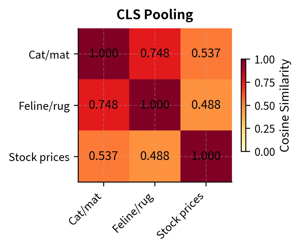
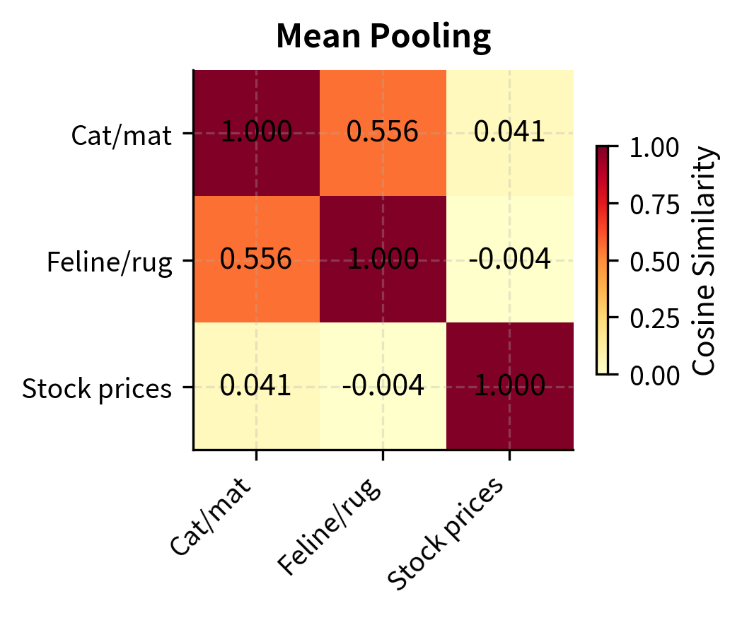
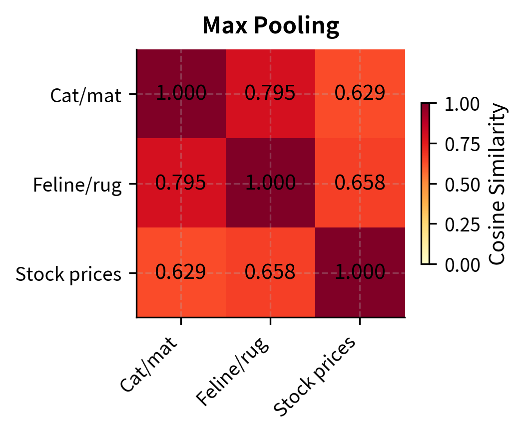
The heatmaps reveal the differences between pooling strategies. This particular model (all-MiniLM-L6-v2) was trained with mean pooling, so that strategy produces the most semantically meaningful similarities: the two animal-on-surface sentences are highly similar, while the stock market sentence is more distant. CLS and max pooling, applied to a model trained for mean pooling, produce less differentiated similarity scores. This underscores an important point: the pooling strategy must match what the model was trained with. Using CLS pooling on a model fine-tuned with mean pooling (or vice versa) will degrade quality.
Key Parameters
The key parameters for the tokenizer are:
- padding: Adds special padding tokens to ensure all sequences in a batch have the same length.
- truncation: Truncates sequences that exceed the model's maximum context length.
- return_tensors: Specifies the return type (e.g.,
"pt"for PyTorch) for compatibility with the model.
Embedding Dimensions
The dimensionality of the output embedding, the length of the vector, is a crucial parameter that affects retrieval quality, storage costs, and computation speed. Every embedding model produces vectors of a fixed size, and this size determines how much information the model can pack into each representation. To understand why dimensionality matters, think of each dimension as a feature or axis along which the model can distinguish between texts. More dimensions mean more axes of distinction, giving the model a richer vocabulary of features to describe semantic content. But more dimensions also mean larger vectors to store, more computation to compare them, and more memory to index them. The challenge, then, is to choose a dimensionality that is large enough to capture the semantic distinctions your application requires, without incurring unnecessary costs.
Common Dimensionalities
Embedding dimensions across popular models span a wide range, reflecting the diversity of model architectures and intended use cases:
The dimension is typically determined by the hidden size of the underlying transformer. BERT-base has a hidden size of 768, so BERT-based embedding models naturally produce 768-dimensional vectors. Smaller models like MiniLM distill into a 384-dimensional space, while larger models based on LLMs produce vectors with thousands of dimensions. Notice the general trend in the table: as models grow in parameter count, their embedding dimensionality tends to increase as well. This correlation is not coincidental. Larger models have wider hidden layers, which means more dimensions are available at the output, and training objectives can exploit this additional capacity to encode finer-grained distinctions.
The Dimension Trade-Off
Higher dimensions offer more representational capacity. Each dimension is a feature that the model can use to encode some aspect of meaning. With more dimensions, the model can represent finer-grained distinctions. But higher dimensions come with costs:
- Storage: Each vector requires bytes in float32 (or bytes in float16). For 10 million documents at 1024 dimensions in float32, that's roughly 40 GB of vector storage alone.
- Computation: Cosine similarity between two vectors requires operations. For brute-force search over vectors, the total cost is , so doubling the dimension doubles the search time.
- Indexing overhead: Approximate nearest neighbor indices (which we'll cover in upcoming chapters on HNSW and IVF) also scale with dimensionality.
The practical sweet spot for most applications is 384 to 1024 dimensions. Below 256, quality degrades noticeably for complex semantic tasks because the model simply does not have enough dimensions to express the nuances that differentiate closely related but distinct meanings. Above 1024, the gains are marginal for most retrieval scenarios, though specific domains or multilingual settings may benefit from higher dimensions. Multilingual models, for instance, must simultaneously represent the semantic spaces of many languages, and this additional complexity can benefit from extra dimensions.
Matryoshka Representation Learning
A clever technique called Matryoshka Representation Learning (MRL), introduced by Kusupati et al. (2022), trains embeddings so that any prefix of the vector is a valid, useful embedding. The name comes from Russian nesting dolls (matryoshka): just as each doll contains a smaller doll inside, a 1024-dimensional Matryoshka embedding contains a useful 512-dimensional embedding in its first 512 components, a useful 256-dimensional embedding in its first 256 components, and so on. This is a remarkable property because it decouples the choice of dimensionality from the choice of model. Without Matryoshka training, if you want embeddings of a different size, you need a different model. With Matryoshka training, a single model can serve multiple dimensionality requirements simply by truncating its output vectors.
The training procedure is elegant. During training, the loss is computed not just on the full-dimensional embedding but also on truncated versions. The model is simultaneously asked to produce good embeddings at every target dimensionality, which means the learning signal flows back through the network from multiple truncation points at once:
where:
- : the total Matryoshka Representation Learning loss
- : a set of target output dimensions (e.g., )
- : a specific dimension size from the set
- : the embedding vector truncated to keep only the first dimensions
- : the contrastive loss function applied to the truncated vectors
To understand what this loss function achieves, consider what happens at each truncation point. For a given target dimension , the model takes only the first components of its output vector, and computes the contrastive loss using those components alone. This loss penalizes the model if the truncated vectors do not preserve the correct ranking of similar and dissimilar pairs. By summing these penalties across all target dimensions in , the total loss forces the model to ensure that every prefix, from the shortest to the longest, produces embeddings that respect semantic relationships.
This forces the model to pack the most important information into the earlier dimensions, creating a natural information hierarchy. The first 64 dimensions capture the broadest semantic content, the coarsest features that distinguish major topics and categories. The next 64 dimensions refine this picture, adding details that separate more closely related texts. Each subsequent block of dimensions adds progressively finer-grained distinctions, so that the full-dimensional vector captures the most nuanced semantic information the model can represent. At inference time, you can truncate embeddings to any prefix length, trading quality for efficiency without retraining.
Many modern embedding models support Matryoshka embeddings, including the nomic-embed-text-v1.5 and models in the gte family. Let's see this in action by encoding a query and three documents at multiple dimensionalities and observing how retrieval quality changes as we increase the number of dimensions.
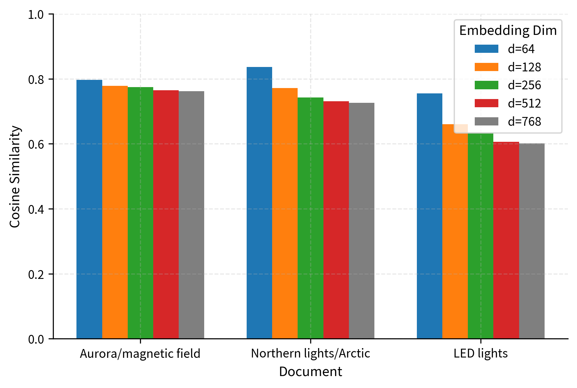
The results demonstrate the Matryoshka property nicely. Even at just 64 dimensions, the model correctly identifies the aurora/magnetic field document as most relevant. As we increase dimensions, the separation between relevant and irrelevant documents improves, and the absolute similarity scores become more calibrated. For a production system, this means you could use 128 or 256 dimensions for a fast initial retrieval pass, then use the full 768 dimensions for a more precise re-scoring, all from the same embedding model.
Key Parameters
The key parameters used in this implementation are:
- trust_remote_code: Required for models with custom architectures (like Nomic's) that are not yet part of the standard Transformers library.
- convert_to_tensor: Instructs the model to return PyTorch tensors instead of NumPy arrays, enabling efficient GPU-accelerated operations.
Embedding Model Selection
Choosing the right embedding model for your RAG pipeline is one of the highest-impact decisions you'll make. A good model makes retrieval accurate; a poor choice creates a ceiling that no amount of downstream engineering can overcome.
The MTEB Benchmark
The Massive Text Embedding Benchmark (MTEB) by Muennighoff et al. (2023) is the standard benchmark for evaluating embedding models. It covers a wide range of tasks:
- Retrieval: Finding relevant documents given a query
- Semantic Textual Similarity (STS): Scoring how similar two sentences are
- Classification: Using embeddings as features for text classification
- Clustering: Grouping similar documents together
- Pair Classification: Determining if two texts are paraphrases, entailments, etc.
- Reranking: Reordering candidate documents by relevance
- Summarization: Evaluating summary quality via embedding similarity
The MTEB leaderboard (available at huggingface.co/spaces/mteb/leaderboard) ranks models across these tasks. For RAG, the retrieval score matters most, but good performance on STS and clustering suggests the model has learned a well-organized semantic space overall.
Selection Criteria
When choosing an embedding model for a RAG system, consider these factors in rough order of importance:
-
Retrieval quality on your domain: MTEB scores are computed on general-purpose benchmarks. If you're working in a specialized domain (legal, medical, scientific), benchmark scores may not reflect actual performance. Always evaluate candidate models on a sample of your own data.
-
Language support: If your corpus includes multiple languages, you need a multilingual model. Models like
multilingual-e5-largeorbge-m3are trained on diverse language data. English-only models will fail silently on non-English text, producing embeddings that aren't meaningfully comparable. -
Context length: Standard BERT-based models handle 512 tokens. Many modern models support 8,192 tokens (like
nomic-embed-text-v1.5andgte-large-en-v1.5) or even longer. Your chunk sizes from the document chunking stage should fit within the model's context window. If your chunks exceed the model's limit, the text will be silently truncated, losing information. -
Embedding dimension and inference cost: Larger models produce better embeddings but cost more per embedding. For a corpus of 10 million documents, the difference between a 22M-parameter model and a 7B-parameter model is enormous in compute cost. Consider whether the quality improvement justifies the cost for your application.
-
Matryoshka support: If you want flexibility to trade quality for speed at serving time, or if storage costs are a concern, models with Matryoshka embeddings give you this option without retraining.
-
Instruction support: Task-aware models that accept instructions can improve retrieval quality by conditioning the embedding on the retrieval intent. This is especially useful when the same corpus is used for different types of queries.
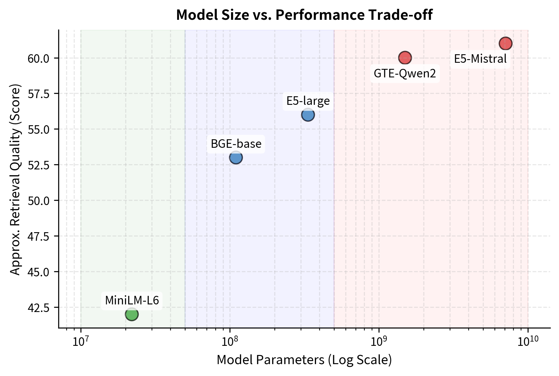
Practical Model Tiers
Based on the trade-offs above, embedding models roughly fall into three tiers for RAG applications:
-
Lightweight (< 50M parameters, 384 dimensions): Models like
all-MiniLM-L6-v2offer fast inference and small vector sizes. They're suitable for prototyping, low-resource deployments, or applications where latency matters more than peak accuracy. Encoding millions of documents is fast and cheap. -
Mid-range (100M-350M parameters, 768-1024 dimensions): Models like
bge-base-en-v1.5,gte-large-en-v1.5, ande5-large-v2represent the best trade-off for most production systems. They offer strong retrieval quality while remaining affordable to run on GPUs or even CPUs for moderate-scale corpora. -
Heavy (1B+ parameters, 1536-4096 dimensions): Models like
gte-Qwen2-1.5B-instructandE5-Mistral-7B-instructpush the quality frontier but require GPU inference and produce large vectors. They're appropriate when retrieval quality is paramount and compute budgets are generous, or when serving a smaller, high-value corpus.
Evaluating on Your Own Data
Let's walk through a practical evaluation workflow. We'll compare two models on a small retrieval task.
The high scores in this example confirm that both models successfully retrieved the relevant documents for these simple queries. This evaluation, though small, demonstrates the workflow you'd use at scale. In practice, you'd want at least 50-100 query-document pairs representative of your actual use case. The key metrics for RAG retrieval are:
- MRR (Mean Reciprocal Rank): How high does the first relevant document appear? An MRR of 1.0 means the correct document is always ranked first.
- Recall@k: What fraction of relevant documents appear in the top-k results? This directly affects RAG quality: if relevant chunks aren't retrieved, the LLM can't use them.
Key Parameters
The key parameters for SentenceTransformer models are:
- model_name_or_path: The Hugging Face model ID (e.g.,
"BAAI/bge-base-en-v1.5") or local path. - normalize_embeddings: If
Trueduring encoding, normalizes output vectors to unit length, enabling cosine similarity via dot product.
API-Based Embedding Models
Not all embedding models need to run locally. Several providers offer embedding models as API services:
- OpenAI:
text-embedding-3-small(1536 dims) andtext-embedding-3-large(3072 dims), with Matryoshka-style dimension reduction - Cohere:
embed-english-v3.0and multilingual variants, with input type parameters (search_query, search_document) - Google: Vertex AI text embeddings
- Voyage AI: Domain-specific models for code, law, and finance
API models trade control and cost predictability for convenience. For production RAG systems with large corpora, the per-token cost of API embeddings adds up. For smaller-scale or prototyping use cases, they eliminate the need to manage GPU infrastructure.
A practical concern with API embedding models is vendor lock-in: your entire vector index is tied to a specific model. If the provider deprecates the model or changes pricing, re-embedding your entire corpus can be expensive and disruptive. Open-source models you run locally avoid this risk.
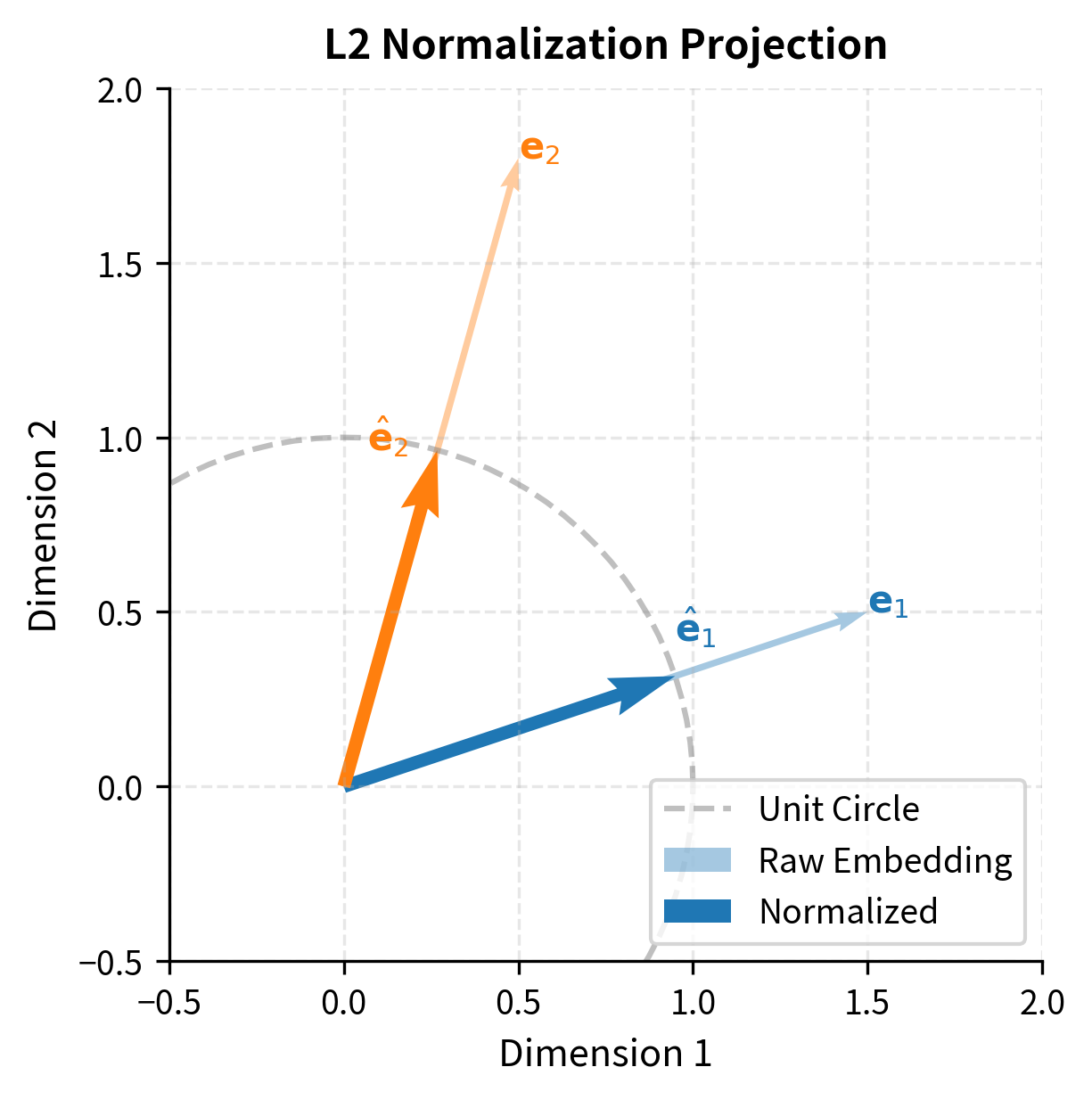
Normalization and Post-Processing
After pooling, most embedding models apply one final transformation before returning the output vector: L2 normalization. This step projects the embedding onto the surface of a unit hypersphere, ensuring that every vector has exactly the same length, regardless of the input text. The formula for this normalization divides the raw embedding by its Euclidean length:
where:
- : the L2-normalized embedding vector (unit length)
- : the raw embedding vector output by the pooling layer
- : the L2 norm (Euclidean length) of vector
To see why this matters, recall that cosine similarity between two vectors measures the cosine of the angle between them, which depends only on their direction, not their magnitude. Without normalization, two embedding vectors might differ in length for reasons unrelated to their semantic content, such as the number of tokens in the input or the distribution of activation magnitudes in the model. These length differences would complicate similarity computation because raw dot products would conflate directional similarity (which reflects semantic relatedness) with magnitude differences (which do not). By normalizing all vectors to unit length, we eliminate magnitude as a factor, ensuring that similarity measurements reflect only the angular relationship between vectors.
This normalization ensures all vectors lie on the unit hypersphere, which makes cosine similarity equivalent to the dot product:
where:
- : the normalized embedding vectors for two texts and
- : the dot product operation
This equivalence holds because the cosine similarity formula divides the dot product by the product of the two vectors' norms, and when both norms are exactly 1 (as guaranteed by L2 normalization), the denominator becomes 1, leaving just the dot product. This simplification is computationally convenient because dot products are faster to compute than cosine similarity (no need for the normalization step at search time) and are well-supported by vector index implementations. In practice, this means that once you normalize your embeddings at encoding time, you can use the simpler and faster dot product operation throughout your retrieval pipeline, without any loss of accuracy compared to cosine similarity.
Some models include a learned linear projection layer after pooling, mapping the hidden dimension to a different output dimension. For example, all-MiniLM-L6-v2 uses a hidden size of 384 and projects to 384 dimensions (identity in this case), but other models might project from 768 down to 256 to produce more compact embeddings. These projection layers are learned during training, so the model learns which linear combinations of hidden dimensions are most informative for the target embedding size. This provides another mechanism, in addition to Matryoshka training, for controlling the dimensionality of the output, though unlike Matryoshka embeddings, a fixed projection layer commits you to a single output size at inference time.
Encoding Long Documents
A practical challenge for embedding models is handling text that exceeds the model's context window. Transformers have a fixed maximum sequence length, determined by the positional encoding scheme and the memory allocated during training, and any input that exceeds this limit must be dealt with explicitly. As we discussed in the document chunking chapter, the standard approach is to split documents into chunks that fit within the model's limit. But there are alternative strategies worth knowing, each with its own trade-offs between simplicity, information preservation, and computational cost:
-
Chunked mean pooling: Encode each chunk separately, then average the resulting embeddings. This is simple but loses inter-chunk relationships. Information that spans a chunk boundary, such as a sentence that begins in one chunk and concludes in the next, is split across two embeddings and cannot be fully captured by either.
-
Hierarchical encoding: Produce chunk-level embeddings, then use a separate aggregation model to combine them into a document embedding. This approach can potentially capture inter-chunk relationships if the aggregation model is expressive enough, but it adds complexity and a second model to the pipeline.
-
Long-context embedding models: Some newer models (like
jina-embeddings-v2-base-enwith 8192 tokens) natively handle longer sequences, reducing the need for aggressive chunking. These models use modified positional encoding schemes, such as ALiBi or RoPE with extended context, to process inputs many times longer than the original BERT limit of 512 tokens.
For RAG applications, per-chunk embeddings are almost always preferable to document-level embeddings. When you ask a specific question, you want to retrieve the specific chunk that answers it, not an entire document that might bury the relevant passage among thousands of irrelevant tokens. A document-level embedding must somehow represent the meaning of the entire document in a single vector, and this extreme compression makes it difficult to match precise, narrowly focused queries. Chunk-level embeddings, by contrast, each represent a smaller, more focused unit of content, making it far more likely that a relevant chunk will be retrieved for a specific question.
Limitations and Practical Considerations
Embedding models, despite their impressive capabilities, have important limitations that affect RAG system design. The most fundamental is the information bottleneck: compressing a passage of potentially hundreds of tokens into a single fixed-length vector inevitably loses information. A 768-dimensional vector simply cannot encode every nuance of a 512-token passage. This is why cross-encoder rerankers, which we'll discuss later in this part, can improve accuracy by performing full token-level cross-attention between the query and each candidate document.
Another significant limitation is domain mismatch. General-purpose embedding models are trained primarily on web text, Wikipedia, and common NLP benchmarks. When deployed on specialized domains (medical literature, legal contracts, codebases, financial reports), their performance can drop substantially. The embedding space may not have learned the fine-grained distinctions that matter in your domain. For example, a general model might place "myocardial infarction" and "cardiac arrest" close together because they're both heart-related, even though they're clinically distinct conditions. Domain-specific fine-tuning with contrastive learning on in-domain pairs can address this, but it requires labeled data and training infrastructure.
There's also the issue of embedding drift over time. If your corpus evolves (new documents are added, existing ones are updated), and you switch to a new embedding model version, all previously computed embeddings become incompatible. You cannot mix embeddings from different models in the same vector index. This means model upgrades require re-embedding the entire corpus, which can be a multi-day operation for large-scale systems.
Finally, embedding models inherit the biases present in their training data. If certain topics, perspectives, or demographics are underrepresented in training, the embedding space will be poorly calibrated for those inputs. Queries from underrepresented groups or about underrepresented topics may receive lower-quality retrieval results, an important consideration for equitable information access.
Summary
This chapter covered the architecture and design decisions that make embedding models work for retrieval in RAG systems:
- Embedding models are transformer encoders fine-tuned with contrastive objectives to produce semantically meaningful sentence and passage vectors. They bridge the gap between token-level transformer outputs and the single-vector representations needed for retrieval.
- Pooling strategies determine how token embeddings are compressed into a single vector. Mean pooling is the most common and effective for encoder models, while last token pooling is used for decoder-based embedding models. The pooling strategy must match what the model was trained with.
- Embedding dimensionality involves a trade-off between representational capacity and computational cost. Most production systems use 384 to 1024 dimensions. Matryoshka representation learning allows flexible dimensionality from a single model.
- Model selection should be guided by retrieval performance on your specific data, not just benchmark scores. Consider language support, context length, inference cost, and the risk of vendor lock-in.
- Normalization to unit length simplifies cosine similarity to dot product, enabling faster search and compatibility with standard vector index implementations.
With embeddings in hand, the next step in a RAG pipeline is storing them in a way that enables fast similarity search. The upcoming chapters on vector similarity search, HNSW, and IVF indices will show how to search over millions of vectors without resorting to brute-force comparison.
Quiz
Ready to test your understanding? Take this quick quiz to reinforce what you've learned about embedding models.

Comments