

Master dense retrieval for semantic search. Explore bi-encoder architectures, embedding metrics, and contrastive learning to overcome keyword limitations.

This article is part of the free-to-read Language AI Handbook
Choose your expertise level to adjust how many terms are explained. Beginners see more tooltips, experts see fewer to maintain reading flow. Hover over underlined terms for instant definitions.
Dense Retrieval
In the previous chapter, we examined the RAG architecture and how it combines retrieval with generation. At the heart of this system lies a critical question: how do we find the most relevant documents for a given query? Traditional search engines rely on lexical matching, counting how often query terms appear in documents. But what if the document uses different words to express the same concept? What if "automobile" appears in the document but you search for "car"?
Dense retrieval addresses this fundamental limitation by representing both queries and documents as continuous vectors in a shared semantic space. Rather than matching exact words, dense retrieval measures the similarity between the meanings of queries and documents. A query about "climate change impacts" can match documents discussing "global warming effects" because both map to nearby points in the embedding space, even though they share no common terms.
This shift from discrete term matching to continuous semantic similarity is a significant advance in information retrieval. Building on the transformer architectures and embedding techniques we've explored throughout this book, dense retrieval enables retrieval systems that understand language rather than merely counting words.
From Lexical to Semantic Matching
Recall from Part II that BM25 retrieves documents by computing term-frequency statistics: documents score higher when they contain more query terms, with diminishing returns for repeated terms and penalties for common words. This approach works remarkably well for many queries, but it fails when queries and relevant documents use different vocabulary.
Consider searching a medical knowledge base with the query "heart attack symptoms." A relevant document might discuss "myocardial infarction warning signs" without ever using the words "heart" or "attack." BM25 would score this document at zero because it shares no terms with the query. Yet a physician would recognize these as describing the same condition.
This vocabulary mismatch problem becomes acute in several scenarios:
- Synonyms and paraphrases: "car" vs "automobile," "purchase" vs "buy"
- Technical vs casual language: "myocardial infarction" vs "heart attack"
- Abbreviations and expansions: "ML" vs "machine learning"
- Conceptual similarity: "renewable energy policy" might relate to documents about "solar panel subsidies"
Dense retrieval sidesteps vocabulary mismatch entirely. Instead of asking "which words match?", it asks "which meanings match?" By encoding both queries and documents into a continuous vector space where semantically similar texts cluster together, dense retrieval can find relevant documents regardless of the specific words they use.
The Bi-Encoder Architecture
The dominant architecture for dense retrieval is the bi-encoder, which uses two separate encoder networks to produce embeddings for queries and documents independently. This separation is crucial for efficiency at scale, and understanding why requires us to think carefully about what happens during retrieval.
A neural architecture that encodes queries and documents using separate (but often identical) transformer encoders, producing fixed-dimensional vectors that can be compared using simple similarity metrics.
Architecture Overview
The bi-encoder consists of two components that work in tandem to transform text into comparable numerical representations. The first component is the query encoder, denoted , which takes a natural language query as input and produces a dense vector representation. The second component is the document encoder, denoted , which performs the analogous transformation for documents.
Formally, we can express these transformations as follows:
- Query encoder : Maps a query to a dense vector
- Document encoder : Maps a document to a dense vector
Both encoders are typically initialized from the same pre-trained transformer (such as BERT, as we covered in Part XVII), and they may share weights or be fine-tuned independently. The encoders produce embeddings of the same dimensionality , enabling direct comparison. This shared dimensionality is essential because it allows us to measure distances and angles between query and document vectors in the same geometric space.
A key challenge in building these encoders is converting the variable-length output of a transformer into a single fixed-size vector suitable for comparison. Recall that when a BERT model processes an input sequence, it produces a hidden state vector for each token in the sequence. To condense this sequence of token representations into a single fixed-size vector, BERT-based encoders typically extract the representation of the special [CLS] token from the final layer:
where:
- is the dense vector representation of the query
- is the sequence of hidden states from the last layer of the BERT model
- indicates extraction of the vector corresponding to the special classification token (designed to aggregate sequence-level information)
Alternatively, to capture information distributed across the entire sequence rather than relying on a single token, some models compute the average of all token representations. This approach, known as mean pooling, treats each token's contribution equally:
where:
- is the dense vector representation of the query
- is the number of tokens in the query
- is the vector representation of the -th token
- computes the element-wise sum of all token vectors to find the geometric center
The intuition behind mean pooling is that important semantic information may be spread across multiple tokens rather than concentrated in the [CLS] token. By averaging, we create a representation that balances contributions from all parts of the input. The choice between [CLS] pooling and mean pooling affects retrieval quality, and different models adopt different strategies based on their training objectives. Empirically, models trained with mean pooling as part of their objective tend to perform better when evaluated using mean pooling, and likewise for [CLS] pooling.
Why Separate Encoders?
The bi-encoder's separation of query and document encoding enables a critical optimization: pre-computation of document embeddings. To appreciate why this matters, consider the computational demands of a retrieval system. In a retrieval system with millions of documents, we can encode all documents offline, storing their embeddings in a vector index. At query time, we only need to encode the query once, then compare it against the pre-computed document embeddings.
This contrasts with cross-encoders, which concatenate the query and document and process them jointly through a single transformer. Cross-encoders can capture fine-grained interactions between query and document tokens, often achieving higher accuracy, but they require running the transformer once for every query-document pair. For a corpus of 10 million documents, this means 10 million transformer forward passes per query, which is computationally infeasible.
The bi-encoder architecture trades some modeling power for massive efficiency gains:
| Aspect | Bi-Encoder | Cross-Encoder |
|---|---|---|
| Query-time computation | Encode query once | Encode query-doc pairs |
| Document pre-computation | Yes (offline) | No |
| Query-document interaction | None (independent encoding) | Full attention |
| Typical use | First-stage retrieval | Reranking |
| Scalability | Millions of documents | Hundreds of candidates |
We'll explore reranking with cross-encoders in a later chapter, where they serve as a second-stage refinement over bi-encoder candidates.
Embedding Similarity Metrics
Once we have query and document embeddings, we need a similarity function to rank documents. The three most common metrics are dot product, cosine similarity, and Euclidean distance. Each of these metrics captures a different notion of what it means for two vectors to be "similar," and understanding their geometric interpretations helps us choose the right metric for a given application.
Dot Product
The dot product quantifies the similarity between two vectors by aggregating their aligned components. To understand this intuitively, imagine two vectors as arrows pointing in some direction in high-dimensional space. The dot product measures how much one vector "projects" onto another, combining information about both their directions and their lengths. For vectors and , the dot product is defined as:
where:
- is the similarity score
- are the dense vectors for the query and document
- is the dimensionality of the embedding space (e.g., 768)
- are the -th scalar components
- aggregates alignment across all dimensions
The geometric interpretation of this formula is instructive. Each dimension of the embedding space captures some aspect of meaning. When both and are large and positive, their product contributes positively to the similarity, indicating that both the query and document exhibit that particular semantic feature strongly. Conversely, when one is positive and the other negative, the contribution is negative, reducing overall similarity.
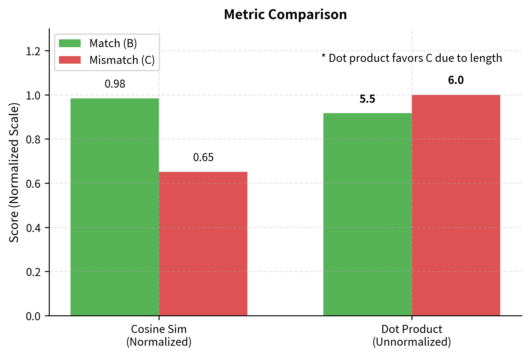
The dot product is computationally efficient and captures both the alignment of vectors (their angular similarity) and their magnitudes. Larger embeddings produce larger dot products, which can be useful when magnitude carries semantic meaning. For example, longer, more detailed documents might have larger embedding norms, and this property could be desirable if we want to favor comprehensive documents.
Many dense retrieval models, including DPR (Dense Passage Retrieval), use dot product similarity because it can be computed extremely efficiently using matrix multiplication. Given a query vector and a matrix of document vectors, we can compute all similarity scores in a single operation, leveraging highly optimized linear algebra libraries.
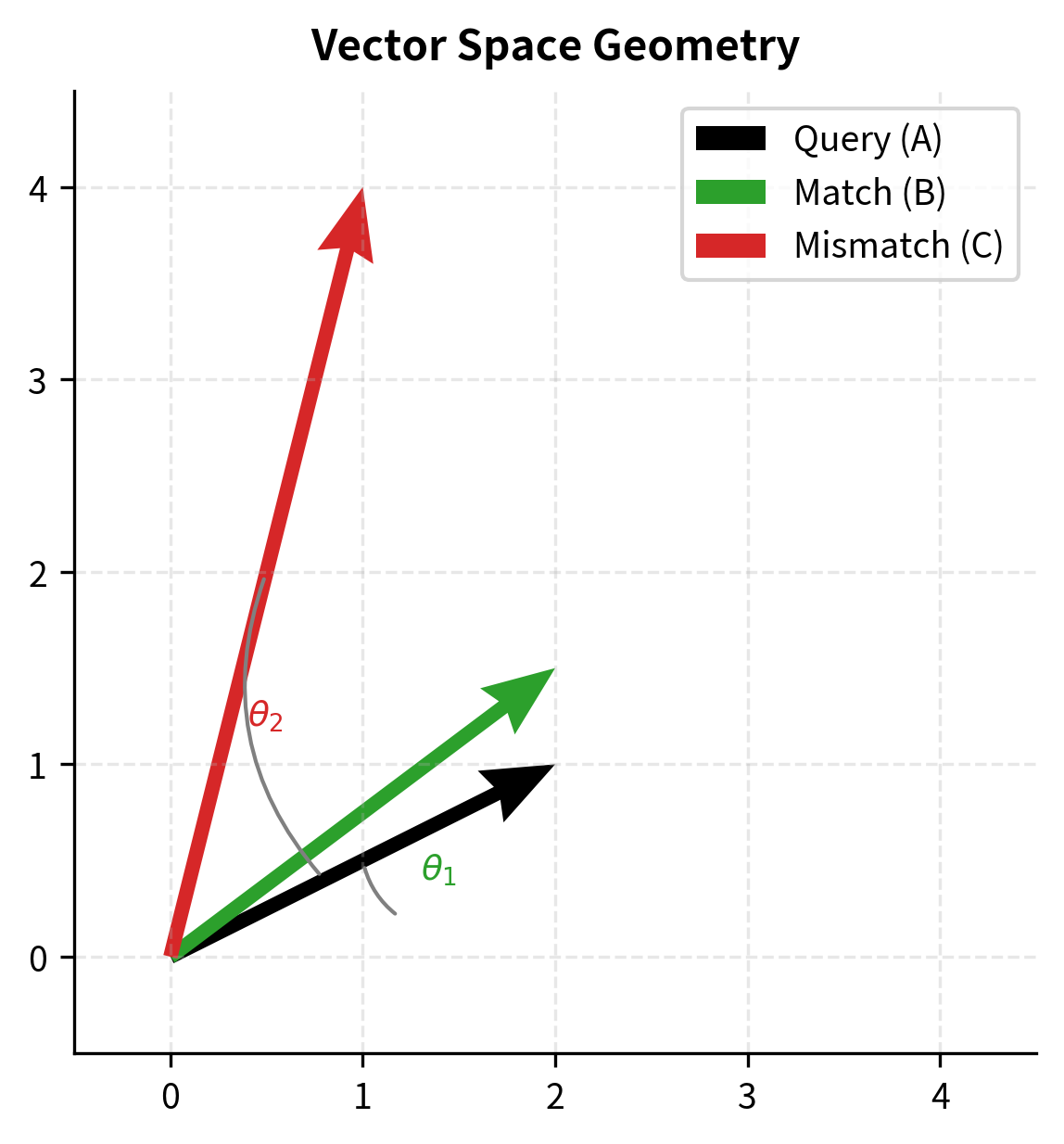
Cosine Similarity
While the dot product captures both direction and magnitude, there are situations where we want to focus purely on semantic direction, ignoring how "long" the vectors are. Cosine similarity addresses this need by normalizing the dot product by the magnitudes of both vectors, measuring only the angular alignment:
where:
- is the cosine similarity score
- is the dot product (unnormalized projection)
- are the Euclidean norms (lengths) of the vectors
- calculates the vector magnitude
The cosine similarity ranges from (opposite directions) to (same direction), with indicating orthogonality, meaning the vectors are perpendicular in the embedding space. By removing magnitude effects, cosine similarity focuses purely on semantic direction. This is particularly useful when we want to compare texts of different lengths on an equal footing, since a longer document might naturally produce a larger-magnitude embedding without being more relevant.
A useful property emerges when embeddings are L2-normalized, meaning each vector is divided by its magnitude so that . In this case, cosine similarity equals the dot product:
Here, and are the unit-length vectors derived by dividing and by their respective norms. The dot product operation, applied to these normalized vectors, now directly yields the cosine of the angle between the original vectors.
This equivalence is useful because we can pre-normalize all document embeddings and use the faster dot product operation while still computing cosine similarity. This is exactly what many production systems do: they normalize embeddings once during indexing, then use simple dot products during retrieval.
Euclidean Distance
The third common metric takes a different perspective entirely. Rather than measuring how vectors align, Euclidean (L2) distance measures the straight-line distance between vectors in the embedding space:
where:
- is the Euclidean distance
- is the difference vector
- is the squared difference in dimension
- converts the sum of squared differences to linear distance
Unlike the similarity metrics above, smaller distances indicate greater similarity. This is an important distinction to keep in mind when implementing retrieval systems: with Euclidean distance, we search for the nearest neighbors rather than the highest-scoring documents.
Euclidean distance is related to dot product for normalized vectors. When vectors have unit length, minimizing Euclidean distance is mathematically equivalent to maximizing the dot product. This relationship allows certain indexing algorithms designed for one metric to be adapted for the other.
Choosing a Metric
The choice of similarity metric should match the training objective used when the embedding model was created:
- Models trained with dot product loss perform best with dot product similarity
- Models trained with cosine loss perform best with cosine similarity
- Many embedding models normalize their outputs, making the choice less critical
In practice, cosine similarity (or equivalently, dot product with normalized embeddings) is the most common choice because it's robust to variations in embedding magnitude and provides easily interpretable scores. When similarity ranges from 0 to 1, it becomes straightforward to set thresholds and compare scores across different queries.
Dense vs Sparse Retrieval: A Detailed Comparison
Understanding when to use dense versus sparse retrieval requires examining their complementary strengths and weaknesses.
Strengths of Dense Retrieval
Dense retrieval excels in scenarios where semantic understanding matters more than exact term matching:
Semantic matching: Dense retrieval captures meaning beyond surface forms. The query "best laptop for programming" matches documents about "developer-friendly notebooks with good keyboards" even without shared terms.
Handling synonyms: Medical queries like "hypertension treatment" naturally match documents about "high blood pressure medication" because both concepts map to similar regions in the embedding space.
Cross-lingual retrieval: With multilingual encoders, the same query can retrieve relevant documents in different languages, as semantically equivalent text in different languages clusters together in the embedding space.
Robustness to typos: Minor spelling variations ("recieve" vs "receive") often produce similar embeddings, whereas exact-match systems would fail entirely.
Strengths of Sparse Retrieval
Sparse retrieval (BM25, TF-IDF) maintains advantages in several areas:
Exact match requirements: When you search for specific identifiers like "CVE-2024-1234" or "iPhone 15 Pro Max," exact term matching is essential. Dense models may confuse similar but distinct identifiers.
Rare terms and proper nouns: Uncommon terms carry high information value in BM25 (high IDF weights). Dense models may underweight rare terms that weren't well-represented in training data.
Interpretability: BM25 scores are explainable: "this document ranked high because it contains the query terms 'machine' (3 times) and 'learning' (5 times)." Dense similarity scores are opaque.
Zero-shot generalization: BM25 works immediately on any corpus without training. Dense retrievers need training data that matches the target domain.
Efficiency: BM25 uses inverted indices that scale efficiently to billions of documents. Dense retrieval requires vector indices that are more memory-intensive.
When Each Approach Fails
Dense retrieval struggles with:
- Keyword-heavy queries: Searching for "Python pandas DataFrame merge" requires exact library and function names
- Out-of-domain text: Models trained on Wikipedia may perform poorly on legal contracts
- Negation: "hotels without pools" might match documents about "hotels with pools" because both contain similar concepts
- Numerical reasoning: 'apartments under \$2000/month' requires understanding numerical constraints
Sparse retrieval struggles with:
- Vocabulary mismatch: "affordable housing" vs "low-cost apartments"
- Paraphrased queries: "what causes climate change" vs "global warming factors"
- Conceptual queries: "books like Harry Potter" requires understanding genre and style
- Short queries: Single-word queries provide little context for term weighting
The Case for Hybrid Approaches
Given these complementary strengths, many production systems combine both approaches. A typical hybrid strategy:
- Run both dense and sparse retrieval in parallel
- Normalize scores from each system
- Combine scores with learned or tuned weights
- Return the top-k documents from the merged ranking
We'll explore hybrid search techniques in detail in a later chapter on combining retrieval signals.
Training Dense Retrievers
Creating effective dense retrievers requires specialized training to produce embeddings where similar queries and documents cluster together. This section covers the key components of the training process, from the mathematical objective that guides learning to the practical considerations of data collection and negative sampling.
The Training Objective
The goal of dense retriever training is to learn an embedding space where:
- Relevant query-document pairs have high similarity
- Irrelevant query-document pairs have low similarity
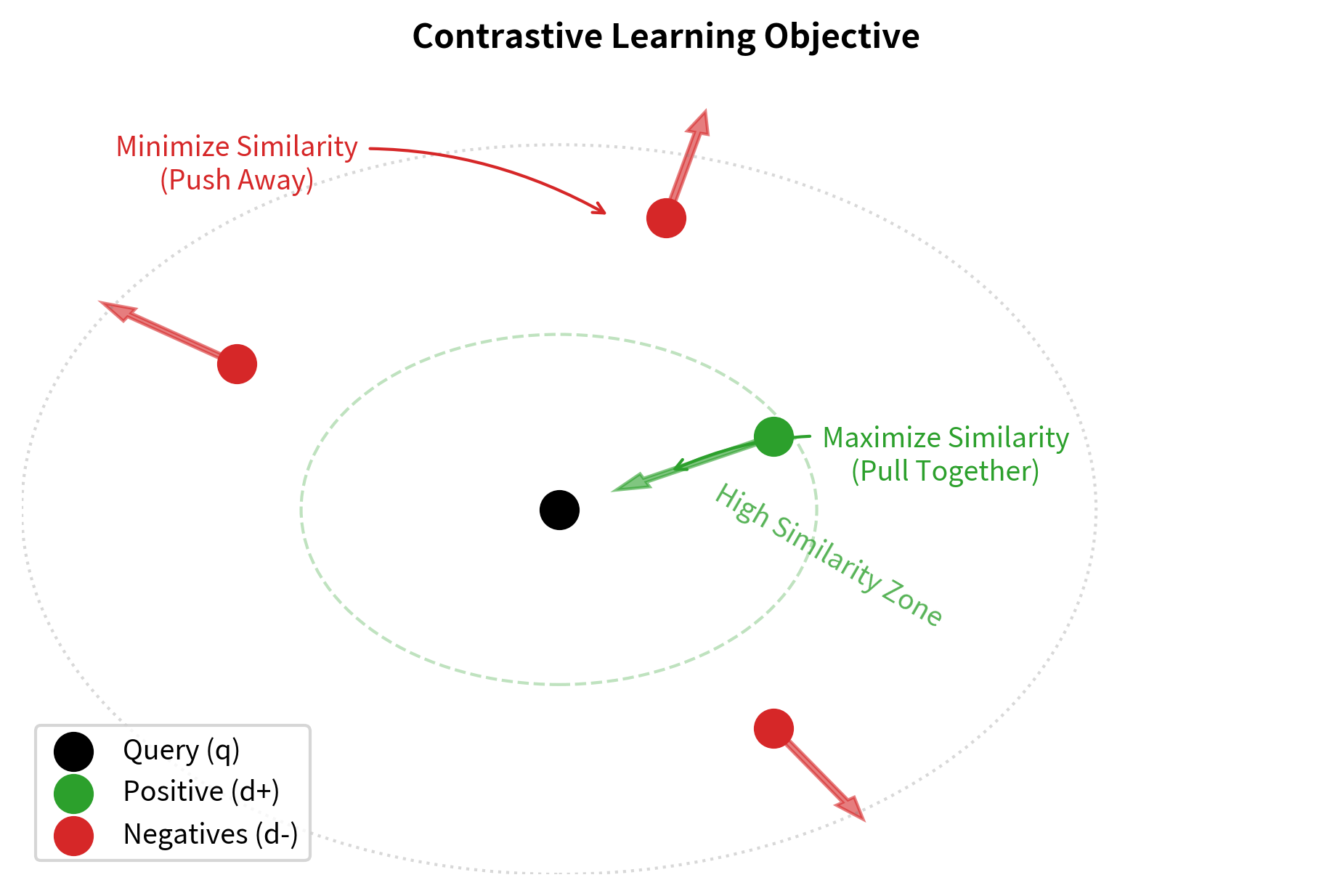
This is typically formulated as a contrastive learning problem. The core idea is deceptively simple: teach the model to distinguish between documents that satisfy your information need and documents that do not. Given a query , a relevant (positive) document , and irrelevant (negative) documents , we want:
where:
- is the similarity function (e.g., dot product)
- are the encoder embeddings
- is the relevant (positive) document
- is the -th irrelevant (negative) document
- indicates the condition holds for all negative samples
The intuition behind this formulation is geometric: we want the query embedding to be closer to the positive document embedding than to any negative document embedding in the vector space.
The most common loss function is the contrastive loss (also called InfoNCE loss). This function treats retrieval as a classification task. It first computes the probability that the positive document is the correct match among the set of negatives, then minimizes the negative log of that probability. The mathematical formulation is:
where:
- is the probability that is the correct match
- is the loss to minimize
- are the embeddings for query, positive, and negative docs
- is the temperature parameter
- is the number of negative samples
The temperature parameter controls the sharpness of the probability distribution and deserves special attention. When is small (close to 0), the exponential function amplifies differences between similarity scores, making the model more confident in its distinctions. When is large, the probability distribution becomes more uniform, making the training signal weaker. Finding the right temperature is often done through experimentation.
In the numerator, computes the exponential score for the positive pair. In the denominator, sums the exponential scores for all negative samples. Combined with the positive pair's score, this sum forms the normalization constant that ensures probabilities sum to one.
This loss pushes the model to increase the similarity between query and positive document while decreasing similarity with negatives. We'll explore contrastive learning in much greater depth in the next chapter.
Training Data Sources
Dense retrievers require training data consisting of query-document pairs with relevance labels. Common sources include:
Natural Questions (NQ): Google's dataset of real questions paired with Wikipedia passages containing answers. This provides natural query distribution but limited to Wikipedia domain.
MS MARCO: Microsoft's large-scale reading comprehension dataset with web queries and relevant passages. Its scale (500k+ queries) and web domain make it popular for training general-purpose retrievers.
Synthetic data: Using LLMs to generate queries for existing documents. Given a passage, the model generates questions that the passage would answer. This allows creating training data for any domain.
Click logs: In production systems, your clicks provide implicit relevance signals. Documents that you click after a query are treated as positive examples.
Negative Sampling Strategies
The choice of negative documents significantly impacts training quality. Several strategies exist:
Random negatives: Sample random documents from the corpus. Simple but often too easy: random documents are typically obviously irrelevant.
BM25 negatives: Use BM25 to find documents that match query terms but aren't relevant. These "hard negatives" share surface features with the query but differ semantically, forcing the model to learn beyond lexical overlap.
In-batch negatives: Use positive documents from other queries in the same training batch as negatives. Efficient because it requires no additional encoding, but the negatives may be too easy.
Self-mined hard negatives: Use the current model to find high-scoring documents that aren't labeled as relevant. These are the hardest negatives because the current model finds them confusable with true positives.
Research has shown that combining these strategies often works best: start with random negatives for initial training, then fine-tune with BM25 and self-mined hard negatives.
The Training Pipeline
A typical dense retriever training pipeline:
- Initialize query and document encoders from pre-trained BERT
- Construct batches with queries, positive documents, and sampled negatives
- Encode all queries and documents in the batch
- Compute pairwise similarities and contrastive loss
- Backpropagate through both encoders
- Repeat for multiple epochs, potentially re-mining hard negatives periodically
The training process is computationally intensive because we need to encode many negatives per query to provide a strong training signal. Techniques like in-batch negatives help by reusing computation across the batch.
Worked Example: Semantic Similarity in Action
Let's trace through a concrete example to build intuition for how dense retrieval differs from lexical matching. This example will help cement the abstract concepts we've discussed by showing them in operation on real text.
Consider a query and three candidate documents:
Query: "How do plants make food?"
Document A: "Photosynthesis is the process by which green plants and certain other organisms transform light energy into chemical energy."
Document B: "Plants require sunlight, water, and carbon dioxide to produce glucose and oxygen through a complex series of reactions."
Document C: "My grandmother makes delicious food using fresh vegetables from her garden."
From a BM25 perspective, Document C contains both "plants" (via "vegetables" and "garden" context) and "food," giving it some term overlap with the query. Documents A and B share no direct terms with "How do plants make food?" This illustrates the vocabulary mismatch problem: the most relevant documents use technical terminology ("photosynthesis," "glucose," "chemical energy") that doesn't appear in your natural language query.
A dense retriever, however, produces embeddings that capture semantic meaning rather than surface-level word matches:
- Query embedding: Encodes the concept of "plant nutrition/energy production"
- Document A embedding: Clusters near "plant biology, photosynthesis" concepts
- Document B embedding: Also clusters near "plant biology, photosynthesis"
- Document C embedding: Clusters near "cooking, family, gardening" concepts
The cosine similarity between query and Document A might be 0.78, between query and Document B might be 0.75, while query and Document C might be only 0.21. Despite Document C's lexical overlap, its semantic meaning is far from the query's intent. The dense retriever recognizes that "making food" in the context of plants refers to biological energy production, not culinary preparation.
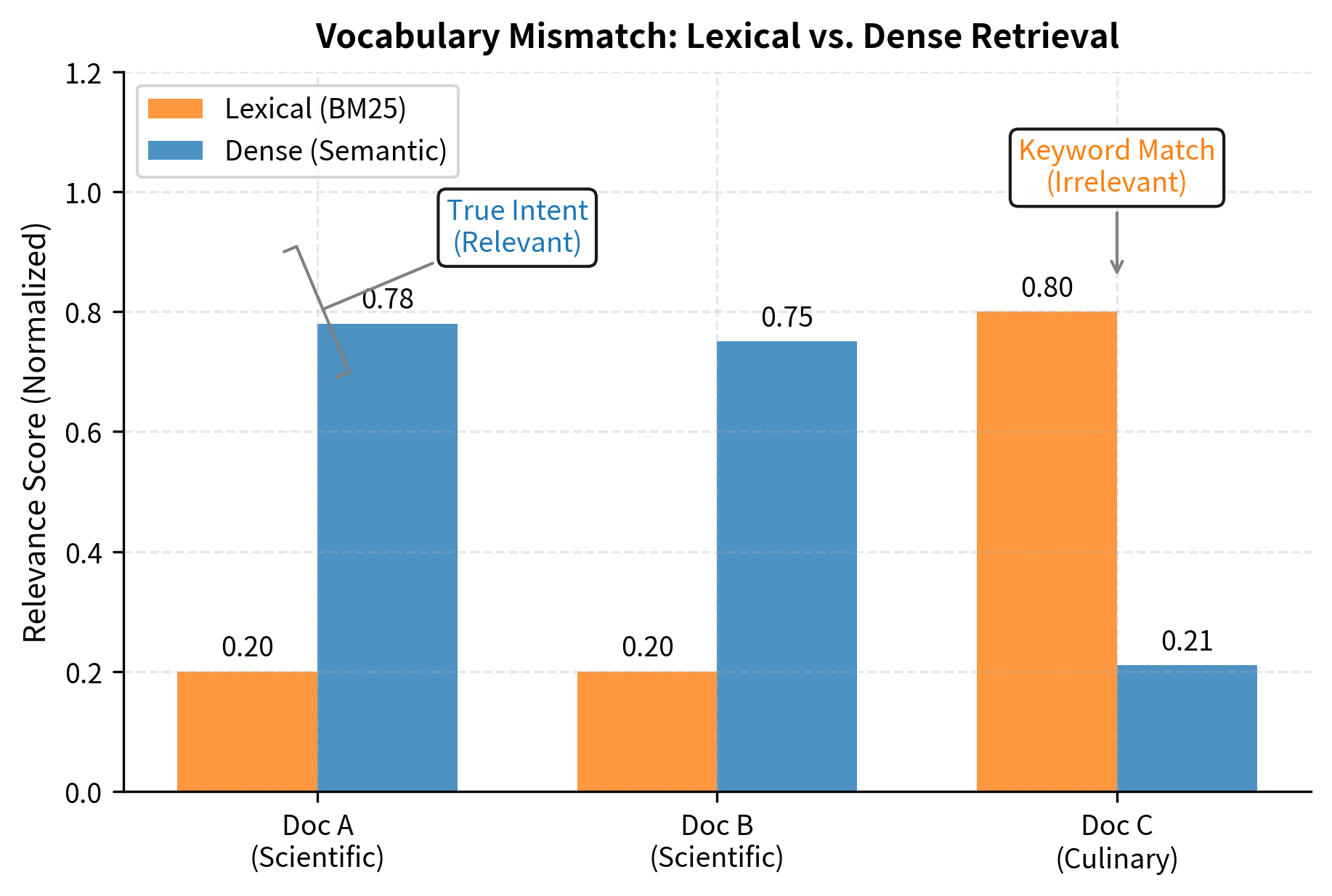
This example illustrates the fundamental difference: sparse retrieval operates on surface forms, counting which words appear and how often, while dense retrieval operates on underlying meaning, measuring conceptual similarity in a learned semantic space.
Code Implementation
Let's implement dense retrieval using the sentence-transformers library, which provides pre-trained bi-encoder models optimized for semantic similarity.
The all-MiniLM-L6-v2 model is a compact but effective retriever, producing 384-dimensional embeddings. It was trained on over 1 billion sentence pairs using contrastive learning.
Each document is now represented as a 384-dimensional vector. In a production system, these embeddings would be stored in a vector index for efficient search.
Computing Similarity Scores
Let's implement a function to retrieve documents for a query:
Let's test our retriever with a query that demonstrates semantic matching:
The retriever finds documents about neural network learning, gradient descent (the mechanism for learning), and backpropagation (how gradients are computed). These are semantically related to the query even when they don't contain the exact query terms.
Comparing Dense and Lexical Retrieval
Let's compare dense retrieval to a simple lexical approach:
Now let's test both approaches on a query with vocabulary mismatch:
Dense retrieval finds semantically relevant documents about gradient descent and neural network learning, while simple lexical matching struggles because the query terms don't appear in the documents. This demonstrates the vocabulary mismatch problem that dense retrieval addresses.
Visualizing the Embedding Space
Let's visualize how documents cluster in the embedding space:
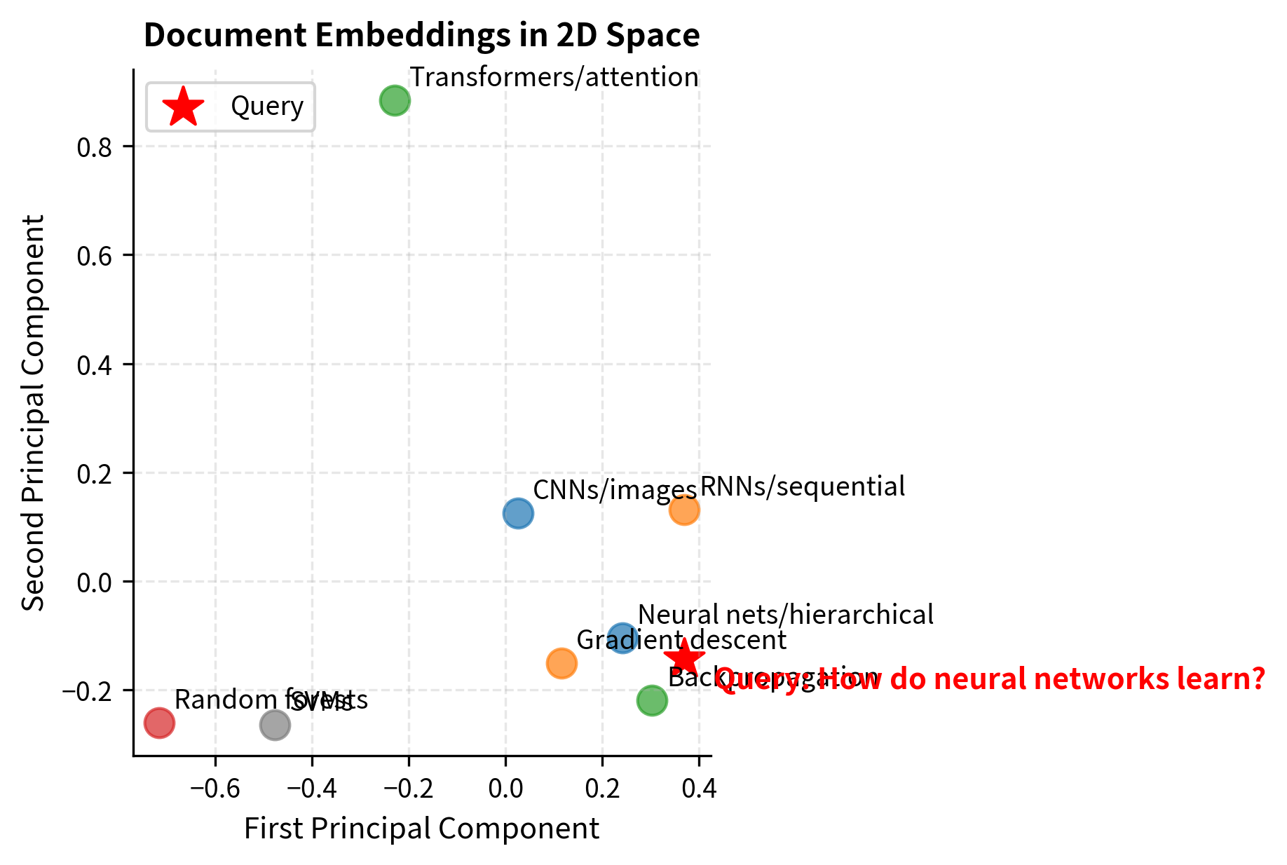
The visualization shows how documents cluster by topic in the embedding space. The query "How do neural networks learn?" is positioned near documents about neural networks, gradient descent, and backpropagation, enabling semantic retrieval without term matching.
Batch Retrieval for Efficiency
In practice, we encode multiple queries at once for efficiency:
The matrix multiplication computes all query-document similarities simultaneously, making batch retrieval much more efficient than processing queries one at a time.
Key Parameters
The key parameters for the Dense Retrieval implementation are:
- model_name_or_path: Argument for
SentenceTransformerto select the pre-trained weights (e.g.,'all-MiniLM-L6-v2'). Different models offer different trade-offs between speed, model size, and embedding quality. - normalize_embeddings: Argument for
model.encode. When set toTrue, it produces unit-length vectors, enabling dot product to equal cosine similarity. - top_k: Argument for the retrieval function determining the number of results to return. In a RAG pipeline, this controls context size.
Limitations and Impact
Dense retrieval has transformed information retrieval, but understanding its limitations is essential for effective deployment.
Key Limitations
Dense retrievers require substantial training data to perform well. Unlike BM25, which works out-of-the-box on any text collection, dense models need labeled query-document pairs that match the target domain. A retriever trained on Wikipedia passages may perform poorly on legal contracts, scientific papers, or code documentation. This domain sensitivity means organizations often need to fine-tune models on their specific data, which requires expertise and labeled examples.
The computational requirements of dense retrieval are significant. Each document must be encoded by a transformer model, and the resulting embeddings must be stored and indexed. For a corpus of 100 million documents with 384-dimensional embeddings, storage alone requires approximately 150 gigabytes. Sparse indices based on inverted lists often require far less memory and can be searched faster for simple keyword queries. The next chapters on vector similarity search and indexing techniques address how to make dense retrieval practical at scale.
Dense retrievers can also fail silently in ways that sparse retrievers don't. When BM25 returns poor results, the explanation is often clear: the query terms don't appear in relevant documents. When a dense retriever fails, diagnosing the problem is harder. The model might not have learned good representations for certain concepts, might confuse similar-sounding but different entities, or might not handle negation correctly. This opacity makes debugging and improving dense retrieval systems more challenging.
Impact on NLP Systems
Despite these limitations, dense retrieval has had enormous impact. By enabling semantic matching at scale, it unlocked new capabilities across NLP:
Question answering systems improved dramatically when they could retrieve passages by meaning rather than keywords. Open-domain QA, where systems answer questions using large document collections, became practical with dense retrieval.
RAG systems, which we introduced in the previous chapters, depend critically on dense retrieval. The ability to find semantically relevant passages allows LLMs to answer questions about current events, specialized domains, and private data that wasn't in their training set.
Semantic search products from Google, Microsoft, and others now incorporate dense retrieval, improving results for conversational queries and complex information needs.
Cross-lingual applications became more practical because dense models can encode meaning across languages, enabling search systems where queries and documents may be in different languages.
The combination of transformer pre-training and contrastive learning for retrieval, which we'll explore in the next chapter, established the foundation for modern semantic search systems.
Summary
Dense retrieval represents a fundamental shift from lexical to semantic matching in information retrieval. Rather than counting term overlaps, dense retrievers encode queries and documents into continuous vector spaces where similarity reflects semantic relatedness.
The bi-encoder architecture enables scalable dense retrieval by separating query and document encoding. Documents can be pre-computed and indexed offline, requiring only a single query encoding at search time. This efficiency trade-off sacrifices some of the fine-grained interaction captured by cross-encoders but enables retrieval over millions of documents.
Embedding similarity metrics, particularly cosine similarity and dot product, quantify semantic relatedness between query and document vectors. The choice of metric should align with the model's training objective, though many models normalize embeddings, making the metrics equivalent.
Dense and sparse retrieval have complementary strengths. Dense retrieval excels at semantic matching and handles vocabulary mismatch gracefully, while sparse retrieval provides exact term matching, better handles rare terms, and offers more interpretable results. Production systems often combine both approaches in hybrid architectures.
Training dense retrievers requires query-document pairs and careful negative sampling. The contrastive learning objective pushes the model to maximize similarity between relevant pairs while minimizing similarity with hard negatives. The quality of negatives significantly impacts the learned embedding space.
In the next chapter, we'll dive deeper into contrastive learning for retrieval, examining the training objectives, loss functions, and techniques that produce effective dense retrieval models.
Quiz
Ready to test your understanding? Take this quick quiz to reinforce what you've learned about dense retrieval and semantic matching.

Comments