

Master contrastive learning for dense retrieval. Learn to train models using InfoNCE loss, in-batch negatives, and hard negative mining strategies effectively.

This article is part of the free-to-read Language AI Handbook
Choose your expertise level to adjust how many terms are explained. Beginners see more tooltips, experts see fewer to maintain reading flow. Hover over underlined terms for instant definitions.
Contrastive Learning for Retrieval
In the previous chapter, we introduced dense retrieval and the idea of encoding queries and passages into a shared embedding space where relevance is measured by vector similarity. But we left a critical question unanswered: how do you actually train encoders to place relevant query-passage pairs close together and irrelevant ones far apart?
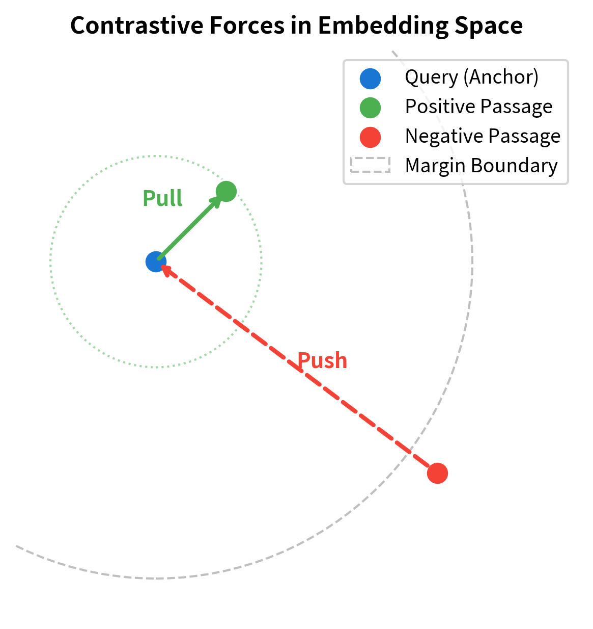
The answer is contrastive learning, a training paradigm built around a simple idea: teach a model what things should look like together by also showing it what things should not look like together. Rather than predicting labels or generating text, a contrastive model learns to distinguish positive pairs (a query matched with its relevant passage) from negative pairs (a query matched with irrelevant passages). The loss function rewards the model for increasing the similarity of positive pairs while decreasing the similarity of negatives.
This idea has roots we've seen before. Recall from Part IV that negative sampling in Word2Vec works on a similar principle: the skip-gram model learns word embeddings by distinguishing true context words from randomly sampled negative words. Contrastive learning for retrieval extends this concept to full sequences, using BERT-style encoders instead of lookup tables and operating over passages rather than individual words.
In this chapter, we'll build up the contrastive learning framework piece by piece. We start with the core loss function, then examine two techniques that make training practical and effective: in-batch negatives (which give you hundreds of negatives "for free") and hard negative mining (which provides the challenging examples a model needs to learn fine-grained distinctions). We'll then walk through the complete training procedure of Dense Passage Retrieval (DPR), the model that brought these ideas together into a system that outperformed BM25 on open-domain question answering.
The Contrastive Learning Framework
Contrastive learning is a form of metric learning. Instead of training a model to output a class label or predict the next token in a sequence, you train it to produce representations where a distance or similarity metric reflects the semantic relationship between inputs. The core philosophy is that you do not tell the model what something means in isolation; rather, you tell the model how things relate to each other, and you do so by showing both positive and negative examples of those relationships. For retrieval, this translates into a concrete objective: given a query and a relevant passage , their embeddings should have high similarity, while a query and an irrelevant passage should have low similarity.
This framing sidesteps the need for explicit labels that describe what a passage is "about." You never need to assign a topic tag or a relevance score on a fixed scale. Instead, you only need to specify pairwise relationships: this query goes with this passage, and not with that one. The model's internal representations emerge organically from the pressure of having to satisfy many such relational constraints simultaneously.
The training data for contrastive retrieval consists of pairs where each query is associated with at least one known relevant passage. These positive pairs might come from various sources:
- Question-answer datasets: The passage containing the answer is the positive for that question.
- Click logs: A document that you clicked after issuing a search query.
- Hyperlinks: The anchor text serves as a "query" and the linked page as the positive passage.
- Manual annotations: Human judges label query-document relevance.
Each of these sources carries different biases and varying levels of noise. Click logs are plentiful but noisy, since you sometimes click on irrelevant documents. Manual annotations are high-quality but expensive to collect at scale. Question-answer datasets offer a middle ground, providing naturally occurring query-passage pairs where relevance is clearly defined by whether the passage contains the answer. Regardless of the source, the fundamental structure is the same: pairs of inputs that should end up close together in the learned embedding space.
The key challenge is that we also need negative examples, passages that are irrelevant to a given query. Where these negatives come from and how hard they are to distinguish from true positives turns out to profoundly affect model quality. This is a recurring theme throughout the chapter, reflecting a core principle of contrastive learning: the model can only learn distinctions it is forced to make, and the quality of the negatives determines which distinctions the training process demands.
From Pairs to a Loss Function
With the training data structure established, the next question is how to translate the intuition of "push positives together, pull negatives apart" into a differentiable objective that gradient descent can optimize. The path from intuition to formula begins with the similarity function.
Suppose you have a query , one positive passage , and negative passages . You encode all of them using your query encoder and passage encoder , then compute similarity scores:
where:
- : the scalar similarity score between query and passage
- : the dense vector embedding of the query produced by the query encoder
- : the dense vector embedding of the passage produced by the passage encoder
- : the transpose operation, computing the dot product between the two vectors
This equation captures the essence of how the dual-encoder architecture measures relevance. Each encoder independently maps its input text into a fixed-dimensional vector space, and the dot product between the resulting vectors serves as a proxy for semantic relatedness. The dot product is large and positive when the two vectors point in roughly the same direction, small or near zero when they are orthogonal (unrelated), and negative when they point in opposite directions. An alternative is cosine similarity, which normalizes both vectors to unit length before taking the dot product, but the principle remains the same.
This dot product (or cosine similarity) gives you a scalar score for each query-passage pair. The training objective then becomes: you want to be much larger than any . The gap between the positive score and the negative scores is the signal that the loss function will exploit, and different loss functions formalize this requirement in different ways.
A training paradigm where models learn representations by contrasting positive pairs (semantically related inputs) against negative pairs (unrelated inputs). The objective pushes positive pairs closer together and negative pairs farther apart in the embedding space.
Contrastive Loss Functions
Several loss functions formalize the contrastive objective, each encoding slightly different assumptions about what it means for a model to "succeed" at distinguishing positives from negatives. We'll cover the two most important ones for retrieval: the triplet loss and The InfoNCE loss (also called the Normalized Temperature-scaled Cross-Entropy loss). Understanding both is valuable because the triplet loss illustrates the core geometric intuition clearly, while the InfoNCE loss shows how to scale that intuition into a practical training signal that leverages many negatives at once.
Triplet Loss
The triplet loss is the most geometrically intuitive contrastive objective. It operates on a single triplet: an anchor (the query), a positive, and a negative. The idea is straightforward: the model should place the anchor closer to the positive than to the negative, and not just barely closer, but closer by at least a fixed margin . The loss penalizes the model whenever this margin condition is violated:
where:
- : the triplet loss value
- : the similarity score between the query and the positive passage
- : the similarity score between the query and the negative passage
- : the margin, a hyperparameter ensuring the positive is significantly closer than the negative
- : the hinge function, which is zero if the condition is met
To build intuition for how this formula works, consider what happens inside the function. The expression measures how much the model is failing to maintain the desired margin. If the positive passage already has a similarity score that exceeds the negative's score by at least , then is at most , and adding brings the value to zero or below. The clamps this to zero, meaning the loss contributes nothing and the model receives no gradient from this triplet. The model has already "solved" this example. If, however, the positive is not sufficiently ahead of the negative, the expression inside the is positive, and the loss is exactly the amount by which the margin condition is violated. The gradient then pushes the positive score up and the negative score down until the margin is restored.
The margin is a critical design choice. A small margin (e.g., 0.1) asks only that the positive be slightly more similar than the negative, which may result in embeddings that work for easy cases but lack robustness. A large margin (e.g., 1.0) demands a wide gap between positive and negative scores, producing more discriminative embeddings but potentially making training harder if the model cannot easily achieve such separation early in training. In practice, is typically tuned as a hyperparameter alongside other training settings.
The triplet loss is intuitive but has a significant limitation: it only considers one negative at a time. This means the model gets a very noisy gradient signal, since each update only pushes the model away from a single irrelevant passage. If you happen to sample an easy negative, the loss is zero and no learning occurs on that step. If you sample a hard negative, the gradient may be large but unrepresentative of the broader landscape of negatives the model will encounter at retrieval time. In practice, training with triplet loss converges slowly and is sensitive to how you sample triplets, often requiring careful mining strategies just to achieve reasonable performance.
InfoNCE Loss
The InfoNCE loss (also called NTXent or multi-class cross-entropy loss over similarities) addresses the triplet loss's limitation by considering all negatives simultaneously. Rather than asking the model a binary question ("is the positive closer than this one negative?"), InfoNCE asks a much richer question: "among all these candidates, can you identify which one is the true positive?" This reformulation turns each training example into a much more informative learning signal.
Given a query , its positive , and negatives , the loss treats retrieval as an -way classification problem: which of the candidates is the correct positive?
where:
- : the total loss value to be minimized
- : the similarity score between the query and the positive passage
- : the similarity score between the query and the -th negative passage
- : the total number of negative passages
- : the temperature parameter scaling the logits
- : the summation over all negative samples in the denominator
- : the exponential function ensuring positive values
- : the negative log-likelihood maximizing the probability of the positive pair
This should look familiar, and understanding why requires us to unpack the formula layer by layer. The fraction inside the logarithm is a softmax probability. The numerator computes the exponentiated (and temperature-scaled) similarity between the query and the true positive passage. The denominator sums that same quantity together with the exponentiated similarities for all negatives. The resulting ratio is therefore the probability that the model assigns to the positive passage being the correct match, given the full set of candidates. Taking the negative logarithm converts this probability into a loss: if the model assigns probability 1.0 to the positive, the loss is zero; as the probability assigned to the positive decreases, the loss grows, penalizing the model more heavily.
The structure is identical to the cross-entropy loss we discussed in Part VII, but applied to similarity scores rather than logit outputs from a classification head. In a standard classification setting, the model produces a vector of logits for each class, and cross-entropy penalizes the model for not placing the highest probability on the correct class. Here, the "classes" are the candidate passages, and the "logits" are the similarity scores between the query and each candidate. The key insight is recognizing that retrieval can be framed as classification, where the "correct class" is the relevant passage.
A contrastive loss function that frames the learning problem as multi-class classification over similarity scores. The model must assign the highest probability to the true positive passage among all candidates, including negatives.
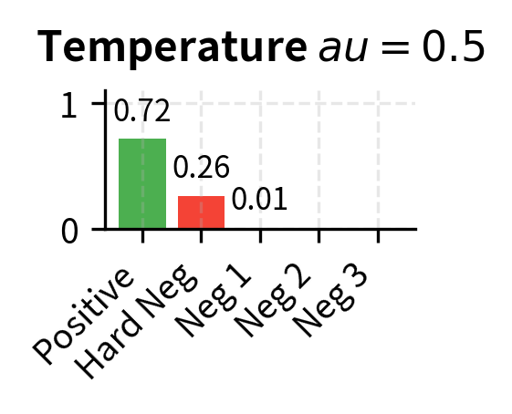
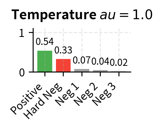
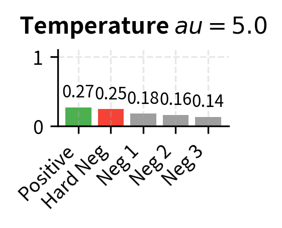
The temperature parameter controls the sharpness of the softmax distribution, and understanding its role is essential for building good intuition about contrastive training dynamics. A small (e.g., 0.05) makes the distribution peaky, amplifying differences between scores and forcing the model to be very confident about which candidate is the positive. A larger (e.g., 1.0) produces a flatter distribution, making the task easier but potentially learning less discriminative representations. This is the same temperature concept we saw in Part XVIII when discussing decoding temperature for text generation, but applied here during training rather than inference.
Let's build intuition for why matters by tracing through a concrete numerical example. With , similarity scores pass through the softmax relatively unchanged. A score of 0.7 for the positive and 0.6 for a negative yields a modest difference after exponentiation: versus . But with , those same scores become versus . A score difference of 0.1 between the positive and the best negative gets amplified by a factor of 20 before the softmax, which transforms what was a gentle preference into an overwhelming one. This forces the model to create larger gaps between positive and negative scores, producing more discriminative embeddings. The tradeoff is that very small temperatures can make training unstable, because the gradients become extremely sensitive to small changes in similarity scores. In practice, the temperature is often treated as a hyperparameter to be tuned, and some models even learn it during training.
Why InfoNCE Dominates
The InfoNCE loss has become the standard for contrastive retrieval training for several interconnected reasons, each of which illuminates a different aspect of what makes a good training objective:
- Richer gradient signal: Each training example provides information about how the query relates to all candidates simultaneously, not just one negative. With the triplet loss, a single training step only says "be closer to the positive than to this one negative." With InfoNCE, a single training step says "be closer to the positive than to all of these negatives," and the softmax probability distribution encodes the relative difficulty of each negative. Negatives that the model already handles well contribute little to the gradient, while negatives that the model confuses with the positive contribute heavily. This natural weighting of the gradient is far more efficient than the all-or-nothing signal of the triplet loss.
- Natural probabilistic interpretation: The loss directly models , making it a proper scoring function. This means the learned similarity scores have a meaningful interpretation: they are proportional to the log-probability that a passage is relevant to the query, given a set of alternatives. This probabilistic grounding connects the training objective to the downstream task of ranking, where you want the highest-scoring passage to be the most relevant one.
- Scales with negatives: As we increase , the task becomes harder and the learned representations become more discriminative. Research consistently shows that more negatives lead to better retrieval quality, up to a point. This scaling property is unique to the multi-class formulation; the triplet loss, by contrast, does not naturally benefit from having more negatives because it processes them one at a time.
The connection between number of negatives and representation quality is not coincidental; it reflects a deep theoretical property of the InfoNCE objective. Information-theoretically, InfoNCE provides a tighter lower bound on the mutual information between queries and relevant passages as grows. More negatives mean the model must learn finer distinctions, which directly translates to better retrieval. Intuitively, if you have to pick the correct passage from among 5 candidates, you can get away with coarse features. But if you must pick the correct passage from among 500 candidates, many of which are topically similar, you need representations that capture subtle semantic differences. The InfoNCE objective with large naturally induces this pressure.
In-Batch Negatives
Training with InfoNCE naturally raises a question: where do the negatives come from? The naive approach is to sample random passages from the corpus for each query. But this requires encoding extra passages per training step, which is computationally expensive, since each passage must flow through a full BERT encoder to produce its embedding. If you want 127 negatives per query and your batch has 128 queries, the naive approach requires encoding additional passages per step. In-batch negatives provide an elegant solution that eliminates this overhead entirely.
The Core Idea
The insight behind in-batch negatives comes from recognizing a simple but powerful fact about mini-batch training. Consider a mini-batch of query-positive pairs: . For query , its positive passage is . But the positive passages of all other queries in the batch, , are almost certainly irrelevant to . A passage about Shakespeare is unlikely to be relevant to a query about photosynthesis, even though both happen to be in the same mini-batch. So we can reuse them as negatives, extracting additional training signal from data we have already encoded.
This is the in-batch negatives trick: each query in a batch of size automatically gets negatives without encoding a single additional passage. The computational cost is essentially zero beyond what you would already pay for a standard forward pass, because all the passage embeddings are computed as part of the normal training step. The similarity computation for the entire batch can be expressed as a single matrix multiplication:
where:
- : the similarity matrix where entry is the similarity between query and passage
- : the matrix of query embeddings ( is batch size, is embedding dimension)
- : the matrix of passage embeddings
- : the transpose operation
This single matrix multiplication produces all pairwise similarity scores at once, exploiting the massive parallelism of modern GPUs. The structure of the resulting matrix is elegant and informative. The diagonal entries are the positive scores, capturing the similarity between each query and its own matched passage . The off-diagonal entries where are the negative scores, representing the similarity between query and the passage that belongs to some other query . This means the labels for the cross-entropy loss are simply the indices : query 0 should match passage 0, query 1 should match passage 1, and so on. The entire loss computation reduces to a standard cross-entropy call with these diagonal labels.
The similarity matrix makes the structure clear: each row corresponds to a query's similarity against all passages in the batch. The diagonal contains the positive scores (query with passage ), and every off-diagonal element is a negative. With random initialization, all scores are small and roughly similar, reflecting the fact that the encoders have not yet learned any meaningful structure. The InfoNCE loss for the entire batch is simply cross-entropy with the diagonal as the target:
With random initialization, the similarity scores are small and roughly equal, resulting in a uniform probability distribution (approximately 0.25 for each passage). The model has not yet learned to assign higher probability to the positive passage. This is exactly what we expect: before contrastive training, the embeddings carry no information about query-passage relevance, so every candidate looks equally plausible. Training will break this symmetry, pushing the probability mass toward the correct positive.
Why Batch Size Matters Enormously
With in-batch negatives, the number of negatives equals . This creates a direct and consequential link between batch size and training quality. A batch size of 32 gives 31 negatives per query, while a batch size of 512 gives 511 negatives. The difference is not merely quantitative; it is qualitative. With 31 negatives, the -way classification task is relatively easy, and the model can achieve a low loss without learning particularly fine-grained representations. With 511 negatives, the model must correctly identify the positive among hundreds of alternatives, many of which may be somewhat topically related by chance. Research on DPR and similar models consistently shows that larger batch sizes produce substantially better retrieval models, with gains that are especially pronounced when moving from small batches (16 or 32) to medium batches (128 or 256).
However, there's a practical tension. Larger batches require more GPU memory because you must simultaneously hold all query and passage embeddings and compute the similarity matrix. For with embeddings in 32-bit floating point, the embeddings alone require about 0.75 MB, which is modest. But the BERT forward and backward passes for 128 queries and 128 passages are far more memory-intensive, often requiring multiple gigabytes of GPU RAM. This is one reason why contrastive retrieval training often uses multi-GPU setups with techniques like gradient accumulation or cross-GPU negative sharing, where negatives are gathered from all GPUs to create effectively larger batches without requiring a single GPU to hold everything. For example, with 8 GPUs each processing 16 examples, cross-GPU sharing yields in-batch negatives per query, matching the effective batch size of 128 without any single GPU needing to encode more than 16 queries and 16 passages.
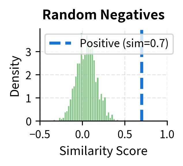
The Random Negative Problem
In-batch negatives are efficient but have a flaw: they're essentially random negatives. Because the queries in a mini-batch are drawn from the dataset without regard to topical similarity, the passages associated with other queries are, in most cases, completely unrelated to any given query. In a large corpus, a randomly selected passage is overwhelmingly likely to be completely irrelevant to a query. This makes the contrastive task too easy. The model quickly learns to distinguish obviously irrelevant passages (e.g., a passage about cooking when the query is about quantum physics) but struggles with subtle distinctions (e.g., two passages about quantum entanglement where only one actually answers the question).
To understand why easy negatives are wasteful, consider what happens to the loss and its gradients. When a negative passage is obviously irrelevant, its similarity score with the query is already much lower than the positive's score. After exponentiation in the softmax, such a negative contributes almost nothing to the denominator, and therefore almost nothing to the gradient. The model receives virtually no learning signal from this example. It is analogous to giving a student a multiple-choice exam where the wrong answers are absurdly implausible: they will get every question right without learning anything about the subject.
This is analogous to a problem we saw in Part IV with negative sampling for Word2Vec: randomly sampled negatives are useful for initial training but don't push the model to learn fine-grained distinctions. The solution there was the same as the solution here: we need harder negatives.
Hard Negative Mining
Hard negatives are passages that are superficially similar to the query or the positive passage but are not actually relevant. They force the model to learn beyond surface-level matching and develop a deeper understanding of what makes a passage truly relevant to a query. If in-batch negatives teach the model to distinguish apples from oranges, hard negatives teach it to distinguish a Granny Smith from a Honeycrisp, both of which are apples but differ in ways that matter.
What Makes a Negative "Hard"?
Negatives fall on a spectrum from trivial to hard, and the position of a negative on this spectrum determines how much the model can learn from it:
- Trivial negatives: Completely unrelated passages. "What is photosynthesis?" paired with a passage about medieval architecture. The model separates these easily after minimal training, because the vocabulary, topic, and semantic content are entirely different. These examples contribute negligible gradients.
- Medium negatives: Topically related but non-answering passages. "What is photosynthesis?" paired with a passage about chloroplasts that doesn't actually explain the process. These share vocabulary and topic but differ in specificity. The model must learn that topical overlap is necessary but not sufficient for relevance.
- Hard negatives: Passages that seem highly relevant but don't answer the query. "What is photosynthesis?" paired with a passage that defines cellular respiration using similar terminology (e.g., mentioning "energy conversion in plant cells"). These require genuine semantic understanding to distinguish, because the surface-level features of vocabulary, sentence structure, and topic all point toward relevance, yet the passage fails to provide the information the query actually seeks.
The key insight is that training on mostly trivial negatives wastes gradient updates. The loss is already near zero for these examples, so the model learns nothing from them. Hard negatives, by contrast, produce meaningful gradients that push the model to learn the fine-grained distinctions that matter for retrieval quality. They are the examples that sit near the decision boundary between "relevant" and "irrelevant" in the embedding space, and it is precisely at this boundary that the model's representations need the most refinement.
Sources of Hard Negatives
There are several practical approaches to finding hard negatives, each exploiting a different notion of "surface similarity" to identify passages that will challenge the model:
BM25 negatives. Use BM25 (which we covered in Part II) to retrieve the top- passages for each query, then exclude the known positives. BM25 finds passages with high lexical overlap, which are topically related but often not the right answer. These form excellent hard negatives because they have exactly the surface-level features a naive model might rely on: shared keywords, matching entities, and overlapping phrases. By training the model to distinguish these BM25-retrieved passages from the true positive, you force it to learn that lexical overlap alone does not constitute semantic relevance, pushing it toward a deeper understanding of meaning.
Model-based negatives. Use the retrieval model itself (or a previous checkpoint) to find its highest-scoring non-relevant passages. These are the passages the model currently "thinks" are relevant but actually aren't, precisely the errors the model most needs to learn from. This creates an iterative training loop: train the model, use it to mine hard negatives, retrain on those negatives, and repeat. Each iteration produces harder negatives than the last, because the model has corrected its previous mistakes and the remaining errors are increasingly subtle. This approach is sometimes called "self-mining" or "iterative hard negative mining," and it can yield significant improvements over static negative sets, though it comes with the computational cost of periodically re-encoding the corpus.
Cross-query negatives. The positive passage for a closely related query can serve as a hard negative. If query is "When was the Eiffel Tower built?" and is "Who designed the Eiffel Tower?", the positive passage for might discuss Gustave Eiffel's design process without mentioning the construction year, making it a hard negative for . These negatives are particularly valuable because they are relevant to the topic but address a different information need, forcing the model to distinguish between queries that share a subject but differ in intent.
Gold negatives from annotations. Some datasets include explicit negative annotations where annotators mark passages as "related but not relevant." These are the highest-quality hard negatives but the most expensive to obtain, because they require human judgment to identify passages that are deceptively similar to the true positive. When available, they provide the clearest training signal, as there is no risk of mislabeling.
The Hard Negative Balancing Act
Using only hard negatives can actually hurt training, a counterintuitive finding that reveals an important subtlety of the contrastive learning framework. If every negative is nearly indistinguishable from the positive, the loss landscape becomes very noisy and the model may struggle to converge. The gradients from each training step will be large and highly variable, pushing the model in inconsistent directions. Worse, some mined hard negatives may actually be false negatives, passages that truly are relevant but aren't labeled as such. Training the model to push these away degrades performance, because the model is being rewarded for making incorrect predictions.
The false negative problem is especially acute with model-based mining. If the current model assigns a high score to a passage, and that passage is excluded from the positive set simply because it wasn't in the original annotations, there is a real chance the passage is genuinely relevant. Pushing it away not only wastes a gradient step but actively corrupts the learned representation. This is why some recent work explores techniques for detecting and mitigating false negatives, such as denoising heuristics or soft labels that give partial credit to borderline passages.
The best practice is to mix hard negatives with random (in-batch) negatives. DPR, for example, uses one BM25 hard negative per query combined with in-batch negatives from the rest of the batch. This gives the model a mix of easy examples (for stable gradients and smooth convergence) and challenging examples (for learning fine distinctions and pushing the decision boundary). The easy negatives provide a reliable "floor" of gradient signal that keeps the model moving in the right direction, while the hard negatives provide the "ceiling" of information that drives the model toward high-quality representations.
Let's visualize how different negative strategies affect the difficulty of the contrastive task:
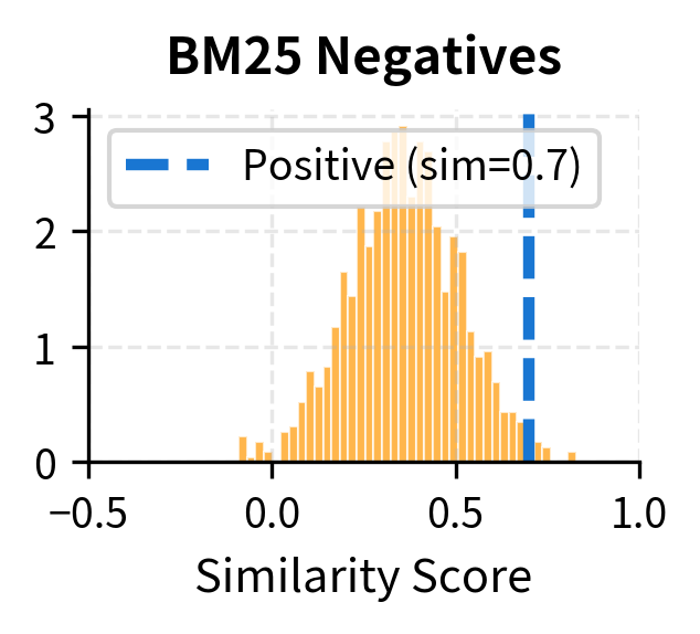
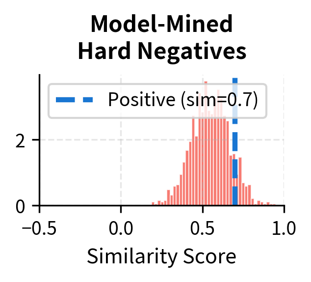
The visualization makes the point clear. With random negatives, the positive score is far from the negative distribution, so the model can trivially distinguish them: the positive sits comfortably to the right of essentially all negatives, and the softmax assigns it a high probability without the model needing to learn anything subtle. With BM25 negatives, there's more overlap, requiring the model to work harder, because some negatives have similarity scores that approach the positive's score, and the model must push these down while keeping the positive high. With model-mined hard negatives, the negative distribution pushes right up against the positive score, demanding the model learn very precise distinctions. In this regime, even small improvements in the model's ability to separate positives from confusing negatives translate directly into better retrieval quality.
DPR Training Procedure
Dense Passage Retrieval (DPR), introduced by Karpukhin et al. in 2020, was one of the first systems to demonstrate that a contrastive-trained dense retriever could outperform BM25 on open-domain question answering. Its training procedure combines the techniques we've discussed into a coherent pipeline and serves as the template for most subsequent dense retrieval models. By examining DPR in detail, we can see how the abstract ideas of contrastive loss, in-batch negatives, and hard negative mining come together into a working system.
Architecture
DPR uses a dual-encoder architecture with two independent BERT-base models (as we covered in Part XVII): one for queries and one for passages. Each encoder takes its input text, processes it through 12 transformer layers, and produces a -dimensional embedding by taking the [CLS] token representation from the final layer. This [CLS] embedding serves as a single fixed-size summary of the entire input sequence, compressing all the information in a query or passage into a vector that can be compared via simple arithmetic.
The choice to use separate encoders for queries and passages is deliberate and reflects the asymmetric nature of the retrieval task. Queries are typically short (5-15 tokens) while passages are longer (up to 256 tokens), and their linguistic properties differ substantially. A query is often a question or a fragmentary phrase, while a passage is a coherent piece of expository text. Separate encoders allow each to specialize: the query encoder can learn to interpret the intent behind terse questions, while the passage encoder can learn to extract the key information from longer prose. However, both encoders share the same architecture (BERT-base), just initialized from the same pretrained checkpoint and then fine-tuned independently through the contrastive training process.
The similarity function is a simple dot product:
where:
- : the similarity score used by DPR
- : the embedding output of the query encoder
- : the embedding output of the passage encoder
- : the transpose operation, computing the dot product between the two vectors
No learned projection layers, no cosine similarity normalization. The dot product is chosen for its computational simplicity at retrieval time: computing a dot product between two 768-dimensional vectors requires only 768 multiplications and 767 additions, making it fast enough to score millions of candidates per second with appropriate indexing. This efficiency is essential because at inference time, the retriever must search over the entire corpus, which may contain millions of passages, to find the top- most relevant results. We'll explore the indexing techniques that make this feasible in the chapters on vector similarity search and indexing.
Training Data
DPR was trained on five question-answering datasets: Natural Questions, TriviaQA, WebQuestions, CuratedTREC, and SQuAD. For each question, the positive passage is the paragraph containing the answer. The training set contains roughly 60,000 question-passage pairs. This is a relatively modest dataset by modern standards, but the contrastive training framework with in-batch negatives extracts a surprisingly large amount of training signal from each example, because every passage in the batch serves as a negative for every other query.
The negative passages for each question come from three sources, combined into a single training example:
- In-batch negatives: The positive passages from all other questions in the mini-batch ( negatives). These provide a large, diverse set of mostly easy negatives that give the softmax distribution its broad shape.
- One BM25 hard negative: The highest-scoring BM25 passage that doesn't contain the answer string. This provides a lexically similar but non-answering passage, forcing the model to learn that keyword overlap does not equal relevance.
- One gold negative (when available): A passage annotated by humans as relevant-looking but incorrect. These are the highest-quality negatives in the training set, providing a clear signal about exactly the kind of mistake the model should avoid.
This mixture is carefully chosen, and the DPR paper includes ablation studies showing that each component contributes to the final performance. The in-batch negatives provide a large number of diverse (mostly easy) negatives for a rich softmax distribution, ensuring that the gradients are stable and well-behaved. The BM25 hard negative adds one challenging example that forces the model beyond lexical matching, directly addressing the failure mode of relying on surface features. The combination proved more effective than using any single negative strategy alone, confirming the principle that a diverse mix of negative difficulties produces the best training dynamics.
The Loss Function
The DPR loss is a direct application of InfoNCE. For a batch of questions, with each question having one positive passage, one BM25 hard negative, and in-batch negatives, the loss for question is:
where:
- : the loss for the -th query in the batch
- : similarity with the true positive passage
- : similarity with the BM25 hard negative
- : sum of exponentials of similarities with in-batch negatives (positives from other queries)
- : the exponential function ensuring positive values
- : the negative log-likelihood maximizing the probability of the positive pair
To understand this formula concretely, consider what the denominator contains. There are three groups of terms. The first term, , is the positive passage's contribution. The second term, , is the BM25 hard negative's contribution, representing the single most challenging distractor. The remaining terms in the summation, , are the contributions from all other passages in the batch. The model must push the numerator (the positive) to dominate this entire denominator, which means simultaneously pushing the positive score up and all negative scores down.
Note that DPR uses (no temperature scaling). The temperature is effectively absorbed into the magnitude of the learned embeddings: since there is no normalization step, the model is free to learn embeddings of whatever magnitude is needed to produce well-calibrated softmax distributions. The total batch loss averages over all questions, so each training step updates the encoders based on the collective signal from every query-passage interaction in the batch.
Training Hyperparameters
The specific training configuration that DPR found effective includes:
- Batch size: 128 (using 8 GPUs with 16 examples per GPU, sharing negatives across GPUs to get the full 127 in-batch negatives).
- Learning rate: with linear warmup and linear decay.
- Epochs: 40 epochs over the training data.
- Sequence lengths: 256 tokens for passages, 32 tokens for queries.
- Optimizer: Adam, consistent with standard BERT fine-tuning practices we discussed in Part XXIV.
The large batch size is critical and deserves special emphasis. The DPR paper's ablation studies showed that increasing batch size from 16 to 128 improved top-20 retrieval accuracy by over 3 percentage points, directly demonstrating the importance of having many in-batch negatives. This improvement is not just a marginal gain; it represents the difference between a system that is competitive with BM25 and one that clearly surpasses it. The choice of 128 was not arbitrary but reflected the largest batch size achievable on the available hardware (8 V100 GPUs), and subsequent work has shown that even larger batch sizes can yield further improvements when the compute budget allows.
Code Implementation
Let's implement a simplified version of DPR training to make these concepts concrete. We'll use the transformers library for the encoder and build the contrastive training loop step by step.
Setting Up the Encoders
First, let's set up the dual encoder architecture using a pretrained model:
Each encoder extracts the [CLS] token representation from BERT's final layer, producing a 768-dimensional vector. As we discussed in Part XVII, the [CLS] token is designed to aggregate sequence-level information during pretraining. At initialization, both encoders start from the same pretrained BERT weights, but because they are separate nn.Module instances, they will diverge during fine-tuning as the contrastive loss pushes each one to specialize for its respective input type: short queries versus longer passages.
Building the Contrastive Loss
Now let's implement the InfoNCE loss with in-batch negatives and an optional hard negative. The implementation follows the mathematical formulation closely, constructing the score matrix and then delegating the softmax and negative log-likelihood computation to PyTorch's built-in cross_entropy function:
The key insight in this implementation is how the labels work and how the score matrix is structured. For query , the correct positive passage is at index in the score vector, because it corresponds to the diagonal of the in-batch similarity matrix. The hard negative, if present, is appended as an additional column at index , so the score tensor for each query has shape : the first entries are the in-batch similarities (one of which is the positive), and the last entry is the hard negative. The cross_entropy function computes the softmax over this entire vector and applies the negative log-likelihood to the position indicated by the label, which is always the diagonal index . This single function call handles the entire InfoNCE computation, including the numerator, denominator, exponentiation, normalization, and log, in a numerically stable way.
Demonstrating the Training Step
Let's create a small example to see the loss in action. We define four query-passage-negative triplets that illustrate the kind of data a real DPR training pipeline would process:
Notice how each hard negative is topically related to its query but does not actually answer the question. The first hard negative mentions France but says nothing about its capital. The second mentions Shakespeare but does not attribute Romeo and Juliet to him. These are exactly the kind of BM25-style hard negatives that DPR uses: high lexical overlap, low semantic relevance to the specific information need.
The output confirms that the encoder produces 768-dimensional vectors for all inputs, matching the hidden size of the BERT-base model. Each query, positive passage, and hard negative has been compressed into a single point in this 768-dimensional space. Before training, these points are placed essentially at random with respect to the relevance relationships we care about.
Now let's compute the similarity matrix and loss to see how the untrained model performs:
Before contrastive training, the similarity scores are essentially random. The diagonal (positive pairs) doesn't stand out from the off-diagonal (negatives). This is the expected baseline: the pretrained BERT encoders produce embeddings that capture general linguistic features, but they have received no signal about which query-passage pairs should be considered relevant. The contrastive training process will reshape this embedding space so that the diagonal entries (true positives) consistently dominate their respective rows. Let's see the loss:
The loss is close to the random baseline ( for a uniform distribution over candidates), confirming that the untrained model can't distinguish positives from negatives. The random baseline represents the loss you would get if the model assigned equal probability to every candidate, which is exactly what happens when similarity scores are uniform. For four candidates, ; for five candidates (with the hard negative), . Any deviation from these values before training reflects minor random asymmetries in the pretrained embeddings rather than any genuine retrieval ability.
Training Loop
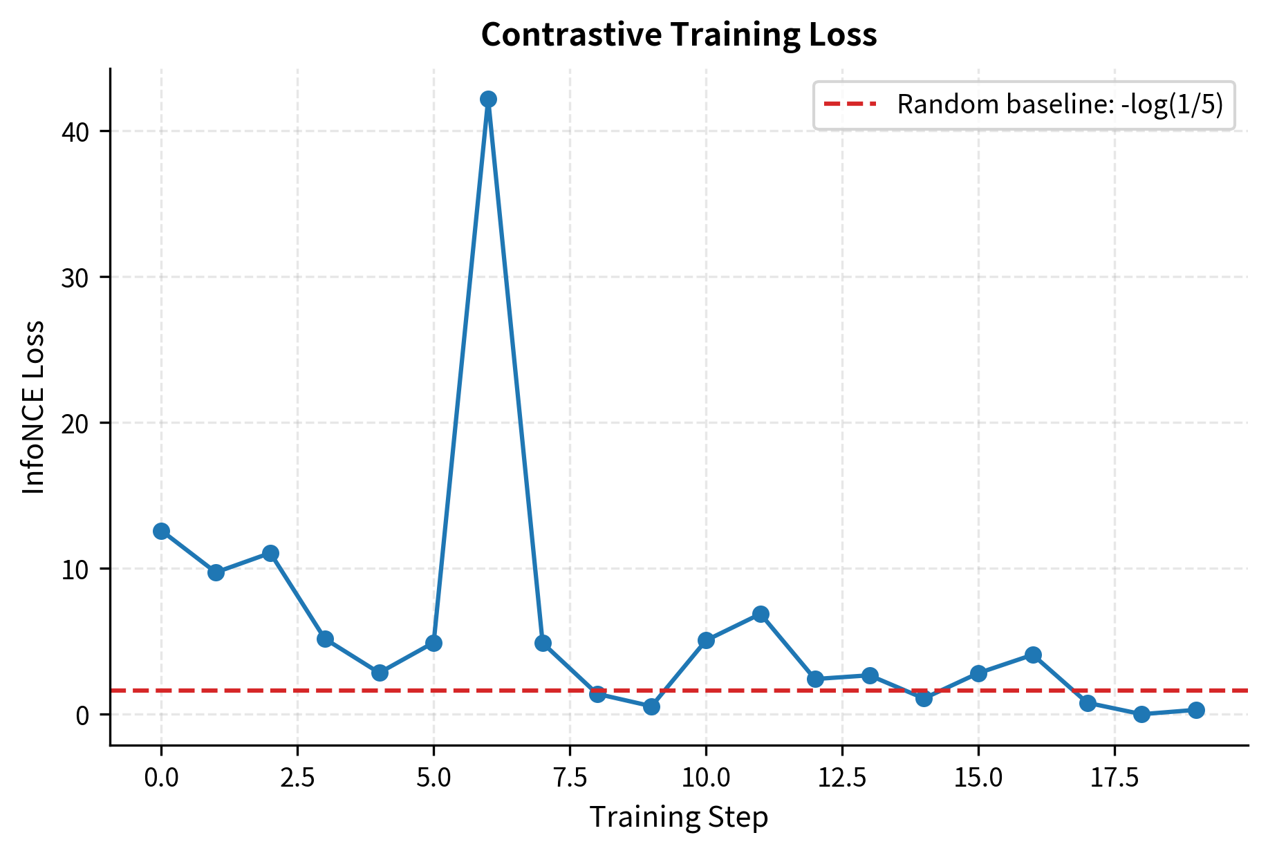
Let's run a few training steps to show the loss decreasing:
Let's examine the similarity matrix after training to see if the model has learned to differentiate positives from negatives:
Even with just 20 steps on 4 examples (far less than real training), you can see the model beginning to push diagonal scores higher than off-diagonal ones. In a production DPR training run with 60,000 examples over 40 epochs and batch sizes of 128, the model would fully converge, producing a similarity matrix where the diagonal entries clearly dominate every row.
Simulating Hard Negative Mining
Let's demonstrate the BM25 hard negative mining process that DPR uses. We'll simulate it with a simple TF-IDF retriever, which shares BM25's core mechanism of favoring passages with high lexical overlap with the query:
Notice how the mined hard negatives are topically relevant to each query but don't actually answer the question. For the query about France's capital, the retriever surfaces passages that mention France or Paris but in a different context. For the Shakespeare query, it finds passages about Shakespeare that discuss other works rather than Romeo and Juliet. This is exactly the property that makes them valuable for training: they force the model to go beyond keyword matching and learn to distinguish between passages that share surface features with the true answer and passages that actually contain the information being sought.
Key Parameters
The key parameters for Dense Passage Retrieval training are:
- temperature: Scales the similarity scores before softmax. DPR uses 1.0 (no scaling).
- batch_size: Number of queries per batch. Critical for in-batch negatives; larger batches (e.g., 128) improve performance.
- learning_rate: Step size for the optimizer. Common values are around .
- weight_decay: Regularization parameter to prevent overfitting.
- max_length: Maximum token sequence length. Queries and passages often have different limits (e.g., 32 and 128).
Training Dynamics and Considerations
Beyond the basic setup, several nuances in contrastive training significantly impact the final model quality. These considerations arise from the interaction between the loss function's mathematical properties and the practical realities of training large models on limited hardware.
Symmetric vs. Asymmetric Loss
The loss we've described is asymmetric: for each query, we find its positive among all passages. In other words, we compute a row-wise softmax over the similarity matrix, asking each query to select its correct passage from the columns. You can also add a symmetric term where, for each passage, you find its matching query among all queries. This corresponds to a column-wise softmax, asking each passage to select the query it belongs to from the rows:
where:
- : the bidirectional contrastive loss
- : the standard InfoNCE loss computed row-wise (queries selecting passages)
- : the InfoNCE loss computed column-wise (passages selecting queries)
The symmetric formulation provides additional training signal by exploiting the same similarity matrix from both directions. In the asymmetric case, the passage encoder only receives gradients based on how passages are scored by queries. In the symmetric case, the passage encoder also receives gradients from the task of selecting the correct query, which can help it learn more robust representations. Symmetric loss is used by models like CLIP and some sentence embedding models. DPR uses only the asymmetric query-to-passage direction, which is a natural choice for retrieval since the operational task is always "given a query, find the passage" rather than the reverse.
Gradient Caching for Large Batches
As we noted, larger batches produce better models because they provide more in-batch negatives. But large batches hit GPU memory limits quickly since each BERT encoder's forward and backward passes consume substantial memory, often several gigabytes for a batch of 128 sequences through a BERT-base model. Gradient caching (sometimes called GradCache) addresses this by decoupling the batch size used for contrastive comparison from the batch size used for the encoder forward pass. The procedure works in four stages:
- Compute all embeddings in small chunks (with
torch.no_grad()to save memory). For example, process 16 queries at a time rather than all 128, caching the resulting embeddings. - Compute the full similarity matrix and loss using the cached embeddings. Since the embeddings are just vectors, the matrix multiplication is cheap even for large .
- Backpropagate through the loss to get gradients on embeddings. This tells us how each embedding should change to reduce the loss.
- Re-run the encoder forward passes in small chunks, using the embedding gradients to compute parameter gradients via the chain rule.
This technique decouples the batch size for contrastive learning from the batch size that fits in GPU memory during the encoder forward pass. You can use a contrastive batch size of 4096 while only ever processing 32 sequences through the encoder at a time, achieving the representational benefits of massive in-batch negative sets without exceeding your GPU's memory capacity.
Asynchronous Index Refresh
In iterative hard negative mining, you periodically re-encode the entire corpus to find new hard negatives using the updated model. This is expensive: for a corpus of 21 million passages (as in DPR's Wikipedia corpus), re-encoding takes hours even on multiple GPUs, because every passage must flow through the passage encoder to produce a fresh embedding that reflects the model's current parameters. A practical approach is asynchronous refresh, where you mine hard negatives using a slightly stale model checkpoint while training continues with the current model. The mined negatives are based on the model as it was several training steps ago, which means they may not perfectly reflect the current model's failure modes. The staleness introduces some noise, but the efficiency gain is worth it, and empirical results show that even moderately stale negatives provide substantial benefit over using no hard negative mining at all. More sophisticated systems use a rolling refresh schedule, re-encoding a fraction of the corpus each step so that the index is always partially fresh without ever requiring a full re-encoding pause.
Limitations and Impact
Contrastive learning for retrieval represented a watershed moment in information retrieval, proving that learned dense representations could match or exceed decades of tuned sparse methods like BM25. But the approach has important limitations that continue to drive research.
The most fundamental limitation is the dependence on negative quality and quantity. As we've seen, too-easy negatives waste training signal, while too-hard negatives (especially false negatives) can actively hurt the model. Getting the balance right requires careful engineering, and the optimal strategy varies across domains and datasets. Additionally, the strong batch size requirements mean that high-quality contrastive training demands significant compute resources, often 8 or more GPUs to achieve the batch sizes (128 or larger) where in-batch negatives become effective. This creates a meaningful barrier for researchers and practitioners without access to large GPU clusters.
A more subtle issue is that the dual-encoder architecture, while efficient at retrieval time, is fundamentally limited by the information bottleneck of the fixed-size embedding. A single 768-dimensional vector must capture everything about a passage that any possible query might ask about. This is why even well-trained dense retrievers sometimes miss relevant passages that a cross-encoder (which directly attends across query and passage tokens) would catch. This limitation motivates the reranking stage we'll discuss later in this part, where a more expensive cross-encoder re-scores the top candidates from the initial retrieval.
Despite these limitations, the contrastive learning framework has proven remarkably versatile. The same ideas power sentence embeddings (as we'll explore in the next chapter on embedding models), image-text matching (CLIP), code search, and multilingual retrieval. The DPR training recipe, specifically the combination of in-batch negatives, BM25 hard negatives, and InfoNCE loss, has become the starting point for nearly every modern dense retrieval system.
Summary
Contrastive learning trains retrieval models by teaching them to distinguish relevant passages from irrelevant ones. The key concepts covered in this chapter are:
-
InfoNCE loss frames retrieval as multi-class classification over similarity scores. The model must assign the highest probability to the true positive passage among all candidates. A temperature parameter controls the sharpness of the softmax distribution.
-
In-batch negatives reuse the positive passages of other queries in a mini-batch as negatives, producing negatives for free from a batch of examples. This makes batch size a critical hyperparameter: larger batches provide more negatives and consistently yield better models.
-
Hard negative mining provides challenging examples that share surface features with the positive but aren't actually relevant. BM25 retrieval is the most common source, since it finds lexically similar passages that lack true semantic relevance. Mixing hard negatives with easier in-batch negatives gives the best training dynamics.
-
DPR's training procedure combines these ideas into a complete system: two BERT-base encoders (one for queries, one for passages), trained with InfoNCE loss over in-batch negatives plus one BM25 hard negative per query, at batch size 128 across 8 GPUs.
The next chapter on document chunking will address a practical prerequisite for applying these retrieval models: how to split long documents into passages that are the right size for encoding and retrieval.
Quiz
Ready to test your understanding? Take this quick quiz to reinforce what you've learned about contrastive learning for retrieval.

Comments