

Master IVF indexes for scalable vector search. Learn clustering-based partitioning, nprobe tuning, and IVF-PQ compression for billion-scale retrieval.

This article is part of the free-to-read Language AI Handbook
Choose your expertise level to adjust how many terms are explained. Beginners see more tooltips, experts see fewer to maintain reading flow. Hover over underlined terms for instant definitions.
IVF Index
In the previous chapter, we explored HNSW, a graph-based approach to approximate nearest neighbor search that builds navigable small-world graphs for fast traversal. HNSW is powerful but comes with a significant memory cost. The graph structure itself must be stored alongside the vectors, and the entire index typically needs to reside in memory. For collections of tens or hundreds of millions of vectors, this memory requirement can become prohibitive.
The Inverted File Index (IVF) takes a fundamentally different approach. Instead of building a graph, it partitions the vector space into regions using clustering, then organizes vectors by which region they belong to. At query time, rather than searching all vectors, you search only the vectors in the few regions closest to your query. This is analogous to a library organizing books by subject. If you want a book about marine biology, you don't scan every shelf; you go directly to the science section.
The core insight behind IVF is that vectors that are close in the embedding space tend to cluster together. By grouping similar vectors and only searching relevant groups, IVF dramatically reduces the number of distance computations needed. The approach is conceptually simple, scales gracefully to very large datasets, and can be combined with compression techniques like Product Quantization, which we'll cover in the next chapter, to handle billion-scale collections.
The Clustering Approach
IVF works in two phases: an offline indexing phase that partitions the vector space, and an online query phase that searches only the relevant partitions. The advantage of this two-phase design is that the expensive work of organizing the data happens once during indexing so that every subsequent query can exploit that precomputed structure to avoid scanning the full dataset. Let us examine each phase in detail, starting with how the index is built.
Index Construction
The indexing phase uses k-means clustering to divide the vector space into distinct regions, called Voronoi cells. Each cell is defined by its centroid, a representative point at the center of the cluster. The process proceeds through three steps: first we discover where the natural groupings in the data lie, then we assign every vector to its closest grouping, and finally we build the data structure that makes retrieval efficient. Here is how the process works:
- Train centroids: We begin by discovering natural groupings in the data. The fundamental question at this stage is: if we had to summarize the entire dataset using only representative points, where should those points be placed so that every vector in the collection is as close as possible to at least one of them? K-means clustering answers precisely this question. It identifies centroids that serve as representative points for different regions of the vector space.
K-means clustering finds representative points (centroids) by grouping vectors so that vectors within each group are as close as possible to their group's center. This minimizes the total "within-cluster" distance across all groups. The algorithm accomplishes this iteratively: it starts with an initial guess for where the centroids should be, then repeatedly refines those positions by reassigning vectors and recalculating centers until the arrangement stabilizes.
Formally, k-means seeks to minimize the objective function:
where:
- : the number of clusters (centroids) we want to create, controlling how finely we partition the space
- : the -th centroid, a -dimensional vector representing the center of cluster
- : the set of all vectors assigned to cluster
- : a vector in the dataset
- : the squared Euclidean distance between vector and centroid , measuring how far the vector is from its assigned centroid
- : the dimensionality of each vector in the dataset
This objective function captures the total within-cluster variance, which serves as a single number summarizing how well the centroids represent their assigned vectors. A lower value means tighter, more compact clusters where vectors are close to their centroids, exactly the property we want for IVF to work well. The inner sum accumulates distances for all vectors in cluster , measuring the spread of that individual cluster. The outer sum then combines these individual cluster costs across all clusters, yielding the total cost of the entire partitioning.
Why does the objective use squared distance rather than plain distance? The squared distance grows quadratically with separation, so vectors far from their centroid contribute disproportionately to the objective. This property encourages the algorithm to prioritize reducing large errors, naturally resulting in tight, compact clusters. A single outlier vector that is very far from its centroid will dominate the sum, pushing the algorithm to adjust the centroid positions to bring such outliers closer. The algorithm alternates between two steps: (1) assigning each vector to its nearest centroid, and (2) recomputing each centroid as the mean of all vectors assigned to it. This process repeats until the assignments stabilize (convergence). Each iteration is guaranteed to decrease (or at least not increase) the objective, which ensures that the algorithm converges, though it may settle on a local minimum rather than the global optimum.
- Assign vectors: Once centroids are established, we move to the partitioning step, where the goal is to divide the entire dataset into non-overlapping groups. Each vector is assigned to its nearest centroid, meaning the centroid to which it has the smallest Euclidean distance. This assignment is deterministic: given a fixed set of centroids, every vector maps to exactly one cluster. Formally, we assign each vector to cluster where:
where:
- : a vector in the dataset that we're assigning to a cluster based on minimum distance to centroids
- : the index of the cluster (centroid) to which is assigned
- : the operator that returns the index that minimizes the expression
- : the total number of centroids
- : the -th centroid
- : the Euclidean distance between vector and centroid
The operator finds which centroid index yields the smallest distance, making this a hard assignment: each vector belongs to exactly one cluster. This is a critical property for the IVF data structure because it means every vector appears in exactly one inverted list, avoiding duplication and keeping the index size manageable.
This assignment process creates Voronoi cells where all vectors in a cell share the same nearest centroid. Geometrically, you can think of each centroid as claiming the region of space that is closer to it than to any other centroid, and every vector falling within that region is added to that centroid's list.
- Build inverted lists: The final step of index construction is to create the data structure that makes search efficient. We build an "inverted file" where each centroid points to the list of all vectors assigned to its cell. This is the structure that query processing will use: given a centroid, we can immediately look up every vector that belongs to its cell without scanning the entire dataset.
The term "inverted file" comes from the same concept behind inverted indexes in information retrieval, which we encountered in Part II when discussing TF-IDF. In a text inverted index, each term points to its list of documents; here, each centroid points to its list of vectors. The analogy is precise: just as a text search engine uses a term to quickly locate all documents containing that term, an IVF index uses a centroid to quickly locate all vectors belonging to that region of space.
A Voronoi cell (or Voronoi region) is the set of all points in space that are closer to a particular centroid than to any other centroid. The collection of all Voronoi cells partitions the entire space with no gaps or overlaps. Every point belongs to exactly one cell.
With the index structure in place, the question naturally arises: how many centroids should we use? The number of centroids is a critical hyperparameter that balances cell granularity against centroid comparison cost. Too few centroids means each cell is large and expensive to scan; too many centroids means the coarse comparison step itself becomes a bottleneck. A common rule of thumb is to set:
where:
- : the number of centroids (clusters) in the IVF index
- : the total number of vectors in the dataset
- : the square root of , serving as a baseline for centroid count
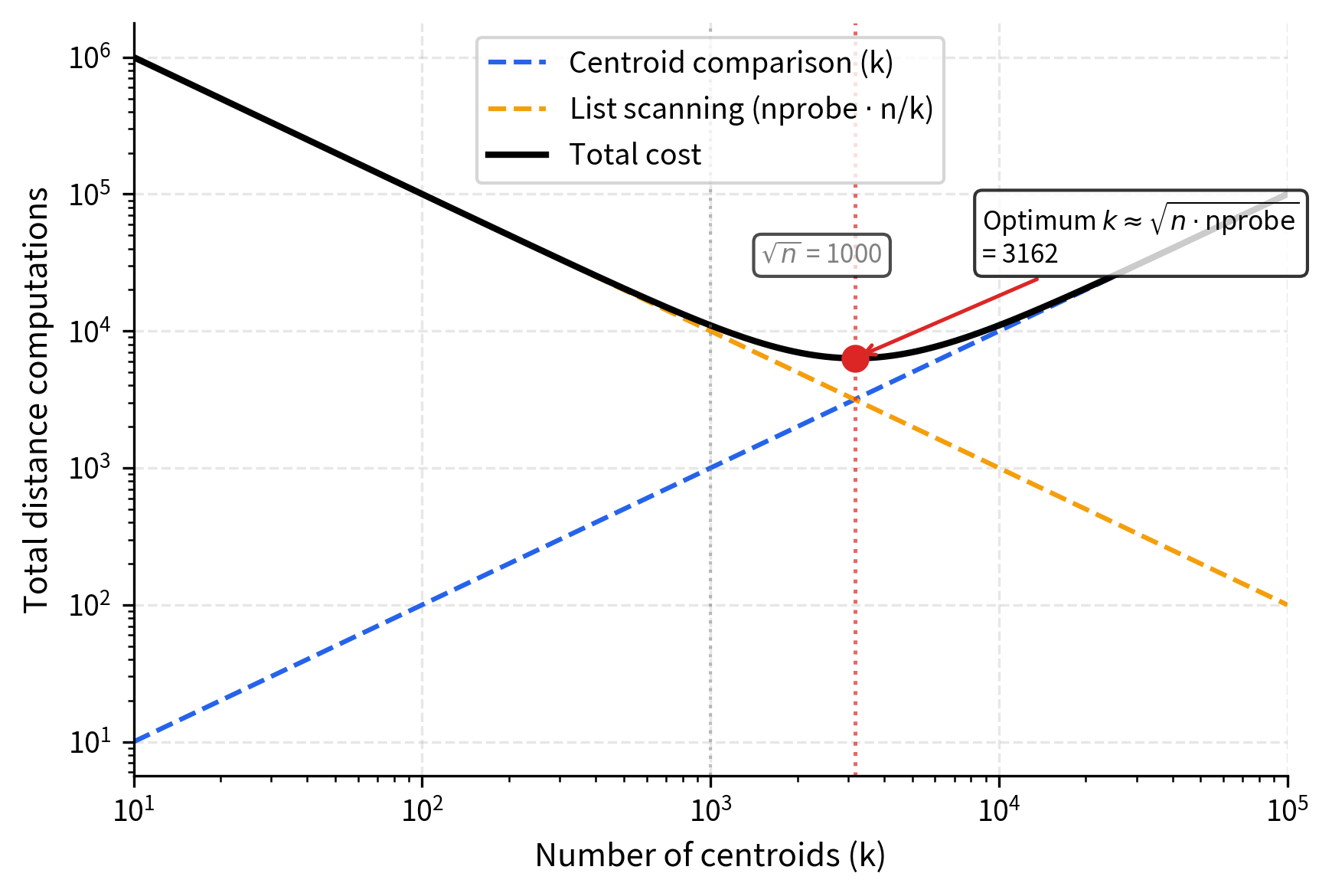
This square root relationship balances two competing costs: the cost of comparing the query to all centroids (grows with ), and the cost of scanning vectors within cells (decreases as increases because each cell becomes smaller). The square root provides a reasonable middle ground. To see why, consider that the total work is proportional to . Minimizing this expression with respect to (taking the derivative and setting it to zero) yields , which is exactly the balancing point where the two costs are equal.
In practice, values between and are commonly used.
The square root relationship emerges from balancing two costs: too few centroids means large cells (expensive to scan), while too many centroids means expensive centroid comparison. For a collection of 1 million vectors, this means roughly 1,000 to 4,000 centroids. Each centroid's inverted list then contains on average vectors. This average list size is an important quantity because it determines how much work each probe requires during the query phase.
Query Processing
With the index built and all vectors neatly organized into their respective inverted lists, we can now turn to the question of how search actually works. The key idea is to exploit the structure we built during indexing: instead of comparing the query against every vector in the dataset, we first identify which regions of space are most promising, and then restrict our search to only those regions. This transforms an exhaustive scan into a targeted one. When a query vector arrives, IVF performs these steps:
- Find nearest centroids: The first step is coarse filtering, where we identify which regions of space are worth examining in detail. We compute the distance from to all centroids which is the closest ones. This step is fast because ; we only need to perform distance computations rather than .
The intuition behind this step is straightforward. If a vector is close to the query, its centroid is likely also close to the query. Centroids represent the center of mass of their respective clusters, so the nearest centroid to the query is a strong indicator of where the nearest vectors reside. By comparing only to centroids first, we quickly narrow down which regions of space are worth examining in detail. Formally, we compute the distance from the query to each centroid:
where:
- : the query vector for which we're searching for nearest neighbors
- : the -th centroid
- : the distance between the query and centroid
- : the total number of centroids (clusters) in the IVF index
- : the number of closest centroids whose cells we will search
We then select the centroids with the smallest distances, controlling the accuracy-speed tradeoff. The selected centroids define a search neighborhood around the query. We trust that these closest regions of space contain most, if not all, of the true nearest neighbors.
-
Search inverted lists: Having identified the most promising cells, we now scan all vectors in the inverted lists of those centroids. This is an exhaustive comparison within the selected cells, where every vector in the chosen lists is compared against the query. The crucial efficiency gain is that we examine only a small subset of the total dataset rather than the entire collection.
-
Return top results: From all scanned vectors, return the top- nearest neighbors based on their distances to the query. This is the fine-grained ranking step, where we take the candidate pool gathered from the selected cells and identify which candidates are truly closest to the query. We compute the distance from the query to each candidate vector:
where:
- : the query vector
- : the -th candidate vector from the scanned cells
- : the distance between the query and candidate vector
- : the number of nearest neighbors to return (note: this reuses the symbol but refers to result count, not centroid count)
This step performs the final ranking among the candidates that survived the coarse filtering stage, selecting the truly closest vectors from the subset we examined.
We then sort all candidates by distance and select the vectors with the smallest distances as our final results. This two-stage approach, coarse filtering followed by fine-grained ranking, is what gives IVF its efficiency: the expensive exact distance computations are restricted to a small, carefully chosen subset of vectors.
Let us now quantify the cost of each step to understand where the computational savings come from. The first step requires only distance computations (comparing the query to each centroid), which is fast since the number of centroids is much smaller than the number of vectors (written as ). For a dataset of one million vectors with one thousand centroids, this coarse step examines just 0.1% of the data.
The second step searches approximately vectors. Each cell contains on average vectors (assuming balanced clustering), so searching cells means examining:
where:
- : the number of cells we search
- : the total number of vectors in the dataset
- : the number of centroids (clusters)
- : the average number of vectors per cell, assuming balanced clustering
This is typically a small fraction of the total dataset because in practice. To express this more concretely, the fraction of the total dataset that we examine is simply:
where:
- : the number of cells searched
- : the total number of centroids (cells) in the IVF index
This fraction directly controls the speedup versus brute-force search: smaller fractions mean faster queries but potentially lower recall. The relationship is intuitive: if we search half the cells, we examine roughly half the data and get roughly half the speedup.
For example, with 100 centroids and nprobe=10, we examine only about 10% of the data.
This gives us an approximate search because the true nearest neighbor might reside in a cell whose centroid was not among the closest to the query. Vectors near the boundaries between cells are the most vulnerable to being missed, because their centroid may not be the closest centroid to the query even though the vectors themselves are very close. Increasing reduces this risk at the cost of searching more vectors. This boundary effect is the fundamental source of approximation error in IVF, and understanding it is essential for choosing good parameter values.
Probe Count: The Accuracy-Speed Tradeoff
The parameter is the primary knob for controlling the tradeoff between search accuracy (recall) and search speed. To build clear intuition for how this parameter works, it helps to consider the two extreme settings and then reason about what happens in between.
When , you search only the single closest cell. This is the fastest setting but also the least accurate because any nearest neighbor that happens to sit in an adjacent cell will be missed. When (all cells), you search every vector in the dataset, which is equivalent to brute-force search with perfect recall but no speed benefit.
where:
- : the number of cells (clusters) searched at query time, ranging from 1 (fastest, least accurate) to (slowest, perfect accuracy)
- : the total number of centroids (cells) in the IVF index
These extremes illustrate the fundamental tradeoff: interpolates between a single-cell approximation and exhaustive search. Every value in between represents a different point on the accuracy-speed curve, and using IVF well means finding the right balance for your application.
In practice, you typically want values that give you high recall (say, 90-99%) while searching only a small fraction of the data. The sweet spot depends on several factors:
- How well the data clusters: If the data forms tight, well-separated clusters, even can achieve high recall. If the data is uniformly distributed with no natural clusters, you need more probes.
- The number of centroids: More centroids means smaller cells, which means more probes are needed for the same recall level. But more centroids also means each cell is smaller, so each probe is cheaper.
- The dimensionality of the vectors: Higher-dimensional spaces exhibit the "curse of dimensionality," where distances become more uniform and cluster boundaries become less meaningful, generally requiring more probes.
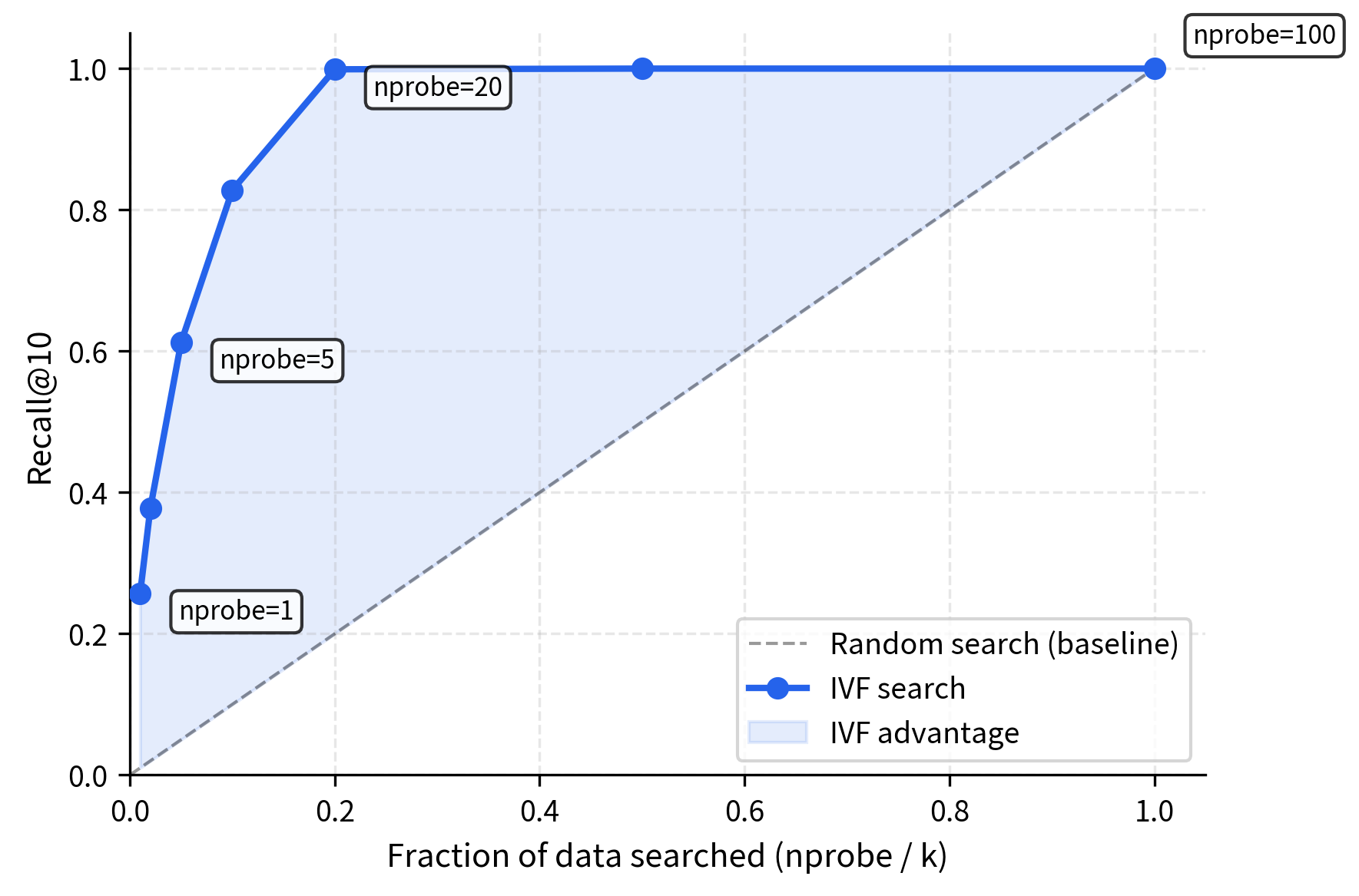
A useful mental model is to think of recall as a function of the fraction of data searched. If you have centroids and set , you search roughly:
where:
- : the number of centroids in this example
- : the number of cells we choose to search
- : the fraction of cells searched, which approximates the fraction of the dataset examined (exact if cells are perfectly balanced)
In practice, this often yields 80-95% recall depending on the dataset, because nearby cells tend to contain the true nearest neighbors. The reason recall is much higher than the fraction of data searched is precisely because IVF's clustering is not random: it groups similar vectors together, so the closest cells to the query are disproportionately likely to contain the nearest neighbors.
Analyzing the Computational Cost
Now that we understand the qualitative tradeoff, let us make it precise by analyzing the computational cost step by step. This analysis will reveal exactly where the savings come from and how the different parameters interact. For a dataset of vectors in dimensions partitioned into centroids, a query requires:
Step 1: Find nearest centroids
We compare the query vector to all centroids. Each comparison computes the distance between two -dimensional vectors. For Euclidean distance, this requires computing squared differences and summing them plus a square root (which we ignore in big-O notation). Therefore, this step costs:
where:
- : the number of centroids in the IVF index
- : the dimensionality of each vector (and each centroid)
- : the total number of operations needed to compare the query against all centroids
This cost is fixed regardless of dataset size . Whether you have one million or one billion vectors, comparing against centroids costs the same. This is one of the elegant properties of IVF: the coarse filtering step is completely independent of the number of data vectors.
Step 2: Scan inverted lists
We scan the vectors in the selected cells. Assuming roughly equal-sized cells, each cell contains approximately vectors. Thus, we scan vectors total. Each distance computation again requires operations, giving:
where:
- : the number of cells we search
- : the total number of vectors in the dataset
- : the total number of centroids (cells)
- : the average number of vectors per cell, assuming balanced clustering
- : the dimensionality of each vector
This is typically the dominant cost, since is usually much larger than . The key observation is that this cost scales linearly with . Doubling the number of probed cells exactly doubles the number of vectors we must examine, which is why query time grows linearly with as we observed in the experiments.
Total query cost
Combining both steps gives us the complete picture of what a single query costs:
where:
- : cost of comparing the query to all centroids (Step 1)
- : cost of scanning vectors in the selected cells (Step 2)
- : the number of centroids
- : the number of cells searched
- : the total number of vectors
- : the dimensionality of each vector
The two terms in this expression correspond to the two phases of the search. In most practical settings, the second term dominates because the number of vectors scanned in the inverted lists far exceeds the number of centroids. However, when is very large (for instance, at billion scale with tens of thousands of centroids), the first term can become significant and may itself require acceleration, for example by using an HNSW index over the centroids.
Speedup over brute-force
Brute-force search requires operations. The speedup factor compares this to IVF's cost. Since the dimensionality appears in both numerator and denominator, it cancels out:
where:
- : total number of vectors in the dataset
- : number of centroids (cells) in the IVF index
- : number of cells searched at query time
- : dimensionality of each vector, which cancels out in the speedup ratio
This speedup formula reveals several insights that are worth examining individually. First, as increases, the speedup decreases because we search more cells. This makes intuitive sense: the more of the dataset we examine, the closer we get to brute-force cost. Second, increasing (more centroids, finer partitioning) improves speedup. However, there are diminishing returns due to the term in the denominator, which grows faster than the in the numerator. Third, and perhaps most surprisingly, the dimensionality cancels out entirely, meaning the speedup is independent of vector dimension. Whether your vectors are 64-dimensional or 1024-dimensional, the fraction of vectors you avoid examining remains the same.
For typical values (say , , ), the denominator is dominated by , giving a speedup of about . This is a substantial improvement, and it scales well: doubling doubles the brute-force cost but leaves the IVF speedup ratio essentially unchanged (assuming you scale accordingly). This scaling property is what makes IVF practical at very large scales: the relative advantage over brute-force search is preserved as the dataset grows.
Worked Example
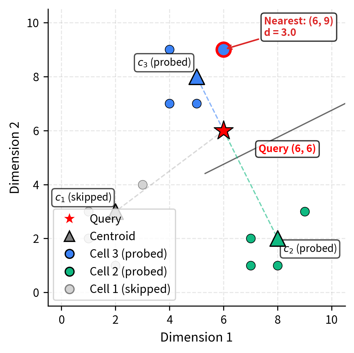
Let's walk through a concrete 2D example to ground the abstract concepts in tangible calculations. Working in two dimensions lets us follow every computation by hand and verify our geometric intuition. Suppose we have 12 vectors and partition them into clusters.
Training phase: K-means identifies three centroids. These are the points that minimize the within-cluster variance for their respective groups:
Assignment phase: Each vector is assigned to its nearest centroid, producing three inverted lists. Notice how the vectors in each cell are geographically close to their centroid. This is exactly the grouping property that makes IVF effective:
| Cell | Centroid | Vectors |
|---|
| 1 | | | | 2 | | | | 3 | | |
: Vector assignments to IVF cells after k-means clustering. {#tbl-ivf-assignments}
Each cell contains exactly 4 vectors, giving us perfectly balanced inverted lists. In practice, cells are rarely this uniform; the balance here makes the example easier to follow.
Query phase: A query arrives, and we set .
where is the query vector and means we will search the 2 cells whose centroids are closest to the query.
The first task is to determine which cells are most promising. We compute distances from the query to all centroids using Euclidean distance. The Euclidean distance between two 2D points and is:
where:
- : the coordinates of the first point
- : the coordinates of the second point
- : the sum of squared differences in each dimension
Taking the square root of this sum gives us the actual straight-line geometric distance and ensures the distance obeys the triangle inequality.
Applying this formula to each centroid, we can determine which regions of space are closest to our query:
where:
- : the Euclidean distance between the query vector and centroid
- : the query vector coordinates
- : the first centroid coordinates
- : the second centroid coordinates
- : the third centroid coordinates
Ranking these distances from smallest to largest, centroid is closest at distance 2.24, followed by centroid at distance 4.47, and finally centroid at distance 5.0. The two closest centroids are (distance 2.24) and (distance 4.47). With , we search the inverted lists for cells 3 and 2, scanning 8 of the 12 vectors. We skip cell 1 entirely, saving those 4 distance computations. In this small example, we save only 4 comparisons, but in a real dataset with millions of vectors and hundreds of centroids, this same principle eliminates the vast majority of distance computations.
Among the 8 vectors searched, the closest to is at distance 3.0 from cell 3:
where:
- : the vector from the scanned cells that is nearest to the query
- : the Euclidean distance calculation between query and result vector
- distance 3.0: the final computed distance
The zero contribution from the x-dimension shows the vector is directly above the query, differing only in the y-coordinate.
Note that if the actual nearest neighbor had been in cell 1 (which it isn't in this case), we would have missed it. This is the approximation trade-off. The decision to skip cell 1 was made based solely on centroid distances. While centroids are good summaries of their cells, they are not perfect predictors of which cell contains the nearest neighbor. In this example the approximation worked perfectly, but in general there is always a chance that a skipped cell harbors a closer vector, which is why increasing improves recall.
Code Implementation
Let's implement IVF search using FAISS, the library developed by Meta AI that provides highly optimized implementations of IVF and other index types. We'll also build a simple version from scratch to solidify the concepts.
Building IVF from Scratch
First, let's implement a minimal IVF index using NumPy and scikit-learn's k-means to understand the mechanics.
Now let's build the IVF index by training centroids and assigning vectors.
The average cell size indicates reasonably balanced partitioning. This balance is important because uneven cell sizes would make some probes substantially more expensive, creating unpredictable latency.
Now let's implement the query function.
Let's test this and compare against brute-force search.
The results demonstrate IVF's efficiency: searching 10-20% of the data achieves high recall (85-95%). Nearest neighbors cluster spatially, so examining a few cells captures most matches. Recall improvement diminishes with additional probes, revealing the characteristic accuracy-speed tradeoff curve.
Measuring Recall Across Many Queries
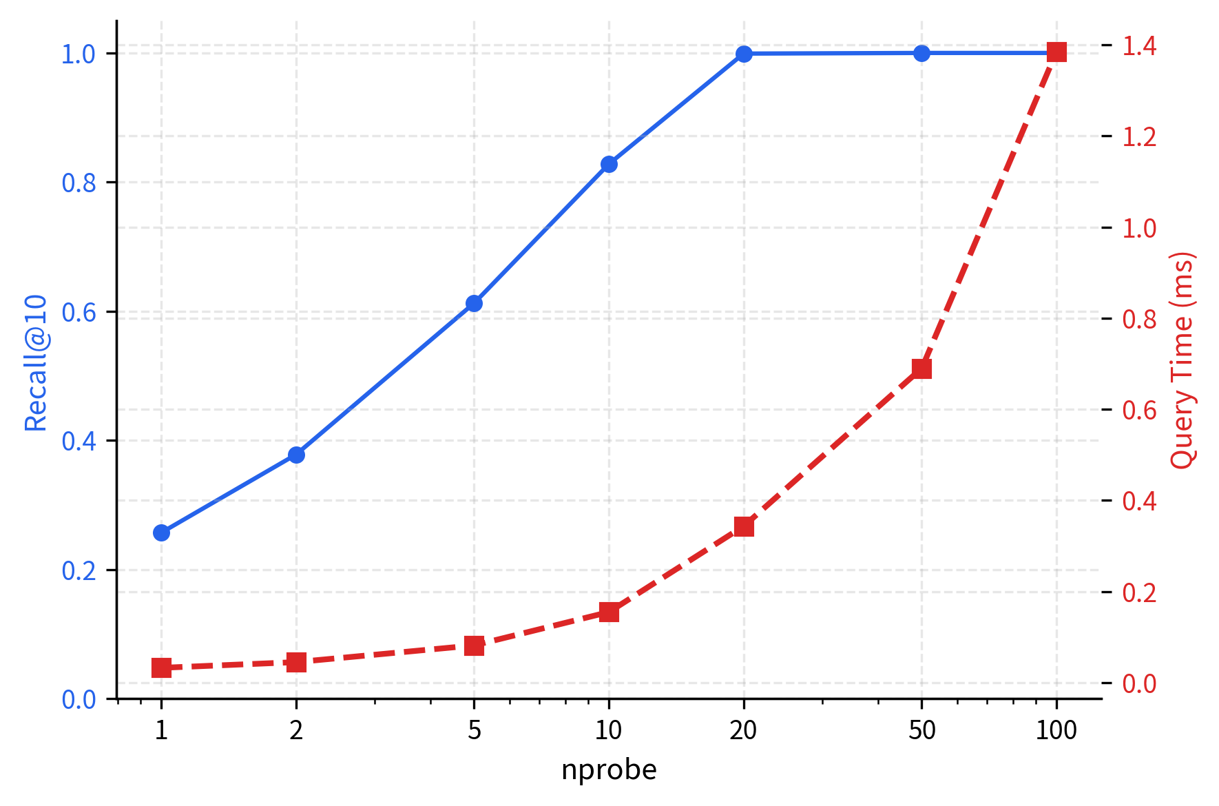
A single query can be misleading. Let's measure recall averaged over many queries to get a reliable picture of the accuracy-speed tradeoff.
The plot reveals the characteristic IVF tradeoff curve. Recall climbs steeply with the first few probes (the "easy" nearest neighbors are in the closest cells) then flattens as diminishing returns set in. Query time, meanwhile, grows linearly with since each additional cell adds a fixed number of vectors to scan.
Using FAISS for IVF
In practice, you'll use FAISS rather than a hand-rolled implementation. FAISS provides highly optimized IVF indexes with efficient memory management and multi-threaded search.
The output confirms successful index construction. The trained flag indicates that FAISS has learned the centroid positions through k-means clustering and is ready for queries. All vectors from the dataset have been successfully indexed and partitioned among the specified number of centroids.
Now let's search with different nprobe settings.
The results confirm that FAISS achieves the same recall-nprobe relationship as our scratch implementation, but with dramatically lower query times. The optimized C++ code and SIMD vectorization deliver 5-10x faster queries at the same accuracy levels, making FAISS the practical choice for production deployments.
Visualizing the Voronoi Partitioning
To build geometric intuition, let's visualize IVF in 2D.
This visualization reveals IVF's core efficiency: by comparing the query to centroids first, we identify the three most promising regions (blue, green, yellow). Only vectors in those cells are examined, while the majority of the dataset (gray points) is completely skipped. This spatial partitioning transforms an search into an search, delivering substantial speedups.
Choosing the Number of Centroids
The number of centroids affects both the granularity of the partitioning and the overhead of the centroid comparison step. To develop intuition for what happens when is set poorly, it helps to examine the two extremes. The choice involves several considerations.
Too few centroids (e.g., for 1 million vectors):
When the number of centroids is much too small relative to the dataset size, each cell becomes enormous. Each cell contains approximately:
where:
- : the total number of vectors in the dataset
- : the number of centroids (cells)
- : the average number of vectors per cell
With such large cells, even a single probe requires scanning 100,000 vectors, which offers minimal speedup over brute force. The cell is so large that it fails to meaningfully narrow down the search space.
Even with (searching just one cell), you scan:
where:
- : the fraction of cells searched when , approximating the fraction of the dataset examined
- : the number of centroids in this example
The centroid comparison step requires only distance computations, which is cheap. However, the list scanning step dominates since you must compute distances to 100,000 vectors. The problem is clear: the savings from coarse filtering are negligible because the cells are too coarse to filter effectively.
Too many centroids (e.g., for 1 million vectors):
At the opposite extreme, when we create far too many centroids, the cells become tiny and the overhead of simply finding the right cells becomes a bottleneck. Each cell contains approximately:
where:
- : the total number of vectors
- : the number of centroids, an excessive number for this dataset
- : the average number of vectors per cell, too small for efficient search
With cells this small, the true nearest neighbors are likely scattered across many cells, requiring a large to achieve good recall. The reason is geometric: when cells are very small, even a slight offset between the query and the nearest neighbor can place them in different cells. Additionally, comparing the query to 100,000 centroids itself becomes a bottleneck.
The centroid comparison step itself becomes expensive, and you need a very large to avoid missing nearby cells that contain true neighbors. The cost of Step 1 (finding nearest centroids) may even exceed the savings from Step 2 (scanning smaller lists) and defeat the purpose of the index entirely.
The right choice of lies between these extremes, at a point where both the centroid comparison cost and the list scanning cost are manageable. In practice, the guidelines for choosing are:
- Small datasets (): to
- Medium datasets (): to
- Large datasets ( to ): to
FAISS documentation recommends starting with between and and tuning from there based on your recall and latency requirements.
IVF-PQ: Combining Clustering with Compression
For very large datasets, even the vectors within each cell may not fit in memory. IVF can be combined with Product Quantization (PQ), a compression technique that represents each vector using compact codes instead of full floating-point values. We'll cover Product Quantization in detail in the next chapter, but the combination is important enough to preview here.
An IVF-PQ index combines IVF's space partitioning with Product Quantization's vector compression. Centroids identify which cells to search, and within each cell, vectors are stored as compressed PQ codes rather than full-precision vectors. This reduces memory by 10-50 while maintaining reasonable recall.
The FAISS implementation makes IVF-PQ straightforward to use:
The compression is dramatic. To appreciate just how much space is saved, we quantify the compression step by step, tracing the calculation from the original vector representation down to the compact PQ code.
Original vector size:
Each vector in float32 format requires 4 bytes per dimension. A 32-bit floating-point number can represent a continuous range of values with roughly 7 decimal digits of precision, which is the standard representation used in most machine learning frameworks:
where:
- : the dimensionality of each vector
- Factor of 4: bytes required for a float32 value (32 bits = 4 bytes)
This represents the uncompressed storage cost: every dimension requires a full floating-point number. For a dataset of one million vectors, this amounts to 256 megabytes just for the vector data alone.
PQ code size:
Product Quantization compresses each vector by dividing it into sub-vectors and encoding each with a single byte. Rather than storing 8 continuous floating-point values per sub-vector, PQ replaces each sub-vector with the index of the closest entry in a learned codebook. Since each index is a single byte, it can reference up to 256 different codewords.
where:
- : the number of sub-quantizers (sub-vectors) used in Product Quantization
- Each sub-quantizer uses 8 bits (1 byte) to encode its portion of the vector
Each byte can represent 256 () different values, so we're essentially replacing continuous dimensions with a single discrete code from a learned codebook. The codebook is learned during training and shared across all vectors, so its storage cost is amortized and negligible relative to the vector data.
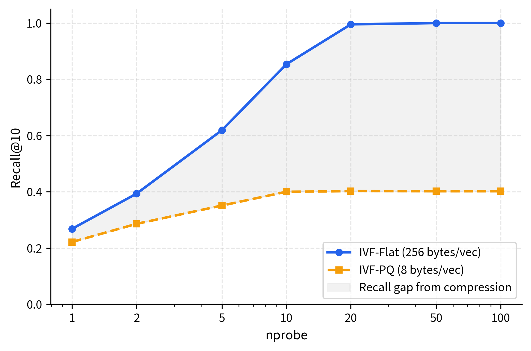
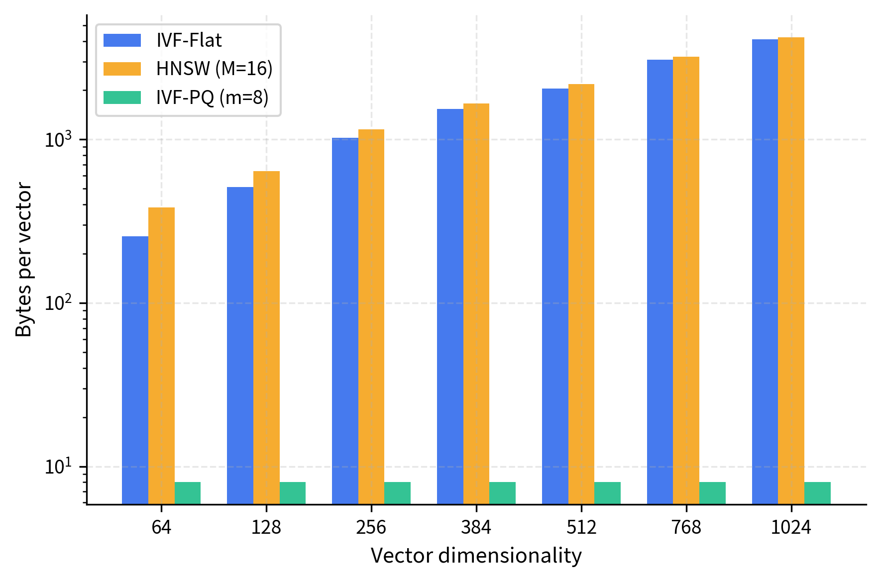
The PQ code represents the vector in just 8 bytes compared to the original 256 bytes, a compression factor of 32. The tradeoff is some loss in recall since PQ introduces quantization error in the distance computations. The distances computed from PQ codes are approximations of the true Euclidean distances, and this approximation error can cause some nearest neighbors to be ranked incorrectly.
The results show that IVF-PQ achieves strong recall (typically 90-95% of IVF-Flat's performance) while compressing vectors by 32x. This modest accuracy drop is well worth the dramatic memory savings and enables billion-scale deployments where storing full-precision vectors would be prohibitively expensive. The compression makes IVF-PQ the practical choice for very large collections. To quantify the scale: one billion vectors compressed to 8 bytes each requires only 8 GB of memory, versus 256 GB for uncompressed storage, making the difference between feasible and infeasible deployments.
The training cost increases with the number of vectors and the number of clusters. For a dataset of 10,000 vectors and 100 clusters, k-means typically converges within a few seconds on a modern laptop. For datasets with millions of vectors or hundreds of thousands of clusters, training can take minutes to hours. To speed up index construction, FAISS provides options like multi-threading and sampling-based k-means variants.
IVF vs HNSW
Both IVF and HNSW (covered in the previous chapter) are workhorses of approximate nearest neighbor search, but they make fundamentally different tradeoffs. Understanding when to use each one is critical for building effective RAG systems.
Structural Differences
HNSW builds a multi-layer proximity graph where each vector is a node connected to its approximate nearest neighbors. Search proceeds by greedy traversal from the top layer down. The graph structure must be stored alongside the vectors, adding memory overhead.
IVF partitions the space using clustering and stores vectors in inverted lists. Search identifies relevant clusters and scans their contents exhaustively. The overhead is just the centroids, which is minimal.
Memory Characteristics
HNSW requires storing the graph edges. With a typical parameter connections per node, each vector requires additional memory for graph storage. We calculate this overhead to understand the concrete cost.
Graph storage per vector:
Each node in the HNSW graph stores bidirectional connections, where each connection is represented by a 4-byte integer (the node ID). The bidirectionality means that if node A has an edge to node B, then node B also stores an edge back to node A. Both endpoints must record the connection so that the graph can be traversed efficiently in either direction during search:
The factor of 2 accounts for bidirectionality because in HNSW's implementation, each edge is stored at both endpoints to enable fast traversal in either direction. The factor of 4 comes from using 32-bit integers to store node IDs, which supports datasets of up to approximately 2 billion vectors.
where:
- : the maximum number of connections per node in the HNSW graph
- Factor of 2: accounts for bidirectional links, each edge stored twice (once at each endpoint)
- Factor of 4: bytes per integer, storing node IDs as 32-bit integers
This overhead is independent of vector dimensionality. Whether vectors are 64-D or 768-D, the graph structure costs the same per node. This is an important observation because it means the relative overhead of the graph decreases as vector dimensionality increases.
Overhead percentage for typical embeddings:
To understand whether 128 bytes per vector is significant, we need to compare it against the size of the vectors themselves. For 768-dimensional vectors (common in models like BERT) using 32-bit floats:
where:
- : the dimensionality of the embedding vectors
- : bytes per float32 value
- : the graph storage overhead per vector, calculated above
- : the total size of each 768-dimensional float32 vector in bytes
For higher-dimensional vectors, this percentage overhead decreases (graph cost stays constant while vector cost grows), making HNSW more attractive for very high-dimensional spaces. Conversely, for lower-dimensional vectors (say, 64 dimensions requiring only 256 bytes), the graph overhead of 128 bytes represents a 50% increase in memory, which is much more significant.
This overhead is modest, but the key constraint is that the entire graph structure must reside in memory for efficient traversal.
IVF stores centroids ( floats) and vector assignments, which is negligible overhead. More importantly, IVF naturally supports on-disk storage. The inverted lists can be memory-mapped, and only the lists being probed need to be loaded into memory. This makes IVF far more suitable for datasets that don't fit in RAM.
Speed Characteristics
HNSW typically offers better query latency for the same recall level, especially at high recall targets (>95%). The graph traversal naturally focuses on the relevant region of the space and adapts to the local density of the data. HNSW query time is also more predictable, as it doesn't depend on cell sizes.
IVF query time depends heavily on the uniformity of the clustering. If some cells are much larger than others (due to uneven data distributions), probing those cells is disproportionately expensive. However, IVF's simple structure makes it easier to parallelize. You can scan multiple inverted lists concurrently.
Index Construction
IVF requires a training phase (running k-means) before vectors can be added, but this training is relatively fast and adding new vectors is trivial (just assign them to the nearest centroid). Removing vectors is also straightforward.
HNSW builds incrementally. Each vector is inserted by finding its neighbors and adding edges. This can be slow for large datasets and the insertion order can affect quality. Deletion is also more complex because removing a node requires reconnecting its neighbors.
Practical Comparison
The following table summarizes the key tradeoffs:
| Characteristic | IVF | HNSW |
|---|---|---|
| Memory overhead | Low (centroids only) | Medium (graph edges) |
| Disk-friendly | Yes (memory-mapped lists) | No (requires RAM) |
| Query latency | Good | Better |
| Recall at low latency | Good | Better |
| Build time | Fast (k-means + assignment) | Slower (incremental insertion) |
| Update support | Easy add and remove | Easy add, hard remove |
| Scalability | Excellent (with PQ) | Good (limited by RAM) |
| Tuning complexity | Medium (, nprobe) | Medium (, ef) |
When to Use Which
Choose IVF when:
- Your dataset is too large to fit entirely in RAM
- You need to combine with Product Quantization for compression
- You need easy updates (adding/removing vectors frequently)
- You're operating at billion-scale
Choose HNSW when:
- Your dataset fits in memory
- You need the highest possible recall at low latency
- You can tolerate the memory overhead of the graph
- You have fewer than ~10 million vectors
In many production systems, the two approaches are combined. FAISS supports an IndexHNSW as the coarse quantizer in an IVF index, replacing the flat centroid comparison with an HNSW graph over the centroids. This provides fast centroid lookup when is very large.
Limitations and Impact
IVF's greatest strength is its simplicity, which is also the source of its main limitation. The quality of the partitioning depends entirely on how well k-means captures the structure of the data. K-means assumes roughly spherical, equally sized clusters. This assumption is rarely satisfied in real embedding spaces. High-dimensional embedding vectors often lie on complex manifolds where Euclidean clustering creates suboptimal boundaries. Vectors near the edges of their assigned cells are the most likely to be missed during search, and in high dimensions, a growing fraction of vectors sit near cell boundaries. This "boundary effect" means that IVF often needs higher values in high-dimensional spaces than you might expect from the ratio alone. One mitigation is to use more centroids, increasing the granularity of the partitioning and requiring correspondingly more probes. However, this increases both the centroid comparison cost and the training time.
Another practical limitation is that IVF requires a training step that sees a representative sample of the data before vectors can be indexed. This means you need a substantial number of vectors available upfront. If your data distribution shifts over time (for example, as new documents are added in a RAG system), the centroids may become stale and degrade recall. Periodic retraining is necessary in dynamic settings, which adds operational complexity compared to HNSW's incremental insertion model.
Despite these limitations, IVF remains one of the most widely deployed vector index structures. Its low memory overhead, natural compatibility with compression techniques like Product Quantization, and support for disk-based storage make it practical for large-scale retrieval. Nearly every major vector database, including Milvus, Pinecone, Weaviate, and Qdrant, offers IVF-based indexes. In the context of RAG systems, where you might need to search over millions of document chunks, IVF provides the scalability that makes dense retrieval feasible at production scale.
Summary
The IVF index partitions the vector space using k-means clustering, organizing vectors into cells defined by their nearest centroid. At query time, only the closest cells are searched, dramatically reducing the number of distance computations from to roughly . The key takeaways from this chapter are:
- Clustering as partitioning: K-means divides the space into Voronoi cells, and each cell maintains an inverted list of its member vectors. The number of centroids (typically between and , where is the number of vectors) controls the granularity of the partitioning.
- nprobe controls the tradeoff: Searching more cells improves recall but increases latency linearly. The sweet spot depends on your data distribution and accuracy requirements.
- IVF-PQ for scale: Combining IVF with Product Quantization compresses vectors from full precision to compact codes (often 8 to 32 bytes per vector) and enables billion-scale search with limited memory.
- IVF vs HNSW: IVF excels in large-scale, memory-constrained, and disk-based scenarios. HNSW provides better latency-recall tradeoffs when the dataset fits in memory. Many production systems use elements of both.
In the next chapter, we'll explore Product Quantization, understanding how it compresses high-dimensional vectors into compact codes while maintaining sufficient distance information for effective approximate search.
Key Parameters
The key parameters for IVF are:
- k (number of centroids): Controls the granularity of space partitioning. Typical values range from to where is the dataset size. More centroids create smaller cells but increase centroid comparison cost.
- nprobe: Number of cells to search at query time. Controls the accuracy-speed tradeoff. Higher values improve recall but increase query latency linearly.
- n_init: Number of k-means initializations during training. Higher values improve clustering quality but increase training time.
- max_iter: Maximum iterations for k-means convergence. Typical values are 20-300 depending on dataset size and convergence requirements.
Quiz
Ready to test your understanding? Take this quick quiz to reinforce what you've learned about IVF indexing for vector search.

Comments