Speculative Decoding Math: Algorithms & Speedup Limits

In the previous chapter, we introduced speculative decoding as a technique for accelerating autoregressive generation by having a small draft model propose multiple tokens that a larger target model verifies in parallel. The key insight was that verification is faster than sequential generation because it allows parallel processing. However, a critical question remains: how do we decide which draft tokens to accept?

The answer involves carefully designed acceptance criteria that guarantee mathematical correctness. We need a rejection sampling scheme that preserves the target model's output distribution exactly, not approximately. This chapter develops the mathematical framework for speculative decoding, including the acceptance criterion, expected speedup analysis, draft quality effects, and optimal draft length selection.

The fundamental challenge in speculative decoding is accepting draft tokens in a way that produces the exact same distribution as sampling directly from the target model. If we simply accept tokens when the draft and target models agree, we would bias the output toward the intersection of their distributions. Instead, we need a principled rejection sampling approach.

To understand the acceptance criterion, we must first appreciate the subtle problem it solves. When a draft model proposes a token, we face a fundamental question: how do we decide whether to keep that token while ensuring our final output looks exactly as if we had sampled directly from the target model? This is not merely about accepting "good" tokens and rejecting "bad" ones; it is about maintaining a precise mathematical relationship between what we accept and what the target model would have produced on its own.

Let $p(x)$ denote the target model's probability distribution over the next token, and let $q(x)$ denote the draft model's distribution. When the draft model proposes token $x$, we need an acceptance probability $\alpha(x)$ such that the final output distribution equals $p(x)$.

The key insight comes from rejection sampling, a classical technique in computational statistics that allows us to sample from one distribution by filtering samples from another. The fundamental idea is to sample from a "proposal" distribution (our draft model) and then selectively keep or reject those samples in a way that reshapes the distribution to match our target. If we accept with probability:

where:

• $\alpha(x)$: acceptance probability for token $x$
• $p(x)$: target model probability of token $x$
• $q(x)$: draft model probability of token $x$

then tokens where $p(x) \geq q(x)$ are always accepted, while tokens where $p(x) < q(x)$ are accepted with probability proportional to how much the target model favors them relative to the draft model.

To build intuition for this formula, consider what happens in two contrasting scenarios. In the first scenario, suppose the target model assigns probability 0.3 to token $x$ while the draft model only assigns probability 0.1. The ratio $p(x)/q(x) = 3$ exceeds 1, so we set $\alpha(x) = 1$ and always accept. This makes sense: the draft model is underproposing this token relative to what the target wants, so we should accept it whenever it appears. In the second scenario, suppose the target model assigns probability 0.1 to token $x$ while the draft model assigns probability 0.3. Now the ratio $p(x)/q(x) = 1/3$, so we accept with probability 1/3. The draft model is overproposing this token, so we need to reject some instances to bring its frequency down to what the target model expects.

Let's verify that this acceptance criterion produces the correct distribution. The verification proceeds through careful probability calculations that track what happens when we combine sampling from the draft model with our acceptance decision. When we sample $x \sim q(x)$ and accept with probability $\alpha(x)$, the probability of accepting a specific token $x$ is:

where:

• $P(\text{accept } x)$: probability of generating and accepting token $x$
• $q(x)$: probability of drafting token $x$
• $\alpha(x)$: probability of accepting drafted token $x$
• $p(x)$: probability of token $x$ under the target distribution

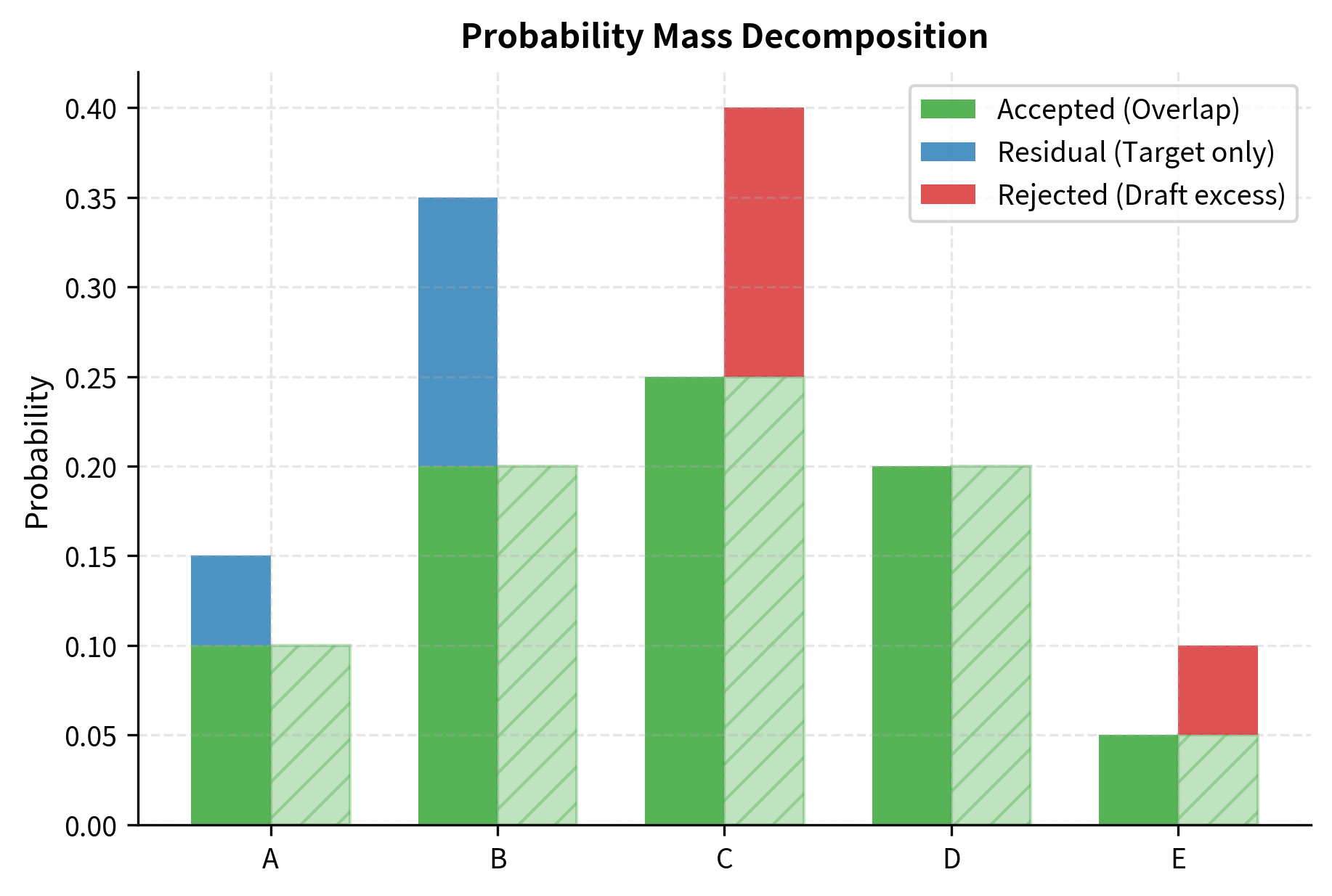
This derivation reveals that the probability of accepting any particular token $x$ is the minimum of the two distributions at that point. This creates a kind of "clipping" effect where we keep only the overlapping probability mass between the draft and target distributions.

The total acceptance probability across all tokens is:

where:

• $P(\text{accept})$: probability that a drafted token is accepted
• $\sum_x$: sum over the entire vocabulary
• $q(x)$: draft model probability of token $x$
• $p(x)$: target model probability of token $x$

This sum has a geometric interpretation. If you plot both distributions as histograms over the vocabulary, $P(\text{accept})$ equals the total area of overlap between the two histograms. When the distributions are identical, every token is accepted (total overlap equals 1). When they share no common support, no tokens are accepted (overlap equals 0).

Conditional on acceptance, the distribution over accepted tokens is:

where:

• $P(x \mid \text{accept})$: probability of token $x$ given it was accepted
• $\sum_{x'}$: normalization sum over all possible tokens $x'$
• $q(x)$: draft model probability
• $p(x)$: target model probability

This does not yet equal $p(x)$. The distribution is corrected by handling rejections appropriately.

When we reject a draft token, we don't simply redraft. Instead, we sample from a carefully constructed residual distribution that "fills in" the probability mass that rejection sampling missed. This residual distribution is the mathematical key that makes speculative decoding exact rather than approximate.

To understand why we need a residual distribution, consider what happens with pure rejection sampling. When we accept with probability $\min(q(x), p(x))$, we capture all the probability mass where the draft distribution meets or exceeds the target. But what about tokens where $p(x) > q(x)$? For these tokens, the draft model underestimates the target probability, and our rejection sampling only captures the portion up to $q(x)$. The residual distribution accounts for this missing mass.

Define:

where:

• $p_{\text{resid}}(x)$: residual distribution probability for token $x$
• $p(x)$: target model probability of token $x$
• $q(x)$: draft model probability of token $x$
• $p(x) - q(x)$: difference between target and draft probabilities
• $Z$: normalizing constant, $\sum_x \max(0, p(x) - q(x))$

The residual distribution captures the probability mass where $p(x) > q(x)$, which is exactly the mass that acceptance sampling misses. Geometrically, if you imagine the target distribution as a histogram and the draft distribution as another histogram overlaid on top, the residual distribution represents the portions of the target histogram that "stick out above" the draft histogram. By sampling from $p_{\text{resid}}$ on rejection, we ensure the overall distribution matches $p(x)$.

Notice that the normalizing constant $Z$ equals $1 - P(\text{accept})$, which is the total rejection probability. The probability mass captured by the residual distribution exactly equals the probability mass that rejection sampling misses, ensuring everything adds up correctly.

The full acceptance procedure for a single token position works as follows. This algorithm combines the acceptance criterion with the residual distribution to guarantee exact sampling from the target model:

1. Sample draft token $x \sim q(x)$
2. Sample uniform $u \sim \text{Uniform}(0, 1)$
3. If $u < \frac{p(x)}{q(x)}$, accept $x$
4. Otherwise, sample $x \sim p_{\text{resid}}(x)$

This procedure guarantees that the output follows distribution $p(x)$ exactly. To see why, consider that there are two mutually exclusive ways to generate a token $x$. The first path is through acceptance: we draft $x$ with probability $q(x)$ and accept it with probability $\min(1, p(x)/q(x))$, contributing $\min(q(x), p(x))$ to the total probability. The second path is through rejection and resampling: with probability $1 - P(\text{accept})$ we reject and then sample $x$ from the residual with probability $\frac{\max(0, p(x) - q(x))}{Z}$, contributing $\max(0, p(x) - q(x))$ to the total probability. Adding these two contributions gives $\min(q(x), p(x)) + \max(0, p(x) - q(x)) = p(x)$, exactly as desired.

In practice, the draft model proposes $k$ tokens at once. We verify them sequentially from left to right, accepting tokens until the first rejection. This sequential verification is essential because language models produce conditional distributions: the probability of each token depends on all preceding tokens.

Let $x_1, x_2, \ldots, x_k$ be the draft sequence. For position $i$, conditioning on the prefix $x_1, \ldots, x_{i-1}$:

where:

• $\alpha_i$: acceptance probability for the $i$-th token
• $x_i$: the $i$-th token in the draft sequence
• $p(x_i \mid \dots)$: target model conditional probability
• $q(x_i \mid \dots)$: draft model conditional probability

If position $i$ rejects, we sample from the residual distribution and discard positions $i+1, \ldots, k$. This maintains correctness because each accepted token was drawn from the correct conditional distribution. The key insight is that we cannot "skip" a rejection and continue verifying later tokens, because those tokens were conditioned on the rejected token. Once we sample a different token from the residual distribution, the entire subsequent sequence becomes invalid and must be regenerated.

This left-to-right verification creates an important efficiency consideration. Even though we verify all $k$ positions in a single parallel forward pass of the target model, we can only use tokens up to the first rejection. However, because we always sample from the residual distribution upon rejection, we are guaranteed to produce at least one valid token per iteration, even if all $k$ draft tokens are rejected. In fact, when all tokens are accepted, we get $k + 1$ tokens, since the target model's forward pass also provides the distribution for the next position beyond the draft sequence.

Understanding the expected speedup from speculative decoding requires analyzing how many tokens we expect to accept from each draft sequence and how this translates to wall-clock improvements. This analysis provides both theoretical insights and practical guidance for deploying speculative decoding systems.

Let $\alpha$ denote the average acceptance probability for a single token. Under simplifying assumptions where each position has the same acceptance rate, we can derive a clean expression for this probability. While real-world acceptance rates vary by position and context, this i.i.d. assumption provides valuable analytical insights.

where:

• $\alpha$: expected acceptance probability
• $\mathbb{E}_{x \sim q}$: expectation over tokens proposed by the draft model
• $q(x)$: draft model probability of token $x$
• $p(x)$: target model probability of token $x$
• $\sum_x \min(q(x), p(x))$: overlap between the two distributions

This quantity measures the overlap between the draft and target distributions. When the distributions are identical, $\alpha = 1$. When they are completely disjoint, $\alpha = 0$. In practice, $\alpha$ typically falls between 0.6 and 0.9 for well-matched draft and target model pairs.

Given a draft of length $k$, the number of accepted tokens follows a truncated geometric distribution. This distribution arises because we accept tokens sequentially until the first rejection, but we stop at position $k$ even if no rejection has occurred. Let $N$ be the number of tokens we generate (accepted drafts plus one from rejection sampling or the $(k+1)$th position). The expected value is:

where:

• $\mathbb{E}[N]$: expected number of accepted tokens (plus one verification)
• $k$: draft sequence length
• $\alpha$: probability of accepting a single token
• $i$: position of the first rejection
• $\alpha^{i-1}(1-\alpha)$: probability that the first rejection occurs at position $i$
• $(k+1) \cdot \alpha^k$: contribution from the case where all $k$ tokens are accepted

The first term accounts for rejecting at position $i$ (we keep $i$ tokens including the resampled one). The second term accounts for accepting all $k$ drafts (we get $k+1$ tokens including the bonus verification token).

We can simplify this sum by observing that $N$ is 1 plus the count of accepted draft tokens. Since the probability of accepting the first $j$ tokens is $\alpha^j$ for all $j \le k$ (under the simplified i.i.d. assumption), we can use the linearity of expectation:

where:

• $\mathbb{E}[N]$: closed-form expected number of tokens generated per iteration
• $\alpha$: acceptance probability
• $k$: draft length

This closed-form expression shows that expected tokens per iteration grow as a geometric series in the acceptance probability. When $\alpha$ is close to 1, almost all draft tokens are accepted, and $\mathbb{E}[N]$ approaches $k+1$. When $\alpha$ is close to 0, most drafts are rejected immediately, and $\mathbb{E}[N]$ approaches 1 (we generate just one token from the residual distribution).

Let $c$ be the cost ratio, defined as the time for one target model forward pass divided by the time for one draft model forward pass. Typically $c \gg 1$ since the target model is much larger. For example, if the target model has 70 billion parameters and the draft model has 7 billion parameters, we might expect $c$ to be roughly 10, depending on hardware and batching configurations.

Without speculative decoding, generating $n$ tokens requires $n$ target model passes, taking time $n \cdot T_{\text{target}}$.

With speculative decoding, each iteration requires:

• One draft model pass generating $k$ tokens, taking time $k \cdot T_{\text{draft}}$
• One target model pass verifying all $k$ positions, taking time $T_{\text{target}}$

The iteration produces $\mathbb{E}[N] = \frac{1 - \alpha^{k+1}}{1 - \alpha}$ tokens on average and takes time $T_{\text{target}} + k \cdot T_{\text{draft}} = T_{\text{target}}(1 + k/c)$.

The speedup ratio $S$ compares how fast we generate tokens with speculative decoding versus standard autoregressive generation. We derive this by computing the time per token under both approaches:

where:

• $S$: speedup ratio
• $T_{\text{target}}$: time for standard autoregressive generation per token
• $k$: draft length
• $c$: cost ratio ($T_{\text{target}} / T_{\text{draft}}$)
• $\alpha$: acceptance probability (used in $\mathbb{E}[N]$)
• $1 + k/c$: cost of one speculative iteration in units of target model passes
• $\mathbb{E}[N]$: average tokens produced per iteration

This formula captures the essential tradeoff in speculative decoding. The numerator measures benefit, specifically how many tokens we expect to generate per iteration. The denominator measures cost, specifically how much computation that iteration requires. Speedup greater than 1 means speculative decoding is faster than standard generation.

When the draft model is very fast ($c \to \infty$), this simplifies to:

where:

• $S$: theoretical maximum speedup with a zero-cost draft model
• $\alpha$: acceptance probability
• $k$: draft length

This limiting case represents the best possible speedup when the draft model adds negligible overhead. In practice, draft models incur costs, so the actual speedup is lower than this bound. However, this formula provides a useful upper limit for what speculative decoding can achieve.

The acceptance probability $\alpha$ directly depends on how well the draft model approximates the target model. Understanding this relationship helps us choose appropriate draft models and predict performance. The choice of draft model is a critical practical decision in deploying speculative decoding.

Draft quality can be quantified by the expected acceptance probability:

where:

• $\alpha$: measure of draft quality (higher is better)
• $q(x)$: draft distribution
• $p(x)$: target distribution

This quantity has a clear interpretation: it is the probability mass that the two distributions share. A high-quality draft model assigns similar probabilities to most tokens as the target model, resulting in large overlap. A poor draft model might assign high probability to tokens the target model dislikes, or vice versa, resulting in small overlap.

This is related to the total variation distance between distributions, one of the most fundamental measures of dissimilarity between probability distributions:

where:

• $TV(p, q)$: total variation distance
• $p(x)$: target distribution probability for token $x$
• $q(x)$: draft distribution probability for token $x$
• $|p(x) - q(x)|$: absolute difference in probability for token $x$
• $\alpha$: acceptance probability

Higher draft quality means smaller total variation distance, which means higher acceptance probability. This connection to total variation distance indicates that the acceptance probability captures the most fundamental notion of distributional similarity: the maximum probability that an adversary could distinguish between samples from the two distributions.

Larger draft models tend to produce distributions closer to the target, increasing $\alpha$. However, larger models are slower, decreasing $c$. The optimal draft model balances these factors, and finding this balance requires understanding the tradeoffs involved.

Consider three scenarios:

• Very small draft model: Fast inference ($c$ large) but poor distribution match ($\alpha$ small). We accept few tokens per iteration, limiting speedup. As a concrete example, imagine using a tiny 125M parameter model as the draft for a 70B parameter target. The draft model runs 100 times faster than the target, but it might only match the target's distribution 40% of the time. Most iterations produce just one or two tokens before rejection.

• Medium draft model: Moderate speed and moderate acceptance rate. Often the sweet spot for practical applications. A 7B draft model for a 70B target might run 10 times faster while achieving 75% acceptance rates. This combination often yields the highest speedups in practice.

• Large draft model: Good distribution match ($\alpha$ close to 1) but slow ($c$ small). The overhead of running the draft model eats into speedup gains. A 30B draft for a 70B target might achieve 90% acceptance rates, but if it only runs 2-3 times faster than the target, the iteration cost is too high to achieve meaningful speedup.

In practice, acceptance rates typically range from 0.6 to 0.9 depending on:

• Model family similarity (using a smaller model from the same family yields higher $\alpha$)
• Task difficulty (easier, more predictable text has higher $\alpha$)
• Temperature settings (lower temperature often increases $\alpha$)

These factors interact in interesting ways. For instance, at very low temperatures where sampling becomes nearly deterministic, both draft and target models tend to select the same highest-probability token, resulting in acceptance rates approaching 1. At higher temperatures where sampling explores more of the distribution, the models are more likely to disagree, reducing acceptance rates.

Choosing the draft length $k$ involves balancing the cost of generating more drafts against the diminishing probability of accepting them all. This optimization problem has both theoretical and practical importance.

We want to find $k^*$ that maximizes speedup:

where:

• $k^*$: optimal draft length
• $\mathbb{E}[N_k]$: expected tokens generated with draft length $k$
• $c$: cost ratio

Taking the derivative with respect to $k$ and setting to zero is analytically intractable, but we can understand the behavior through analysis of the numerator and denominator.

The expected tokens $\mathbb{E}[N_k]$ grows sublinearly in $k$:

where:

• $\mathbb{E}[N_k]$: expected tokens for draft length $k$
• $\frac{1}{1-\alpha}$: asymptotic limit of expected tokens
• $\alpha < 1$: acceptance probability

The growth rate decreases exponentially because $\alpha^k$ decays exponentially. Meanwhile, the cost $1 + k/c$ grows linearly in $k$. This tension creates an interior optimum. Intuitively, each additional draft token has a diminishing marginal benefit (it is only useful if all previous tokens were accepted, which becomes increasingly unlikely) but a constant marginal cost (one more draft model forward pass). At some point, the marginal cost exceeds the marginal benefit, and we should stop drafting.

For large $c$ (fast draft model), we can derive an approximate optimal draft length. When $c \to \infty$, the optimal $k$ is infinite since there's no cost to drafting more tokens. For finite $c$, the optimal $k$ satisfies:

where:

• $\frac{d}{dk}$: derivative with respect to draft length $k$
• $\alpha$: acceptance probability
• $c$: cost ratio
• The expression in brackets is the speedup function

Applying the quotient rule for differentiation:

where:

• $\alpha$: acceptance probability
• $k$: draft length
• $c$: cost ratio
• $-\alpha^{k+1} \ln(\alpha)$: derivative of the numerator term $(1 - \alpha^{k+1})$
• $1/c$: derivative of the denominator term $(1 + k/c)$
• $(1 + k/c)^2$: squared denominator from the quotient rule

Setting the numerator to zero gives:

where:

• $\alpha$: acceptance probability
• $k$: draft length
• $c$: cost ratio
• $-\alpha^{k+1} \ln(\alpha)$: marginal gain term
• Right side: marginal cost term

This equation balances marginal benefit against marginal cost. The left side represents the expected additional tokens from extending the draft by one position. The right side represents the cost of that extension in terms of reduced speedup per existing token. While this equation cannot be solved in closed form, it can be solved numerically for any specific values of $\alpha$ and $c$.

For typical values ($\alpha \approx 0.7$, $c \approx 10$), optimal $k$ ranges from 4 to 8 tokens.

In practice, the optimal $k$ varies based on context. Some systems use adaptive strategies:

• Fixed $k$: Simple to implement, works well when acceptance rates are stable
• Adaptive $k$: Adjust based on recent acceptance rates
• Tree-based drafting: Generate multiple candidate continuations, increasing effective acceptance probability

The adaptive approach monitors acceptance rates during generation and increases $k$ when rates are high (indicating the draft model is performing well on the current content) or decreases $k$ when rates are low (indicating more challenging content where longer drafts would be wasteful).

Let's implement the speculative decoding mathematics to see these concepts in action.

First, we'll implement the acceptance criterion for a single token:

Let's verify that this produces the correct distribution:

The empirical distribution closely matches the target, confirming our acceptance criterion preserves the correct distribution.

Now let's calculate expected speedup for different configurations:

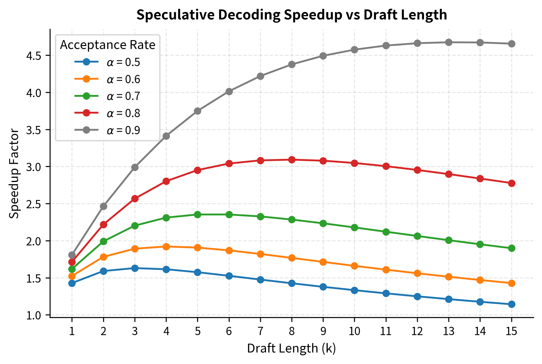
Let's visualize how speedup varies with draft length for different acceptance rates:

The plot shows that optimal draft length increases with acceptance probability. For $\alpha = 0.9$, we can productively use 8-10 draft tokens, while $\alpha = 0.5$ shows diminishing returns after just 3-4 tokens.

Let's find the optimal $k$ for different scenarios:

The results confirm our analysis: higher acceptance rates and faster draft models (larger $c$) support longer draft sequences and achieve greater speedup.

Finally, let's visualize the acceptance rate as a function of distribution similarity:

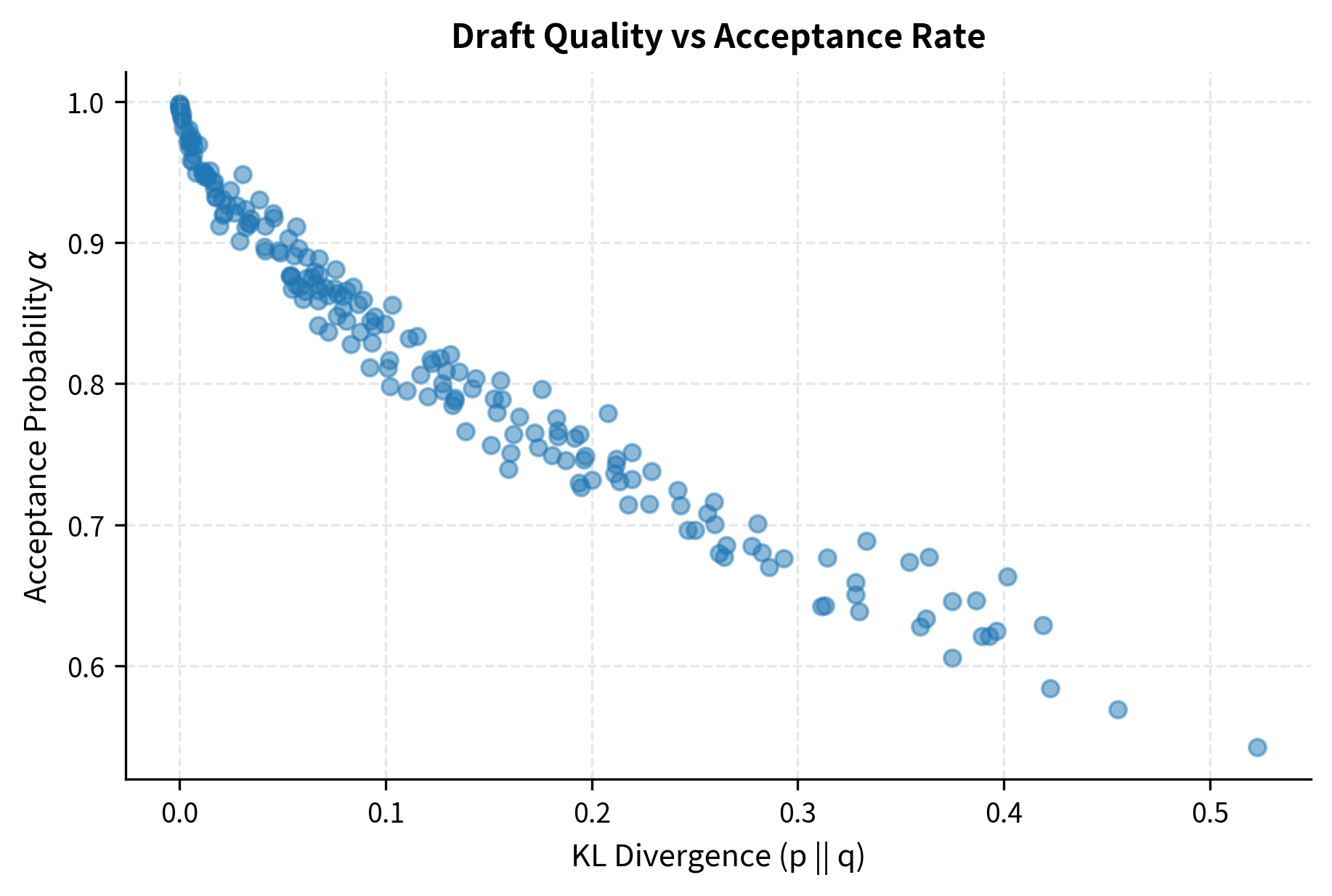
The relationship between distribution divergence and acceptance probability is clear: as the draft model's distribution diverges from the target, acceptance rates drop substantially. This underscores the importance of choosing draft models that approximate the target well.

The key parameters for the speculative decoding implementation are:

• k: Draft length. The number of tokens proposed by the draft model in each step.
• c: Cost ratio ($T_{\text{target}} / T_{\text{draft}}$). Represents how much faster the draft model is compared to the target model.
• alpha: Acceptance probability ($\alpha$). The probability that a draft token is accepted by the target model, derived from distribution overlap.

While the mathematics of speculative decoding provides strong theoretical guarantees, several practical challenges affect real-world performance.

The acceptance criterion assumes we can efficiently compute both $p(x)$ and $q(x)$ for all tokens. In practice, this means running the full forward pass of both models, even though we only need the probability of specific draft tokens. Some implementations optimize this by caching intermediate states, but the full softmax computation remains a bottleneck. The residual distribution sampling also requires computing the full target distribution, making it difficult to apply speculative decoding with certain memory-efficient generation techniques.

The i.i.d. assumption in our speedup analysis rarely holds in practice. Acceptance rates vary significantly based on context: function names and common phrases have high acceptance rates, while creative or technical content sees more rejections. This variance means actual speedups may differ from theoretical predictions, and systems should monitor acceptance rates to adapt draft lengths dynamically. Additionally, the tree-structured extensions to speculative decoding (generating multiple candidate continuations) can improve effective acceptance rates but add implementation complexity.

Hardware considerations also affect practical speedup. The theoretical model assumes draft and target passes don't interfere with each other's memory or compute. On GPUs with limited memory bandwidth, loading both models' weights can create contention. Some deployments use separate GPUs for draft and target models, while others time-multiplex on a single device. Continuous batching systems, which we'll explore in the next chapter, add another layer of complexity to speculative decoding integration.

This chapter developed the mathematical foundations of speculative decoding, providing tools to understand and optimize this important inference acceleration technique.

The acceptance criterion uses rejection sampling with a residual distribution to guarantee that speculative decoding produces outputs identical in distribution to standard autoregressive sampling. The acceptance probability $\alpha(x) = \min(1, p(x)/q(x))$ ensures we accept tokens where the draft model underestimates the target probability while probabilistically rejecting overestimated tokens.

Expected speedup depends on the acceptance probability $\alpha$, draft length $k$, and cost ratio $c$. The formula $S = \frac{(1 - \alpha^{k+1})/(1-\alpha)}{1 + k/c}$ captures the tradeoff between generating more draft tokens and the diminishing probability of accepting them all.

Optimal draft length balances these factors. Higher acceptance rates support longer drafts, with practical optima typically ranging from 4 to 10 tokens depending on model quality and hardware configuration.

Draft model quality directly impacts speedup through the acceptance probability $\alpha = \sum_x \min(p(x), q(x))$. Smaller models within the same family often provide the best balance of speed and distribution similarity.

Ready to test your understanding? Take this quick quiz to reinforce what you've learned about speculative decoding math.