

Discover how continuous batching achieves 2-3x throughput gains in LLM inference through iteration-level scheduling, eliminating static batch inefficiencies.

This article is part of the free-to-read Language AI Handbook
Choose your expertise level to adjust how many terms are explained. Beginners see more tooltips, experts see fewer to maintain reading flow. Hover over underlined terms for instant definitions.
Continuous Batching
Large language model inference presents a unique challenge that sets it apart from nearly every other machine learning workload: requests arrive at different times, require different numbers of output tokens, and finish at unpredictable moments Traditional batch processing, borrowed from training workflows where uniformity is the norm, handles this reality poorly. A batch must wait for its slowest member, leaving GPU resources idle while fast requests sit completed but unable to exit. The result is a system that wastes expensive compute cycles and frustrates you when you expect snappy responses.
Continuous batching solves this fundamental mismatch by rethinking how we group work together. Rather than treating a batch as a monolithic unit processed as a single group, continuous batching treats each decoding iteration as an opportunity to reshuffle which requests are actively using compute. Completed requests exit immediately, and waiting requests join without delay.
This chapter explores why static batching creates inefficiency, how continuous batching addresses it through iteration-level scheduling, and the mechanisms for handling request completion. The throughput gains from this approach are substantial, often doubling or tripling the requests per second a single GPU can handle. Understanding continuous batching is essential for when you deploy language models in production, as it has become the standard technique in modern serving frameworks.
The Batching Problem in LLM Inference
Batching multiple requests together is essential for efficient GPU utilization. Modern GPUs contain thousands of processing cores designed to execute operations in parallel, and feeding them work one request at a time leaves most of this capability unused. As we discussed in the KV Cache chapter, autoregressive generation produces one token per forward pass. Each forward pass involves substantial overhead: loading model weights from memory, executing attention computations, and applying the feed-forward network. Without batching, each forward pass processes a single request, leaving most of the GPU's parallel processing capability unused. Matrix multiplications that could operate on batch sizes of 32 or 64 instead operate on a single row, significantly underutilizing the thousands of available cores.
Training workflows batch naturally because all samples pass through the same computation graph with identical sequence lengths (after padding). Every example in a training batch starts together, processes together, and finishes together. This uniformity makes scheduling trivial. Inference is different in three critical ways that break this simple model:
- Variable input lengths, requests arrive with prompts of different sizes. You might submit a 10-token question while another provides a 2000-token document for summarization.
- Variable output lengths: Some responses are 10 tokens, others are 1000. A simple factual answer completes quickly, while a detailed explanation continues for many iterations.
- Asynchronous arrivals: Requests come in continuously, not in neat batches. You submit queries at unpredictable times, and the system cannot wait indefinitely to form perfect batches.
These differences create a fundamental tension between batching efficiency and response latency. We want large batches to maximize GPU utilization, but we also want to return responses quickly without waiting for other requests.
Static Batching
The simplest approach to batching inference requests is static batching, where we collect a fixed group of requests, process them together until all complete, and then start the next batch. This approach mirrors how training works and requires minimal changes to existing infrastructure.
How Static Batching Works
In static batching, the system follows a straightforward process that prioritizes simplicity over flexibility. The core idea is to treat a batch as an indivisible unit that processes from start to finish without any changes to its composition. This makes implementation easy but creates significant inefficiencies when requests have different characteristics.
The static batching algorithm proceeds through five distinct phases:
- Accumulate requests. Wait until a batch of size requests arrives, or a timeout expires. During this phase, incoming requests queue up while the system decides whether enough work has accumulated to justify starting a new batch.
- Pad to uniform length. Pad all input sequences to match the longest input in the batch. Since matrix operations require uniform dimensions, shorter sequences receive padding tokens that consume compute but produce no useful output.
- Process together. Run all requests through every decoding iteration. The entire batch moves in lockstep, with each request generating one token per forward pass.
- Wait for completion. Continue until the longest output sequence finishes. Even if some requests complete after just a few tokens, they remain in the batch, consuming resources while producing only padding.
- Return results. Send all responses back and start the next batch. Only after every request has finished can the system collect a new batch and begin again.
Let's see how static batching performs with requests of varying output lengths. This simulation demonstrates the core problem: when requests differ significantly in how many tokens they need to generate, the short requests end up waiting for the long ones.
The Efficiency Problem
The analysis reveals the core problem with static batching: requests that finish early continue consuming compute resources. In our example, some requests only needed around 20 tokens while the batch waited for requests generating nearly 200 tokens. Those short requests sat idle for over 150 iterations, wasting computational resources that could have been serving you.
To understand why this matters, consider what happens inside the GPU during those wasted iterations. The completed request still occupies a slot in every tensor operation. The attention mechanism still computes over its position. The feed-forward network still processes its hidden state. The output is discarded as padding, but the compute is very real. This is not idle waiting; it is inefficient computation.
This inefficiency compounds across several dimensions:
- Memory waste. Completed requests retain their KV cache entries until the batch finishes. As we covered in the KV Cache Memory chapter, each request's cache can consume gigabytes of GPU memory. A 7B parameter model might need 1-2 GB per request at full context length. Keeping completed requests' caches prevents new requests from starting, creating a bottleneck even when compute capacity exists.
- Latency inflation. Short requests experience artificially high latency because they must wait for longer siblings in their batch. A 20-token response that takes 100ms to generate might not be returned for 1000ms while waiting for a 200-token sibling. From your perspective, this feels like unexplained slowness, damaging your experience even though the system technically completed your request quickly.
- GPU underutilization. As requests complete, effective batch size shrinks. A batch starting with 8 requests might have only 2 active requests for its final iterations, dramatically reducing throughput. The GPU cores that could be serving new requests instead sit mostly idle, processing padding tokens for the few remaining active sequences.
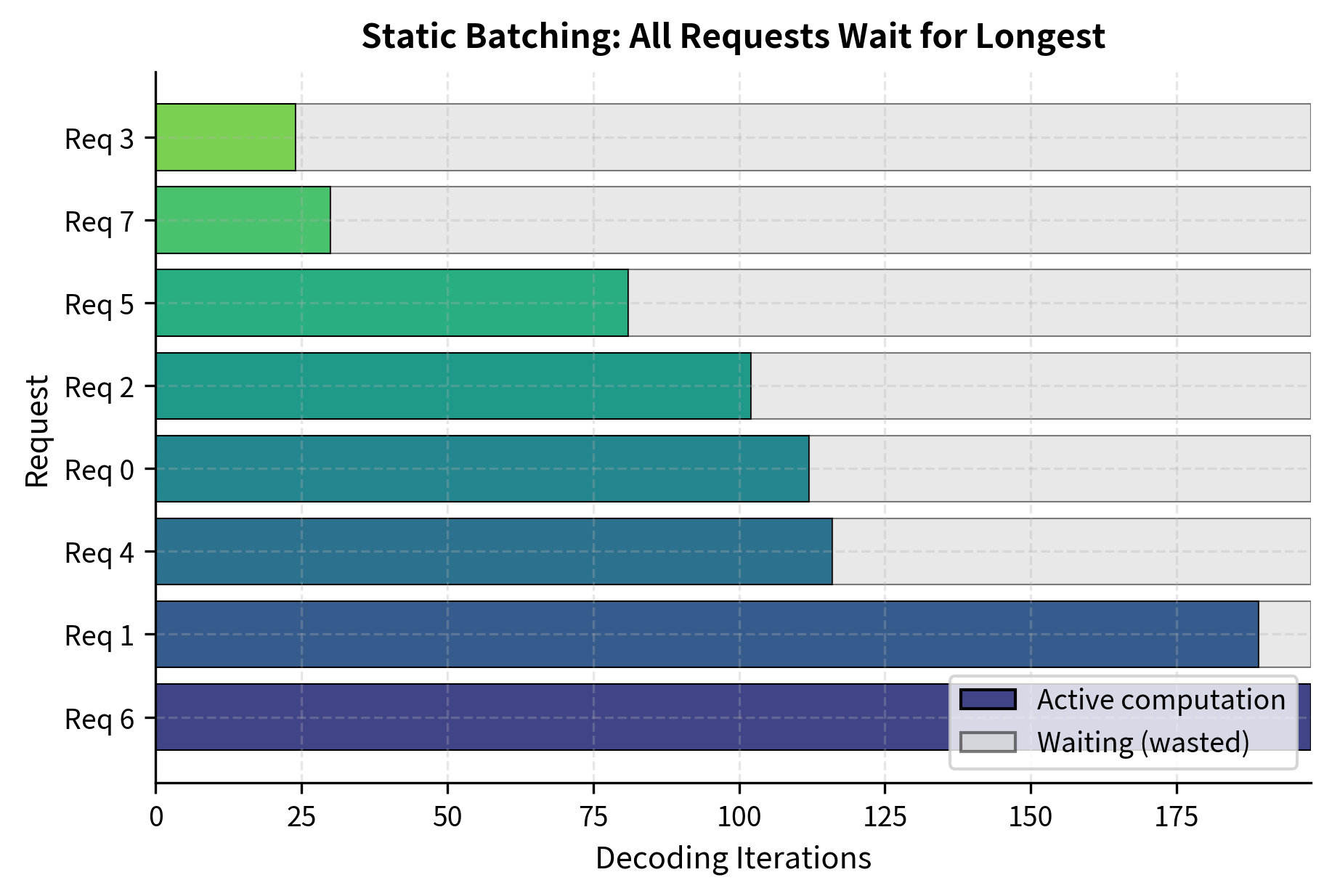
The gray regions in this visualization represent wasted computation: the GPU performs forward passes that produce padding tokens, while the finished requests cannot release their resources. The shorter the original request, the larger the fraction of its total batch time spent waiting.
Continuous Batching
Continuous batching, also called iteration-level scheduling or in-flight batching, takes a fundamentally different approach to managing concurrent requests. Instead of treating a batch as a fixed unit that lives and dies together, it treats each decoding iteration as an independent scheduling decision. This seemingly simple change significantly improves both throughput and latency.
The Core Insight
The key insight behind continuous batching emerges from a careful examination of how autoregressive generation actually works. Each decoding step produces exactly one token per request. Between any two decoding iterations, the model completes one forward pass and begins the next. At this boundary, we have complete freedom to reorganize which requests participate in the next iteration. The model does not care whether the same requests continue; it only needs valid input tokens and their associated KV caches.
This observation reveals that the rigid batch structure of static batching is entirely artificial. There is no technical requirement that forces us to keep completed requests around. We imposed that constraint for implementation simplicity, not because the underlying computation demands it.
With this insight, continuous batching introduces three powerful capabilities:
- Remove completed requests. Immediately release slots when requests hit their end token. The moment a request generates its end-of-sequence marker, it exits the batch and its resources become available.
- Add new requests. Insert waiting requests into freed slots. New requests join the batch at whatever iteration happens to have space, rather than waiting for a complete batch turnover.
- Maintain continuous flow. Keep the batch saturated with active work. The goal is to maintain maximum occupancy at all times, treating the batch like a continuously flowing river rather than a series of discrete buckets.
This transforms batch processing from a rigid structure into a dynamic queue where requests flow through the system at their natural pace. Short requests complete quickly and exit. Long requests continue as needed. New requests enter as soon as space permits.
How Continuous Batching Works
The continuous batching algorithm operates in a perpetual loop that never truly stops between batches. Instead of collecting requests, processing them, and collecting again, it maintains a persistent set of active requests that evolves iteration by iteration. Each cycle through the loop represents a single forward pass through the model.
The algorithm follows these steps in each iteration:
- Check for completions. After each iteration, identify requests that generated an end-of-sequence token or reached their maximum length. These requests have finished their work and no longer need to participate.
- Evict completed requests. Remove finished requests from the active batch, freeing their slots and KV cache memory. This happens immediately, not at some future batch boundary.
- Check waiting queue. Look for pending requests that arrived while the batch was processing. New requests accumulate in a queue whenever all slots are occupied.
- Insert new requests. Fill empty slots with waiting requests, running their prefill phase to build initial KV caches. These new requests join alongside existing decode phase requests.
- Execute iteration. Run one decoding step for all active requests. Every active request generates exactly one token.
- Return completed results. Send finished responses back to clients immediately. You receive your results the moment generation completes, not when some arbitrary batch finishes.
Let's simulate the same requests with continuous batching to see the difference in practice:
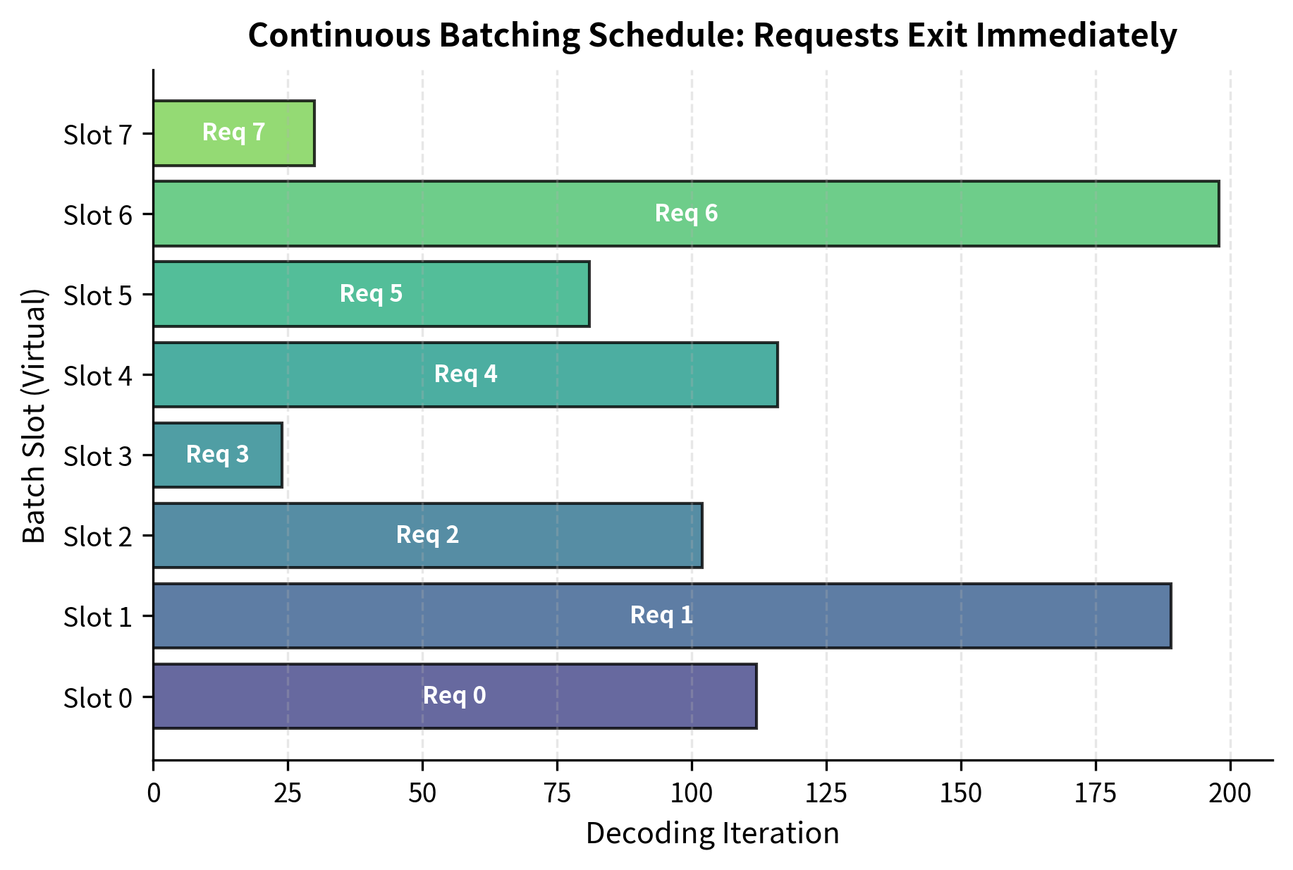
The high utilization and reduced iteration count demonstrate how continuous batching effectively saturates the GPU. By immediately filling slots vacated by completed requests, the system minimizes idle time and approaches the theoretical maximum throughput for the given workload. Notice that the total iterations is much closer to the theoretical minimum than what static batching achieved.
Iteration-Level Scheduling
The power of continuous batching comes from making scheduling decisions at every iteration. Rather than committing to a fixed plan when a batch starts, the system reevaluates its choices thousands of times per second. This fine-grained control enables sophisticated policies beyond simple FIFO (first-in-first-out) ordering and allows the system to adapt dynamically to changing conditions.
Scheduling Decisions
At each iteration boundary, the scheduler faces several interconnected decisions that determine both throughput and fairness. These decisions happen in microseconds and must balance competing objectives.
Which requests to evict: Besides naturally completed requests, the scheduler might preempt requests to free memory for higher-priority work. This creates interesting tradeoffs between fairness and throughput. A request that has already consumed significant resources represents sunk cost, but continuing it also delays new requests. The scheduler must weigh these factors according to the system's priorities.
Which waiting requests to admit: When multiple requests are waiting, the scheduler chooses which to start first. This decision significantly impacts your perceived latency and overall system efficiency. Options include:
- FIFO. First-come, first-served, which is simple and fair. Every request eventually gets its turn in the order it arrived. This approach provides predictable behavior and prevents starvation.
- Shortest Job First. Prioritize requests with shorter expected outputs to minimize average latency. Short requests complete quickly, improving your experience. However, this requires predicting output length, which is not always possible.
- Priority-based. Honor explicit priority levels attached to requests. You or time-sensitive applications might receive preferential treatment. This approach requires clear policies about what constitutes priority.
How to handle memory pressure: When the KV cache approaches capacity, the scheduler must decide whether to wait for completions or preempt active requests. Waiting reduces throughput but preserves work in progress. Preemption frees resources immediately but wastes the computation already invested in the preempted request.
Prefill and Decode Phases
Continuous batching must handle requests in different phases of their lifecycle. As we discussed in the KV Cache chapter, generation has two distinct phases with fundamentally different computational characteristics.
- Prefill phase. Process all input tokens in parallel to build the initial KV cache. This phase is compute-bound and benefits from large batch sizes of tokens. The GPU performs dense matrix multiplications over potentially thousands of input tokens, fully utilizing its computational capacity. Memory bandwidth is not the bottleneck during prefill because the computation is so intensive.
- Decode phase. Generate tokens one at a time, reading from the KV cache. This phase is memory-bandwidth-bound and benefits from large batch sizes of requests. Each decode step reads the entire KV cache but performs relatively little computation per byte loaded. The GPU spends most of its time waiting for memory, not computing.
These phases have different computational characteristics that create challenges when mixing them in the same batch. Prefill processes many tokens per request; decode processes one token per request. Mixing them creates load imbalance: prefill requests demand heavy compute while decode requests sit largely idle, waiting for memory operations to complete.
Chunked Prefill
Modern continuous batching systems often use chunked prefill to better balance the two phases and smooth out the computational load. Instead of processing the entire prompt in one iteration, which can cause latency spikes when long prompts arrive, long prompts are split into manageable chunks.
The chunking strategy divides a long prompt into pieces that can be processed incrementally. This allows decode iterations for other requests to proceed between prefill chunks, maintaining responsiveness for you. A request with a 3000-token prompt might be split into six chunks of 500 tokens each, with each chunk processed in a separate iteration.
Chunked prefill enables interleaving decode tokens between prefill chunks, reducing latency spikes when long prompts arrive. Without chunking, a 3000-token prompt would monopolize the GPU for a significant duration, blocking all decode operations for other requests. With chunking, decode operations proceed smoothly while the long prompt is processed incrementally.
Request Completion Handling
Handling completed requests efficiently is crucial for continuous batching performance. The system must quickly detect completions, release resources, and fill the vacated slots. Any delay in this process reduces the benefits of continuous batching by leaving slots empty when work is available.
Completion Detection
A request completes when it generates a special end-of-sequence token or reaches a maximum length limit. The completion check happens after each decode step and must be fast enough to avoid becoming a bottleneck. In practice, this means simple integer comparisons that execute in nanoseconds.
The end-of-sequence token is a special marker that the model has learned to generate when it believes the response is complete. Different models use different token IDs for this purpose, but the concept is universal. The maximum length limit serves as a safety valve, preventing runaway generation that would consume resources indefinitely.
Resource Release
When a request completes, the system must release several resources promptly to make room for new work. Each resource type has its own release mechanism and timing considerations.
- KV cache memory. The cached key-value tensors for all layers must be freed. With paged attention, as discussed in the Paged Attention chapter, this means returning memory blocks to the free pool. The blocks become immediately available for allocation to new requests, maximizing memory utilization.
- Batch slot. The position in the batch tensor becomes available for a new request. This slot represents one concurrent generation stream, and freeing it allows the waiting queue to advance.
- Request metadata. Tracking structures for the completed request can be cleaned up. This includes timing information, token histories, and any other per-request state maintained by the scheduler.
The manager successfully allocates blocks for three requests, decrementing the free pool accordingly. This tracking ensures we never overcommit the available KV cache memory, which would lead to out-of-memory errors during generation.
Releasing the slot immediately returns blocks to the free pool, making them available for waiting requests in the very next iteration. This rapid turnover is what enables continuous batching to maintain high utilization.
Immediate Response Delivery
Unlike static batching, continuous batching can return completed responses immediately. You don't wait for other requests in the batch, receiving your result the moment generation finishes. This eliminates the latency inflation common in static batching and provides a more responsive experience for you.
The immediate delivery mechanism requires careful coordination between the generation loop and the response handling system. Completed results must be extracted and transmitted without blocking the main processing loop, often using asynchronous I/O or separate response threads.
Throughput Analysis
Let's compare the throughput of static and continuous batching quantitatively. Understanding the mathematical relationship between these approaches helps explain why continuous batching delivers such significant improvements and under what conditions those improvements are largest.
Theoretical Analysis
To understand the efficiency difference mathematically, we need to formalize what happens in each batching strategy. The key insight is that static batching allocates computational capacity based on the worst case, while continuous batching adapts to the actual workload.
For static batching with a fixed batch size containing requests with output lengths , the total computational time is determined by the longest request. Every request in the batch must wait for this slowest member, regardless of whether it has long since completed. The total computational capacity allocated, measured in token-slots (one slot processing one token), is:
where:
- : the total number of processing slots consumed (iterations batch size)
- : the fixed batch size
- : the output length of the -th request
- : the length of the longest sequence in the batch
This formula captures the fundamental problem: we allocate capacity based on the maximum, not the sum.
We can calculate the compute efficiency as the ratio of useful work to total capacity. Useful work is the actual tokens generated, while total capacity is the processing slots allocated:
where:
- : the computational efficiency (between 0 and 1)
- : the total number of tokens actually generated (useful work)
- : the total capacity allocated during the batch's lifetime
Notice that efficiency depends heavily on the distribution of output lengths. If all requests have the same length, the numerator equals the denominator and efficiency is 100%. But if one request is much longer than the others, efficiency drops dramatically. For example, if seven requests each need 20 tokens and one request needs 200 tokens, efficiency is only .
For continuous batching, the situation is fundamentally different. Assuming the request queue remains populated (perfect slot filling), the system avoids waiting for long requests. When a request completes, its slot immediately fills with a new request. The total iterations required approach the theoretical minimum:
where:
- : the approximate total iterations needed
- : the total number of requests in the workload
- : the output length of the -th request
- : the maximum batch size (concurrency limit)
- : the total number of tokens to be generated across all requests
This formula shows that continuous batching distributes work evenly across the available batch slots. The total iterations is simply the total tokens divided by the parallelism factor.
We can derive the efficiency by comparing useful work to allocated capacity:
This demonstrates that efficiency approaches 100% because the total capacity used matches the useful work. Every slot-iteration produces a meaningful output token rather than padding. The approximation becomes exact when the queue is always full and requests are perfectly divisible across slots.
Empirical Comparison
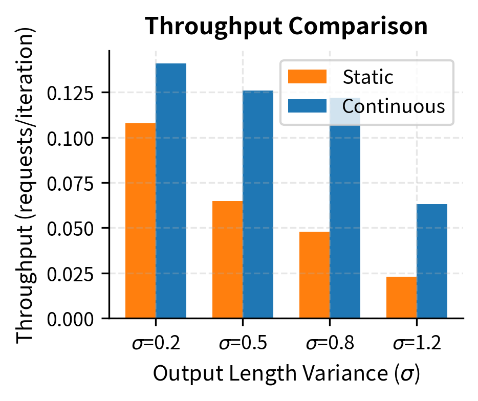
Let's run a more comprehensive simulation comparing the two approaches across a realistic workload. Theory tells us continuous batching should win, but simulation reveals the magnitude of improvement and how it varies with workload characteristics.
Continuous batching achieves significantly higher throughput and lower average latency. While the static batch is held back by the longest sequence in each group, continuous batching processes requests at their natural speed, returning short responses quickly while long ones continue processing.
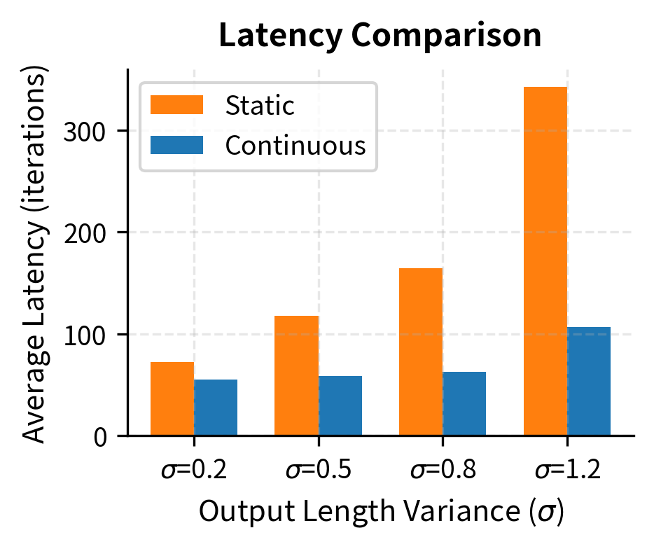
The improvement from continuous batching grows with output length variance. When all requests generate similar lengths, static batching loses less to waiting because the maximum is close to the average. But real workloads have high variance. Some of you ask for single-sentence summaries while others request long documents, making continuous batching essential for practical deployment.
Implementation Considerations
Building a production continuous batching system requires careful attention to several practical concerns that go beyond the basic algorithm. The theory is elegant, but the engineering details determine whether the system achieves its theoretical potential.
Memory Management Integration
Continuous batching works best when paired with paged attention, as covered in the Paged Attention chapter. Without it, memory fragmentation limits how many requests can be active simultaneously. Traditional contiguous allocation reserves maximum-length KV cache space for each request, even if most requests use far less. Paged attention allocates memory in small blocks on demand, enabling much higher concurrency.
Handling Preemption
When memory pressure is high, the scheduler might need to preempt active requests to make room for higher-priority work. This involves saving the request's state, including the KV cache and generated tokens, for later resumption. Preemption is a powerful tool for managing resources but adds significant complexity.
The decision of which request to preempt involves tradeoffs between fairness, throughput, and implementation complexity. Preempting a request that has generated many tokens wastes the computation invested in it. Preempting a request that has been preempted before may seem unfair. Different policies balance these concerns differently.
Batched Token Operations
For efficiency, token generation for all active requests should happen in a single batched forward pass. This requires careful tensor management to handle requests at different sequence positions. Unlike training, where all sequences in a batch are padded to the same length, continuous batching must handle sequences of varying lengths efficiently.
The key challenge is that different requests have different position embeddings and attention masks. Position embeddings tell the model where each token sits in its sequence. Attention masks prevent tokens from attending to future positions. Both vary by request, but both must be batched together for efficient GPU utilization.
The key insight is that despite requests being at different points in their generation, they can share a single forward pass because attention masks and position embeddings handle the differences. The input is just one token per request, but each token gets its own position embedding corresponding to its place in that request's sequence.
Key Parameters
The key parameters for the continuous batching implementation are:
- max_batch_size. Maximum number of concurrent requests. Higher values improve throughput but require more memory. The optimal value depends on model size, available GPU memory, and expected request characteristics.
- block_size. Number of tokens per memory block in paged attention. Typically 16 or 32. Smaller blocks reduce fragmentation but increase bookkeeping overhead.
- chunk_size. Number of tokens processed per iteration during prefill. Helps balance latency and throughput. Smaller chunks provide more responsive decode but may reduce prefill efficiency.
Real-World Performance
Production continuous batching systems like vLLM, TensorRT-LLM, and Text Generation Inference report significant improvements over static batching. These systems combine continuous batching with paged attention, optimized kernels, and sophisticated scheduling to achieve impressive throughput on commodity hardware.
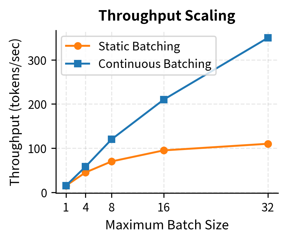
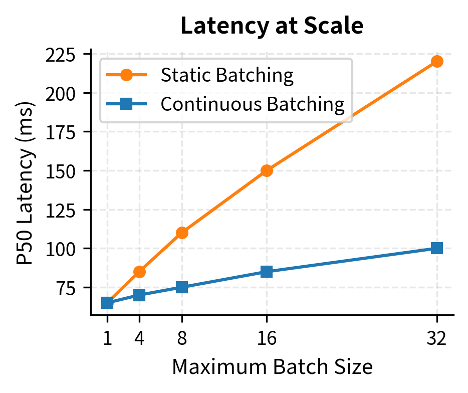
The throughput advantage of continuous batching compounds at larger batch sizes because GPU utilization stays high even as requests complete at different times. Static batching's throughput plateaus as the "waiting for slowest" overhead dominates, while continuous batching continues to scale.
Limitations and Impact
Continuous batching, while transformative for LLM serving, comes with its own set of challenges and tradeoffs that practitioners must understand. No optimization is free, and the benefits of continuous batching come with real engineering costs.
The primary complexity lies in implementation. A continuous batching system requires tight integration between the scheduler, memory manager, and model execution engine. The scheduler must make split-second decisions about which requests to run, potentially thousands of times per second. Any inefficiency in this hot path directly reduces throughput. Furthermore, debugging becomes harder when requests can be preempted, resumed, and interleaved in complex patterns. Reproducing issues requires capturing the exact sequence of scheduling decisions, which may be difficult in a highly dynamic system.
Memory management presents another significant challenge. While paged attention solves fragmentation, the combination of variable-length requests and preemption creates complex allocation patterns. Memory pressure can cascade: preempting one request to admit another might itself require preemption of a third request, leading to difficult-to-predict behavior. Production systems need careful tuning of admission policies and preemption thresholds to avoid thrashing.
There are also fairness considerations. Without careful policy design, long requests might be repeatedly preempted in favor of short ones, leading to starvation. Conversely, prioritizing completion of long requests might inflate latency for short queries. Finding the right balance depends on the specific application's requirements and your expectations.
Despite these challenges, continuous batching has fundamentally changed LLM deployment economics. Systems that previously needed multiple GPUs to serve moderate traffic can now handle the same load on a single device. This efficiency improvement makes LLMs practical for a much wider range of applications and organizations. The technique has become standard in production serving frameworks, and understanding its principles is essential for when you deploy language models at scale.
As we'll explore in the next chapter on Inference Serving, continuous batching is just one component of a complete serving system. Real deployments must also handle request routing, load balancing, model replication, and failure recovery, all while maintaining the low latency you expect.
Summary
Continuous batching transforms LLM inference from rigid, inefficient batch processing into a dynamic, high-utilization system. The key ideas we covered include:
- Static batching inefficiency. Traditional batching forces all requests to wait for the slowest, wasting compute on completed requests and inflating latencies
- Iteration-level scheduling. Treating each decode step as a scheduling opportunity allows immediate eviction of completed requests and admission of waiting ones
- Phase handling. Managing the distinct prefill and decode phases, potentially with chunked prefill, balances compute characteristics across the batch
- Resource management. Tight integration with KV cache memory management, including paged attention, maximizes the number of concurrent requests
- Throughput gains. Real-world improvements of 2-3x throughput are common, with better latency characteristics especially for short requests
Continuous batching is now standard practice for production LLM serving. Combined with the memory optimizations from paged attention and the speculative decoding techniques we covered earlier, it enables serving LLMs at scale with reasonable hardware costs.
Quiz
Ready to test your understanding? Take this quick quiz to reinforce what you've learned about continuous batching.

Comments