Speculative Decoding: Fast LLM Inference Without Quality Loss

Autoregressive generation, as we covered in Part XVIII, produces text one token at a time. Each forward pass through a large language model generates a single token, which then becomes input for the next pass. For a 70-billion parameter model generating a 500-token response, this means 500 sequential forward passes through the entire network. The process is slow, not because the GPU lacks computational power, but because it spends most of its time waiting for model weights to load from memory. This fundamental bottleneck has motivated you to find clever ways to extract more tokens from each expensive forward pass through the large model.

Speculative decoding attacks this problem with a clever insight: what if we could generate multiple tokens per forward pass of the large model? The approach uses a small, fast draft model to speculatively generate several candidate tokens, then verifies them all at once with the large target model. When the draft model's guesses align with what the target model would have produced, we get multiple tokens for the cost of one large-model forward pass. This technique can deliver 2-3x speedups without any approximation or quality loss. The target model's output distribution remains exactly preserved, meaning the text you generate is statistically indistinguishable from what you would have produced through standard autoregressive generation.

To understand why speculative decoding works, we need to understand why autoregressive generation is slow. Modern GPUs have enormous computational throughput. An NVIDIA A100 can perform 312 trillion floating-point operations per second. Yet generating tokens with a large language model barely scratches this capacity. The bottleneck isn't computation: it's memory bandwidth. Understanding this distinction is crucial because it reveals that the solution to slow inference isn't more computational power, but rather smarter use of the data movement that dominates generation time.

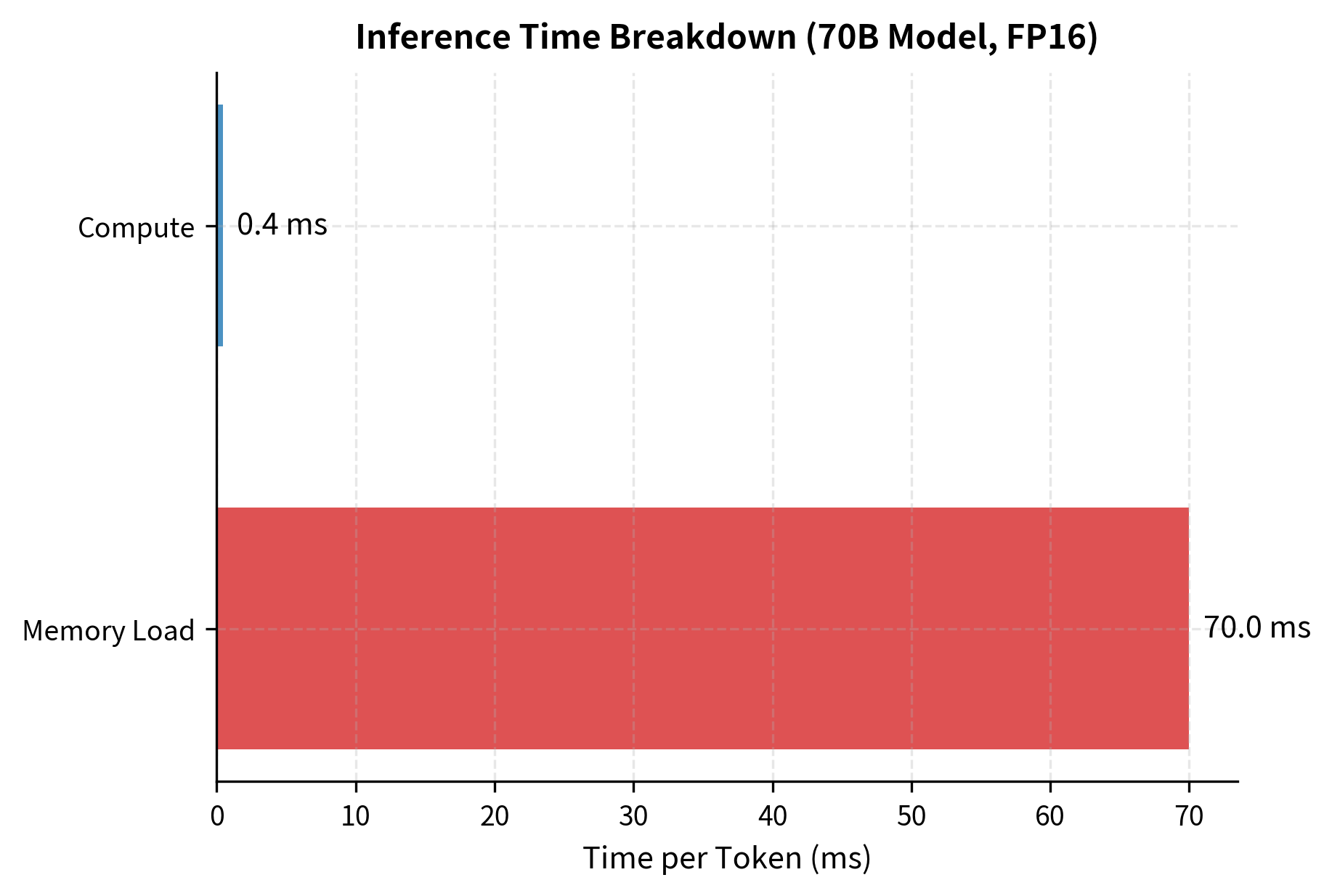
During inference, the GPU must load every model weight from memory for each forward pass. A 70B parameter model in 16-bit precision requires loading 140 GB of data per token generated. The A100's memory bandwidth of 2 TB/s means this takes roughly 70 milliseconds, during which the actual matrix multiplications complete almost instantly. The GPU spends over 95% of its time waiting for data transfer. This massive imbalance between data movement and computation is the key insight that speculative decoding exploits.

This phenomenon is captured by the arithmetic intensity metric, which measures the ratio of floating-point operations to bytes transferred. Training has high arithmetic intensity because gradients and activations reuse the same weights many times across large batch sizes. Inference has low arithmetic intensity because each token requires loading all weights for minimal computation. We say inference is memory-bound rather than compute-bound. This distinction is critical because memory-bound workloads cannot be sped up by adding more computational units; they can only be accelerated by reducing memory transfers or amortizing them across more useful work.

The arithmetic intensity of 1 FLOP per byte is far below the GPU's operational intensity (ratio of compute to bandwidth), which exceeds 150 FLOPs per byte for the A100. This confirms that inference is deeply memory-bound. We're moving data constantly but barely computing anything with it. The GPU's computational cores sit idle most of the time, waiting for the next batch of weights to arrive from memory.

The key insight for speculative decoding emerges from this analysis: if we process multiple tokens simultaneously, we can amortize the memory loading cost. Loading the model weights once and processing 5 tokens takes nearly the same time as processing 1 token, but produces 5x the output. The challenge is that autoregressive generation seems inherently sequential, since each token depends on all previous tokens. Speculative decoding overcomes this apparent limitation through a clever draft-and-verify strategy that preserves sequential correctness while enabling parallel verification.

Speculative decoding exploits this observation through a two-model architecture. A small, fast draft model generates multiple candidate tokens. The large target model then verifies all candidates in a single forward pass. If the draft model's predictions match what the target would have produced, we keep them. If they diverge, we reject the mismatched tokens and use the target model's correction. This approach transforms the problem from "how do we make the large model faster" to "how do we predict what the large model will say, so we can verify those predictions efficiently."

The process works in rounds. Each round proceeds as follows:

1. Draft phase: The draft model autoregressively generates $K$ candidate tokens (typically $K = 4$ to $8$)
2. Verify phase: The target model processes all $K$ candidates in one forward pass, computing the probability of each candidate given the preceding context
3. Accept/reject phase: Compare draft and target probabilities to decide which candidates to keep
4. Correction phase: If a candidate is rejected, sample a correction token from an adjusted distribution

The approach is simple: we make educated guesses about what the target model will say, then check those guesses efficiently. When our guesses are good (the draft model is well-aligned with the target), we save significant time. When our guesses are wrong, we still make progress by accepting the target model's correction.

The key efficiency gain comes from the verification phase. When we pass $K$ draft tokens to the target model, we leverage the parallelism of the transformer architecture. Computing attention over a sequence of $K$ additional tokens requires nearly the same memory bandwidth as computing attention for 1 token, since we load the model weights just once. The computational cost increases linearly with $K$, but as we established, the computational cost is negligible compared to memory transfer. This means that verifying 5 draft tokens costs almost the same wall-clock time as verifying 1 token, creating the opportunity for substantial speedups when draft tokens are accepted.

How does the target model verify multiple tokens in one forward pass? The answer lies in the causal attention mask we covered in Part X, Chapter 4. This mechanism, originally designed to enable efficient training on entire sequences, turns out to be exactly what we need for parallel verification during inference.

When we feed the sequence $[\text{prompt}, \text{draft}_1, \text{draft}_2, \text{draft}_3, \text{draft}_4]$ to the target model, the causal mask ensures each position only attends to preceding tokens. This creates a natural structure where each position independently computes the probability of its token given everything that came before.

At position $\text{draft}_1$, the model computes $p(\text{draft}_1 | \text{prompt})$. At position $\text{draft}_2$, it computes $p(\text{draft}_2 | \text{prompt}, \text{draft}_1)$. Each position's output gives us the probability the target model assigns to the draft token at that position, conditioned on everything before it. Crucially, these computations happen simultaneously in a single forward pass, not sequentially as they would in standard autoregressive generation.

This parallel verification is what makes speculative decoding efficient. Without it, verifying $K$ tokens would require $K$ forward passes through the target model, eliminating any speedup. With it, we amortize the memory bandwidth cost across $K$ potential tokens. The causal mask ensures that even though we process all positions simultaneously, each position's output depends only on previous positions, maintaining the autoregressive property that makes language model outputs coherent and consistent.

The choice of draft model critically affects speculative decoding performance. A good draft model balances three competing requirements: speed, alignment with the target model, and vocabulary compatibility. Getting this balance right is often the most challenging aspect of deploying speculative decoding in practice.

The draft model must be fast enough that generating $K$ tokens takes less time than one target model forward pass. If the draft model is too slow, the combined draft-plus-verify time exceeds standard autoregressive generation, producing a slowdown rather than speedup. This constraint places an upper bound on draft model size, typically limiting it to 10-15% of the target model's parameters.

Consider a target model requiring 100ms per forward pass. If we draft $K=5$ tokens and each draft forward pass takes 15ms, drafting costs 75ms. Total round time is 175ms. For this to beat standard generation, we need to accept more than 1.75 tokens per round on average, since standard generation takes 100ms per token. This threshold determines whether speculative decoding provides a net benefit or a net loss.

The table reveals a crucial insight: acceptance rate dramatically affects speedup. At 90% acceptance, we achieve 2.6x speedup. At 50% acceptance, speedup drops to 1.2x. This makes draft model alignment the dominant factor in speculative decoding performance. The time invested in finding or training a well-aligned draft model pays dividends throughout the system's deployment lifetime.

A draft model is well-aligned when its probability distribution closely matches the target model's. If the draft model assigns high probability to the same tokens the target model prefers, acceptance rates will be high. If they diverge significantly, most draft tokens will be rejected. This alignment is measured empirically by running both models on the same inputs and comparing their probability distributions.

Common approaches to obtaining aligned draft models include:

• Distillation: Train a small model specifically to match the target model's output distribution. This creates the best alignment but requires training infrastructure.
• Model families: Use a smaller model from the same family (e.g., LLaMA-7B drafting for LLaMA-70B). Same training data and architecture often lead to aligned predictions.
• Same-model layers: Use early exit from the target model itself, treating the first N layers as a draft model.

The model family approach is most practical for deployment. LLaMA-2-7B achieves approximately 70-80% acceptance rates when drafting for LLaMA-2-70B on typical text. Distilled models can achieve 85%+ acceptance rates. The choice between these approaches depends on the available resources and the importance of maximizing speedup.

The draft and target models must share exactly the same vocabulary and tokenizer. If they tokenize text differently, the draft tokens cannot be verified by the target model, because the token IDs would refer to different subwords. This requirement has significant practical implications.

This requirement constrains draft model selection significantly. You cannot use a GPT-2 draft model with a LLaMA target model, even if they might produce similar text. The tokens simply don't correspond. This constraint means that speculative decoding works best within model families that share tokenizers, and organizations often need to train custom draft models when working with proprietary target models that use unique tokenization schemes.

The verification procedure determines which draft tokens to accept and how to correct rejections. We can construct an acceptance criterion that exactly preserves the target model's output distribution while maximizing the number of accepted tokens. This is not an approximation or heuristic; it is a mathematically guaranteed property that makes speculative decoding a lossless acceleration technique.

For each draft token, we compare the draft model's probability $q(x)$ with the target model's probability $p(x)$. The acceptance probability is:

where:

• $\alpha(x)$: the probability of accepting candidate token $x$
• $p(x)$: the probability assigned to token $x$ by the target model
• $q(x)$: the probability assigned to token $x$ by the draft model
• $1$: the upper bound, ensuring probability never exceeds certainty

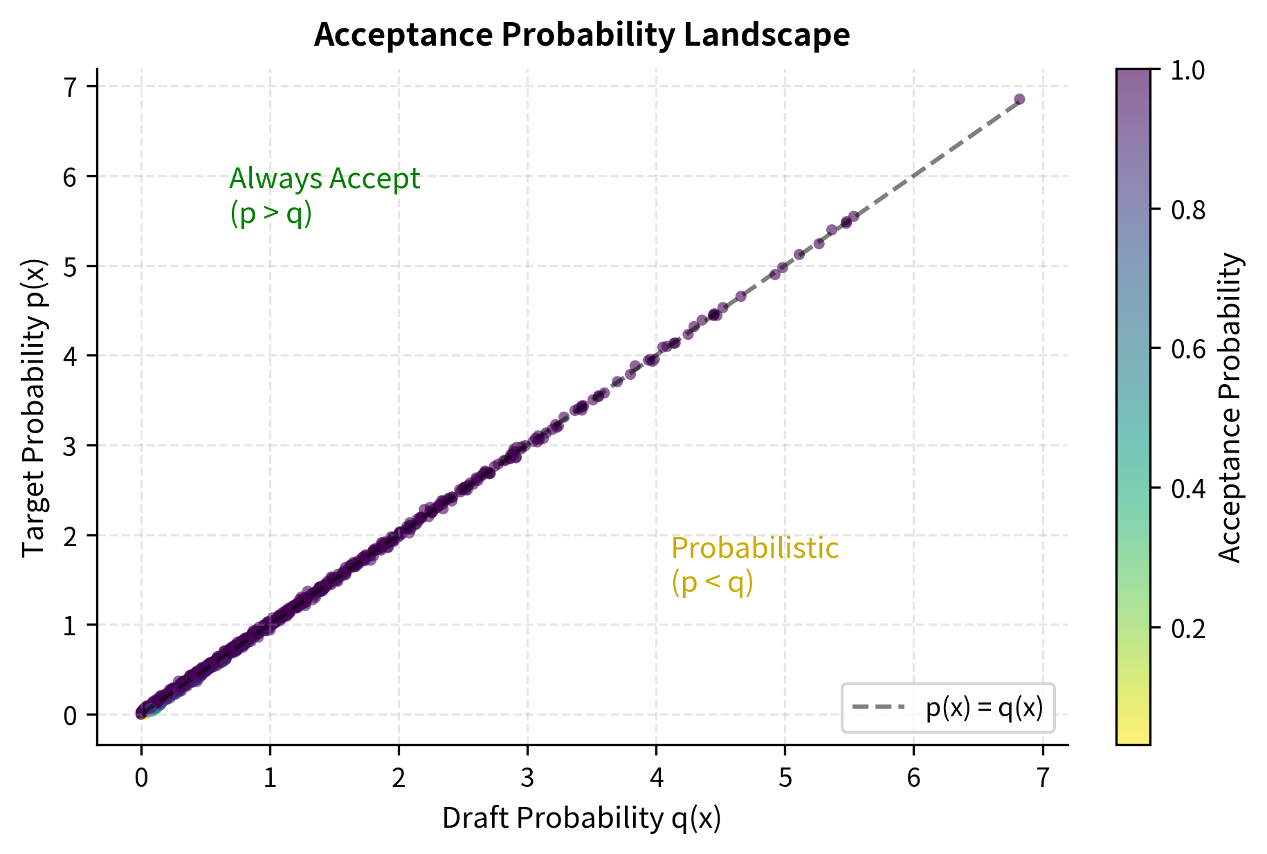
This formula has an elegant interpretation. When $p(x) \geq q(x)$ (the target model likes this token as much or more than the draft model), we always accept. This makes sense because the target model considers this token at least as likely as the draft model did, so accepting it aligns with the target's preferences. When $p(x) < q(x)$ (the draft model overestimated this token's likelihood), we accept with probability proportional to how much it overestimated. The more the draft model overestimated, the lower our acceptance probability, ensuring we don't bias our output toward tokens the draft model unfairly favored.

The results show that we accept with certainty when the target model prefers a token (Probability 1.00), but only probabilistically when the draft model is overconfident. This mechanism ensures the accepted tokens strictly follow the target distribution. The mathematical proof of this property, which we will cover in the next chapter, shows that the combination of this acceptance criterion with the correction distribution produces samples that are exactly distributed according to the target model.

When a draft token is rejected, we need to sample a correction token. Simply sampling from the target model's distribution would bias the output: we would undersample tokens that were already accepted and oversample tokens that were never drafted. The correction distribution must account for the tokens that would have been accepted under the draft-then-accept procedure.

The correction distribution adjusts for the tokens that would have been accepted:

where:

• $p_{\text{correction}}(x)$: the adjusted probability of sampling token $x$ as a correction
• $p(x) - q(x)$: the difference between target and draft probabilities
• $\max(0, \dots)$: filter ensuring we only consider under-sampled tokens (where target > draft)
• $\sum_{x'} \dots$: the normalization constant computed over the entire vocabulary

This distribution has an intuitive interpretation. It samples only from tokens where the target model assigns more probability than the draft model. These are precisely the tokens that were "under-represented" by the draft model's proposal. By sampling from this residual distribution, we fill in the probability mass that was "missed" by the draft model, ensuring that the overall output distribution matches the target exactly.

Notice how the correction distribution emphasizes token 0 and token 2, where the target model assigns more probability than the draft. Token 1 and token 3 receive zero correction probability because the draft model already over-sampled them. This selective correction ensures that when we combine the accepted draft tokens with the correction samples, the overall distribution perfectly matches what the target model would have produced through standard autoregressive generation.

During verification, we process draft tokens sequentially and stop at the first rejection. If draft token 3 is rejected, we don't verify tokens 4 and beyond. This is because the correction at position 3 changes the context, invalidating the draft model's predictions for subsequent positions. The draft model generated tokens 4 and beyond assuming token 3 would be accepted, so once we substitute a different correction token, those subsequent predictions become meaningless.

This sequential processing means expected accepted tokens follow a geometric-like distribution. With acceptance rate $\gamma$ per token, the expected total number of tokens generated per round is:

where:

• $\mathbb{E}[\text{tokens}]$: the expected number of tokens produced (drafts + correction)
• $1$: the correction token, which is always generated
• $\sum_{k=1}^{K} \gamma^k$: the expected number of accepted draft tokens
• $\gamma$: the probability of accepting a single draft token
• $K$: the number of draft tokens attempted

This formula sums the always-present correction token with the geometric series of accepted drafts. The geometric series arises because each subsequent draft token can only be accepted if all previous draft tokens were also accepted. The probability of accepting the first two drafts is $\gamma^2$, the first three is $\gamma^3$, and so on. This cumulative structure explains why acceptance rate has such a dramatic effect on speedup, as small improvements in $\gamma$ compound across multiple positions.

The acceptance rate $\gamma$ is the probability that a given draft token is accepted. It depends on how well the draft model's distribution matches the target model's. This metric captures draft model quality and determines whether speculative decoding will provide meaningful speedups.

Empirical acceptance rate is measured by running speculative decoding on representative text and tracking the fraction of draft tokens accepted:

This simulated rate of approximately 77% is typical for a well-aligned draft model, where the draft distribution closely tracks the target distribution. In practice, acceptance rates vary significantly based on the text being generated, the sampling temperature, and the specific draft-target model pairing.

Several factors influence acceptance rate in practice, and understanding these factors helps you optimize your speculative decoding deployments:

Model family similarity: Draft models from the same family as the target (e.g., LLaMA-7B for LLaMA-70B) typically achieve 70-85% acceptance rates. Models from different families may drop to 40-60%. This improvement comes from shared training data, similar architectures, and aligned tokenization schemes that cause both models to "think" in similar ways about the same inputs.

Temperature: Higher sampling temperatures increase randomness, generally reducing acceptance rates. At temperature 0 (greedy decoding), acceptance is deterministic based on whether draft and target agree on the argmax. As temperature increases, both models become less confident, and their probability distributions flatten, making disagreements more likely even when they agree on the most likely tokens.

Context type: Acceptance rates vary by content. Factual text with predictable continuations achieves higher acceptance than creative writing or code with many valid alternatives. When there is a clear "right answer" that both models recognize, acceptance is high. When multiple reasonable continuations exist, the models may prefer different alternatives, lowering acceptance.

Sequence position: Early tokens in a response may have lower acceptance as the models "warm up" to the context. Later tokens often show higher acceptance once both models have established similar interpretations. This pattern suggests that the models' internal representations converge as they process more context together.

As temperature increases, the distributions flatten and diverge, causing the acceptance rate to drop significantly. This highlights why speculative decoding is most effective for lower-temperature, more deterministic generation tasks. For applications like creative writing that benefit from higher temperatures, the speedup from speculative decoding will be more modest.

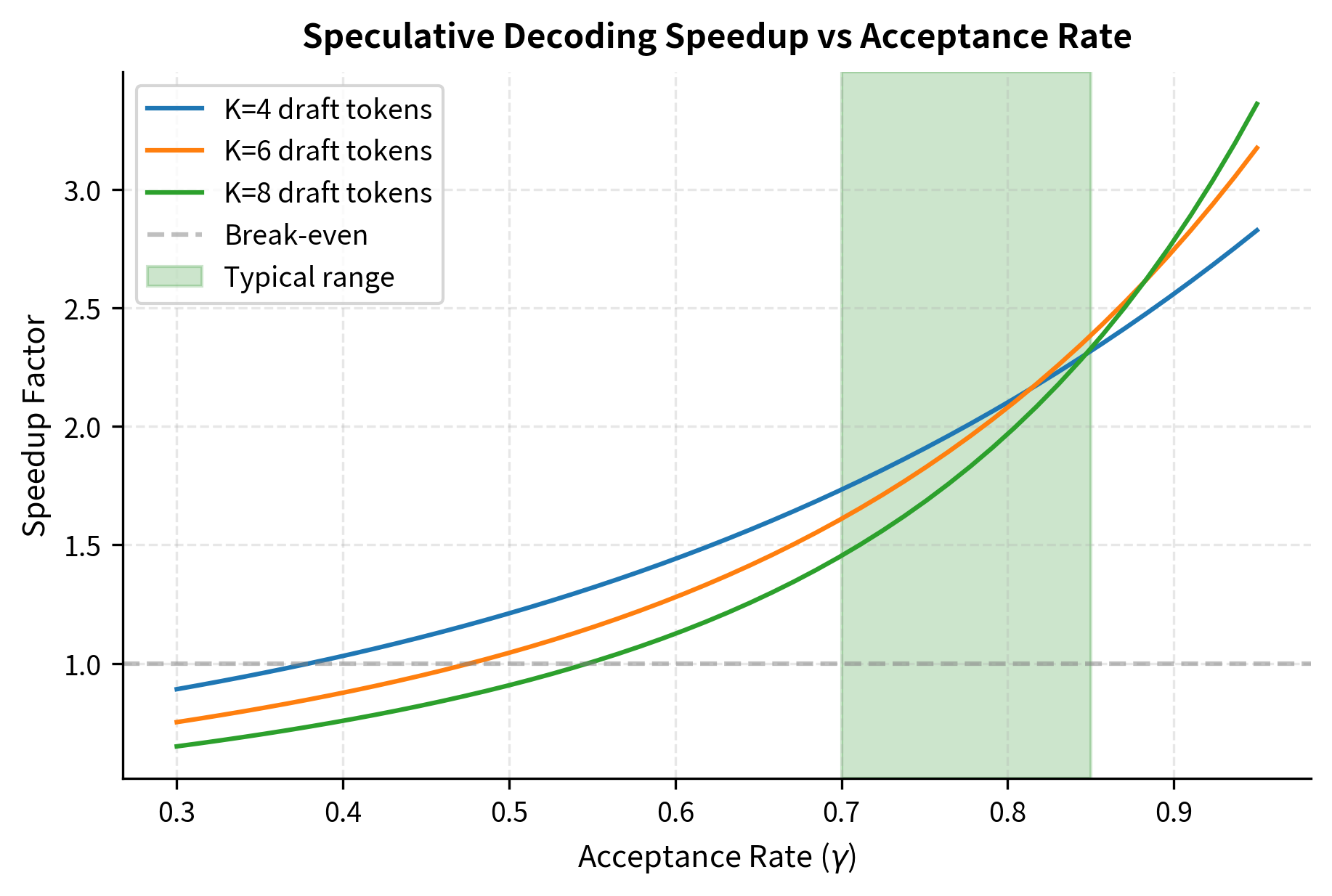
The relationship between acceptance rate and speedup is highly nonlinear. Small improvements in acceptance rate yield disproportionate speedup gains because more consecutive tokens pass verification. This nonlinearity arises from the geometric nature of sequential acceptance: improving acceptance from 70% to 80% doesn't just improve each token's acceptance by 10%, it dramatically increases the probability of long acceptance runs.

The plot demonstrates the importance of draft model alignment. Moving from 70% to 85% acceptance rate approximately doubles the speedup. This nonlinear relationship motivates significant investment in draft model quality. Even modest improvements in alignment can translate to substantial real-world performance gains, making draft model optimization a high-leverage activity for production deployments.

This section presents a complete speculative decoding implementation using the Hugging Face transformers library. We'll use actual models to demonstrate the concept with measurable results. This implementation captures all the key components we've discussed: draft generation, parallel verification, and the acceptance/correction procedure.

For demonstration, we'll use small models that can run on limited hardware. The concepts apply identically to larger production models. The key requirement is that both models share the same vocabulary, which GPT-2 and GPT-2-medium naturally satisfy since they use the same tokenizer.

The core implementation encapsulates the three main operations: drafting candidate tokens, verifying them against the target model, and applying the acceptance/rejection logic. Each method is designed to be modular and easy to understand.

This function orchestrates the complete generation process, repeatedly running speculative decoding rounds until we've generated the desired number of tokens. It also tracks statistics that help us understand the system's performance.

To measure the benefit of speculative decoding, we need a baseline. This standard autoregressive generation function provides that baseline, using the same target model but generating one token at a time.

Since loading actual models requires significant resources, we demonstrate the workflow with a simulation that captures the key dynamics. This simulation explores how different acceptance rates affect performance without requiring large language models.

The simulation confirms our theoretical analysis. At 80% acceptance rate, we achieve approximately 2x speedup, generating over 3 tokens per round on average. This matches well with reported results from production speculative decoding systems, validating that our theoretical framework accurately predicts real-world performance.

The key parameters for Speculative Decoding are:

• draft_model: The smaller, faster model used to generate candidate tokens.
• target_model: The larger model used to verify candidates and guarantee output distribution.
• acceptance_rate ($\gamma$): The probability that a draft token matches the target model's preference.
• num_draft_tokens ($K$): The number of candidate tokens generated per round. Typically 4-8.
• temperature: Controls randomness. Higher temperature usually reduces acceptance rate.

Speculative decoding offers compelling speedups but comes with important limitations that affect deployment decisions. Understanding these tradeoffs helps you decide when and how to apply the technique.

The most significant constraint is the requirement for a well-aligned draft model. Finding or training a draft model that achieves 70%+ acceptance rate while being fast enough to provide speedups is non-trivial. For proprietary models without available smaller variants, this can be a blocking issue. Some organizations train dedicated draft models using distillation, but this adds significant infrastructure overhead and requires access to the target model's output distribution during training. The alternative of using early layers of the target model (self-speculative decoding) avoids this problem but requires architectural modifications.

Memory requirements increase because both models must be loaded simultaneously. For a 70B target model with a 7B draft model, total memory increases by roughly 10%. On memory-constrained deployments, this overhead may prevent using speculative decoding entirely or force quantization of one or both models. The interaction between quantization (covered in Chapters 5-9 of this part) and speculative decoding remains an active research area: quantizing the draft model more aggressively than the target model can preserve quality while minimizing the memory overhead.

Batched inference presents complications that can negate speculative decoding benefits. When serving multiple concurrent requests, the sequences in a batch may have different acceptance patterns. One sequence might accept all 5 draft tokens while another rejects after 2. Handling this efficiently requires sophisticated orchestration, which we'll explore in the upcoming chapter on Continuous Batching. The simpler approach of running speculative decoding independently per sequence underutilizes batch parallelism.

Despite these limitations, speculative decoding has become a standard technique in production LLM serving. The 2-3x speedups it provides translate directly to reduced latency for you and reduced cost for providers. For conversational applications where response time critically affects user experience, shaving 50-70% off generation time is transformative.

The technique also demonstrates a broader principle: the memory-bound nature of LLM inference creates opportunities for clever algorithmic improvements that don't require hardware upgrades or model changes. Speculative decoding preserves the exact output distribution of the target model while improving efficiency, a rare win-win in machine learning optimization.

Looking ahead, the mathematical foundations of speculative decoding that guarantee distribution preservation are covered in the next chapter. Understanding these proofs explains why the acceptance criterion takes the form it does and enables extensions like tree-structured speculation where multiple draft paths are explored simultaneously.

Speculative decoding accelerates autoregressive generation by parallelizing token verification. A small draft model generates multiple candidate tokens, which the large target model verifies in a single forward pass. The technique exploits the memory-bound nature of LLM inference, where processing multiple tokens costs nearly the same as processing one.

The key components form an interconnected system: the draft model must be fast and well-aligned with the target, the acceptance criterion must preserve the target distribution, and the correction distribution must compensate for rejected tokens. The acceptance rate emerges as the critical metric, with small improvements yielding disproportionate speedup gains due to the geometric accumulation of consecutive acceptances.

Draft model selection balances speed against alignment quality. Model family relationships provide the most practical path, with smaller models from the same training pipeline achieving 70-80% acceptance rates. Distilled models can push this higher at the cost of training infrastructure.

The verification procedure guarantees that speculative decoding produces exactly the same output distribution as standard autoregressive generation from the target model. This mathematical guarantee, which we'll prove in the next chapter, makes speculative decoding a lossless acceleration technique: improving efficiency without compromising quality.

Ready to test your understanding? Take this quick quiz to reinforce what you've learned about speculative decoding.