

Master LLM inference serving architecture, token-aware load balancing, and auto-scaling. Optimize time-to-first-token and throughput for production systems.

This article is part of the free-to-read Language AI Handbook
Choose your expertise level to adjust how many terms are explained. Beginners see more tooltips, experts see fewer to maintain reading flow. Hover over underlined terms for instant definitions.
Inference Serving
Deploying a language model involves much more than loading weights and running forward passes. Production systems must handle thousands of concurrent users, maintain low latency under varying load, and do so cost-effectively. Inference serving encompasses the architecture, routing, and scaling strategies that transform a trained model into a reliable, performant service.
The previous chapters in this part covered techniques that make individual inference requests faster and more memory-efficient: KV caching reduces redundant computation, quantization shrinks memory footprints, speculative decoding accelerates token generation, and continuous batching maximizes GPU utilization. This chapter focuses on the layer above: how to orchestrate these capabilities into a production system that serves many users simultaneously while meeting latency and throughput requirements.
Inference Server Architecture
An inference server sits between client applications and the underlying model, handling request management, batching, scheduling, and response streaming. Modern LLM inference servers have evolved specialized architectures to address the unique challenges of autoregressive generation. Understanding these architectural patterns is essential for anyone building or operating production language model services.
Core Components
The architecture of an LLM inference server differs significantly from traditional ML serving systems in fundamental ways that stem from the nature of autoregressive text generation. Classification models process requests independently with fixed compute costs: an image classifier performs the same computation regardless of the input image's content. Language models, by contrast, generate tokens iteratively, with each request potentially requiring hundreds of forward passes and memory that grows with sequence length. This iterative, variable-cost nature demands specialized architectural components that can efficiently manage the unique resource patterns of text generation.
A typical inference server contains several interconnected components, each playing a distinct role in the request processing pipeline:
-
Request handler: Accepts incoming requests over HTTP/gRPC, validates inputs, and manages response streaming. For LLMs, this often involves Server-Sent Events (SSE) or WebSocket connections to stream tokens as they're generated. The request handler must maintain long-lived connections efficiently, as a single request may take several seconds to complete while tokens are progressively returned to the client.
-
Tokenizer: Converts text to token IDs on input and back to text on output. While fast compared to model inference, tokenization can become a bottleneck at high throughput because it runs on the CPU while the model runs on the GPU. Servers often parallelize tokenization across CPU cores to prevent this component from limiting overall system throughput.
-
Scheduler: Determines which requests to process together in each batch. As we discussed in the previous chapter on continuous batching, sophisticated schedulers dynamically add and remove requests from running batches. The scheduler must balance multiple objectives: maximizing GPU utilization, maintaining fair request ordering, and meeting latency targets for high-priority requests.
-
Model executor: Manages the actual model inference, including memory allocation for KV caches, attention computation, and integration with optimized kernels like FlashAttention. This component coordinates the GPU computation and ensures that the model weights, activations, and cached attention states are efficiently arranged in memory.
-
Memory manager: Tracks KV cache allocations, implements paged attention for efficient memory use, and handles memory pressure through eviction policies. Because KV cache memory requirements grow with sequence length and concurrent request count, intelligent memory management is critical for maintaining high throughput without running out of GPU memory.
Popular Inference Frameworks
Several frameworks have emerged to handle LLM serving at scale, each with different strengths and design philosophies:
vLLM implements PagedAttention for efficient KV cache management, enabling high throughput with memory-constrained hardware. By treating KV cache memory like virtual memory pages, vLLM can handle more concurrent requests than naive implementations that allocate contiguous memory blocks. It supports continuous batching and integrates with popular model architectures, making it a popular choice for production deployments.
Text Generation Inference (TGI) from Hugging Face provides production-ready serving with tensor parallelism for multi-GPU deployments, quantization support, and optimized attention implementations. Its tight integration with the Hugging Face ecosystem makes it particularly convenient for teams already using Transformers for model development.
TensorRT-LLM from NVIDIA offers highly optimized inference for NVIDIA GPUs, with custom CUDA kernels and support for quantization schemes like FP8 and INT4. When running on NVIDIA hardware, TensorRT-LLM often achieves the highest raw performance, though it requires more effort to set up than framework-agnostic alternatives.
Triton Inference Server provides a model-agnostic serving platform that can host multiple models with different backends, useful for ensemble architectures or multi-model deployments. Its flexibility makes it well-suited for complex inference pipelines that combine multiple models or processing steps.
The configuration balances memory allocation against concurrency in a careful trade-off. Higher gpu_memory_utilization allows more KV cache space for concurrent requests, but leaves less headroom for activation memory during computation. Setting this value too high can cause out-of-memory errors during prefill of long sequences; setting it too low wastes expensive GPU memory that could support additional concurrent requests.
Key Parameters
The key parameters for inference server configuration are:
- gpu_memory_utilization: Fraction of GPU memory to reserve for the model weights and KV cache.
- max_num_seqs: Maximum number of concurrent sequences the server can handle.
- enable_chunked_prefill: Whether to split the prefill phase into chunks to prevent blocking the decode phase of other requests.
Request Lifecycle
Understanding the journey of a request through the server helps identify optimization opportunities and debug performance issues. Each stage presents different bottlenecks and optimization levers:
-
Arrival: The request arrives via HTTP POST with prompt text and generation parameters (temperature, max tokens, etc.). The server validates the request format and assigns it a unique identifier for tracking.
-
Preprocessing: The server tokenizes the prompt and validates that the resulting sequence fits within model limits. Long prompts may be rejected or truncated depending on server configuration.
-
Scheduling: The scheduler decides when to begin processing. The request may queue if all batch slots are occupied. Priority and fairness policies determine ordering among waiting requests.
-
Prefill: The model processes all prompt tokens in parallel, populating the KV cache with attention states for all input positions. This phase is compute-bound because it performs dense matrix multiplications across the entire prompt length.
-
Decode Loop: Tokens are generated one at a time, with each new token streamed to the client. This phase is memory-bandwidth-bound because each forward pass must read the entire KV cache from GPU memory while producing only a single output token.
-
Completion: Generation stops when the model produces an end token or reaches the maximum length. The server releases KV cache memory and closes the response stream, making capacity available for new requests.
The metrics distinguish between time-to-first-token (TTFT) and total latency because these capture fundamentally different aspects of user experience. TTFT measures user-perceived responsiveness in streaming applications: when you send a message, how quickly you see the model start to respond? Total latency matters more for batch processing where results are consumed only after complete generation. Optimizing these metrics often involves different trade-offs. For example, aggressive batching improves total throughput but can increase TTFT because requests wait for batch formation.
Request Routing
When multiple model instances serve requests, a routing layer decides which instance handles each request. Effective request routing maximizes throughput while maintaining consistent latency. The routing layer must make rapid decisions with incomplete information, balancing immediate load distribution against longer-term efficiency considerations.
Model Routing Strategies
Simple deployments route all requests to a single model version, treating the routing problem as pure load balancing. Production systems often need more sophisticated routing that considers request characteristics and business requirements:
Version-based routing directs requests to different model versions based on request metadata. This enables A/B testing by directing a fraction of traffic to a new model version, gradual rollouts that progressively shift traffic to updated models, and fallback to stable versions if new deployments exhibit problems. For example, a system might route 5% of traffic to a new model version while monitoring quality metrics before expanding the rollout.
Capability-based routing matches requests to appropriate models based on task complexity or domain. A lightweight model might handle simple queries like basic factual questions, while complex reasoning tasks route to larger, more capable models. This approach reduces cost without sacrificing quality where it matters: simple questions get fast, cheap answers while challenging problems receive appropriate computational resources.
Priority routing ensures high-priority requests (paying customers, critical applications) get preferential treatment in terms of both queue position and endpoint selection. Lower-priority requests may queue longer or route to less powerful instances. This enables tiered service levels without requiring completely separate infrastructure for each tier.
The router considers both capacity and priority when making routing decisions. High-priority requests route to the least-loaded endpoint to minimize queuing time and ensure fast response. Lower-priority requests distribute randomly among available endpoints to prevent creating hotspots while still avoiding overloaded instances. This differentiated treatment allows the system to provide better service to priority traffic without completely starving lower-priority requests.
Health Checks and Failover
Effective routing depends on accurate health information about each endpoint. If the router sends requests to an unhealthy endpoint, those requests will fail or experience long delays. Servers implement multiple health check levels to detect different kinds of problems:
-
Liveness checks verify the process is running and responding to basic probes. A hanging process fails liveness checks even if it hasn't technically crashed. These checks detect catastrophic failures quickly.
-
Readiness checks verify the server can accept new requests. A server in the process of loading a model passes liveness (the process is running) but fails readiness (it cannot yet serve requests). This distinction prevents routing traffic to instances that are starting up.
-
Deep health checks verify end-to-end functionality by running test inferences. These checks catch subtle issues like corrupted model weights, CUDA driver problems, or memory leaks that wouldn't be detected by simpler checks. The trade-off is that deep checks consume GPU resources and take longer to complete.
Health checks enable automatic failover without human intervention. When an endpoint exceeds the failure threshold (typically 3 consecutive failures), the router removes it from rotation and stops sending new requests. This prevents user-facing errors from accumulating while the underlying issue is investigated. After the underlying issue resolves, consecutive successful checks restore the endpoint to service. The recovery threshold ensures the endpoint is genuinely healthy before receiving traffic again, preventing oscillation between healthy and unhealthy states.
Load Balancing
Load balancing distributes requests across multiple model instances to maximize throughput and maintain consistent latency. While load balancing is a well-studied problem in distributed systems, LLM serving presents unique challenges that traditional load balancing algorithms don't address well. The variable cost of requests, the long-running nature of generation, and the importance of memory locality all complicate the problem.
Traditional Algorithms
Standard load balancing approaches provide a foundation for understanding the problem, even if they don't fully address LLM-specific challenges:
Round-robin distributes requests sequentially across endpoints in a fixed order. The first request goes to endpoint 0, the second to endpoint 1, and so on, cycling back to 0 after reaching the last endpoint. This approach is simple, predictable, and fair in terms of request count. However, it ignores actual load, which matters when requests have varying computational costs. A long generation request and a short one count equally, even though they impose vastly different burdens.
Least connections routes each new request to the endpoint with the fewest active requests. This approach adapts better to variable-duration requests because endpoints processing long requests naturally accumulate fewer connections over time. However, it still treats all requests as equal cost, which fails to capture the difference between generating 10 tokens and generating 1000 tokens.
Weighted distribution assigns requests proportionally to endpoint capacity, which is useful when endpoints have different hardware. An H100 GPU might receive twice as many requests as an A100 because it can process them twice as fast. Weights can be configured manually based on hardware specs or adjusted dynamically based on observed performance.
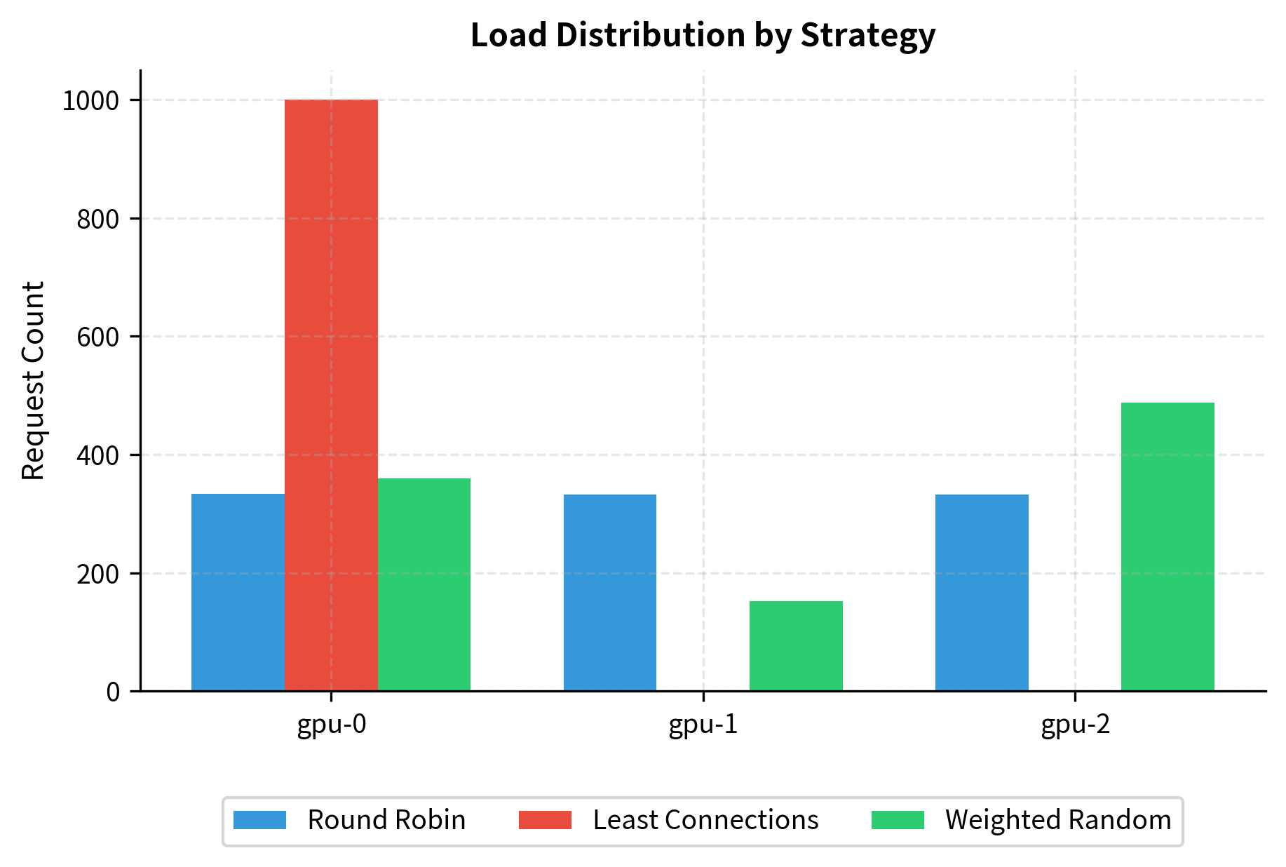
The results illustrate the behavioral differences between strategies. Round-robin distributes evenly regardless of load, giving each endpoint roughly 33% of requests. Least connections concentrates traffic on the least-loaded endpoint (gpu-0), which may improve its latency but could overload it if requests are long-running. Weighted random accounts for available capacity, directing more requests to endpoints with headroom while maintaining some randomness to avoid perfect synchronization effects.
Token-Aware Load Balancing
Traditional metrics like connection count fail to capture LLM workload characteristics because they treat all requests as having equal cost. In reality, a request generating 1000 tokens consumes far more GPU resources and time than one generating 10 tokens, even though both count as single connections. Similarly, a request with a 4000-token prompt requires substantially more prefill computation than one with a 100-token prompt.
Token-aware load balancing accounts for the actual computational cost of requests by tracking token counts rather than just request counts. This provides a much more accurate picture of actual endpoint load:
Token-aware balancing makes smarter routing decisions by considering the actual work each endpoint is performing. In this example, gpu-0 has more prompt tokens queued for prefill, but gpu-1 has more active decode tokens. Because decode is the bottleneck phase (each token requires reading the entire KV cache), the long-output request routes to gpu-0, which has less active decoding. This prevents one endpoint from becoming decode-saturated while another sits idle during its compute-bound prefill phase.
Session Affinity Considerations
Some applications benefit from routing subsequent requests to the same endpoint to enable optimization opportunities. If a conversation spans multiple API calls with the same system prompt or shared context, routing to the same instance enables KV cache reuse through prefix caching, as discussed earlier in this part. Rather than recomputing attention states for the repeated prefix, the server can reuse cached values, significantly accelerating prefill.
However, session affinity conflicts with optimal load balancing because it constrains routing decisions. If a particular session's preferred endpoint becomes overloaded, the system must choose between maintaining affinity (and accepting higher latency) or breaking affinity (and losing cache benefits). A simple compromise routes requests with known session IDs to consistent endpoints using hash-based assignment, while distributing new sessions based on current load:
Consistent hashing ensures the same session always reaches the same endpoint, assuming the endpoint pool remains stable. This deterministic mapping enables KV cache hits for repeated prompts within a conversation. When endpoints are added or removed, consistent hashing minimizes disruption by changing the mapping for only a fraction of sessions rather than all of them. More sophisticated approaches can combine affinity preferences with load awareness, preferring the affinity endpoint when it has capacity but falling back to other endpoints when necessary.
Auto-Scaling
Static deployments with a fixed number of instances struggle with variable demand. Traffic to inference services often varies dramatically by time of day, day of week, and in response to external events. Auto-scaling adjusts the number of model instances based on load, reducing costs during low-traffic periods while maintaining performance during peaks. This elastic capacity is one of the key advantages of cloud deployments over fixed on-premises infrastructure.
Scaling Metrics
Choosing the right metrics to trigger scaling is crucial because different metrics capture different aspects of system health and have different response characteristics. Common options for LLM serving include:
Queue depth: The number of waiting requests provides a direct measure of demand exceeding capacity. High queue depth indicates insufficient capacity and directly predicts increased latency for arriving requests. This metric responds quickly to load changes because queues grow immediately when arrivals exceed processing rate.
Latency percentiles: The P50, P95, or P99 request latency directly measures user experience. Scaling based on latency targets addresses user experience directly, which is ultimately what matters. However, latency increases only after the system is already overloaded, making this a lagging indicator. By the time latency rises, users have already experienced degraded service.
GPU utilization: The fraction of GPU compute being used indicates how efficiently the current capacity is being used. Low utilization suggests over-provisioning and wasted cost. Consistently high utilization suggests under-provisioning and risk of latency degradation as load increases further.
Tokens per second: The aggregate throughput across instances measures actual work being done. Unlike request count, this metric accounts for variable request sizes. A spike in tokens per second indicates increased load even if request count is stable (perhaps because users are submitting longer prompts).
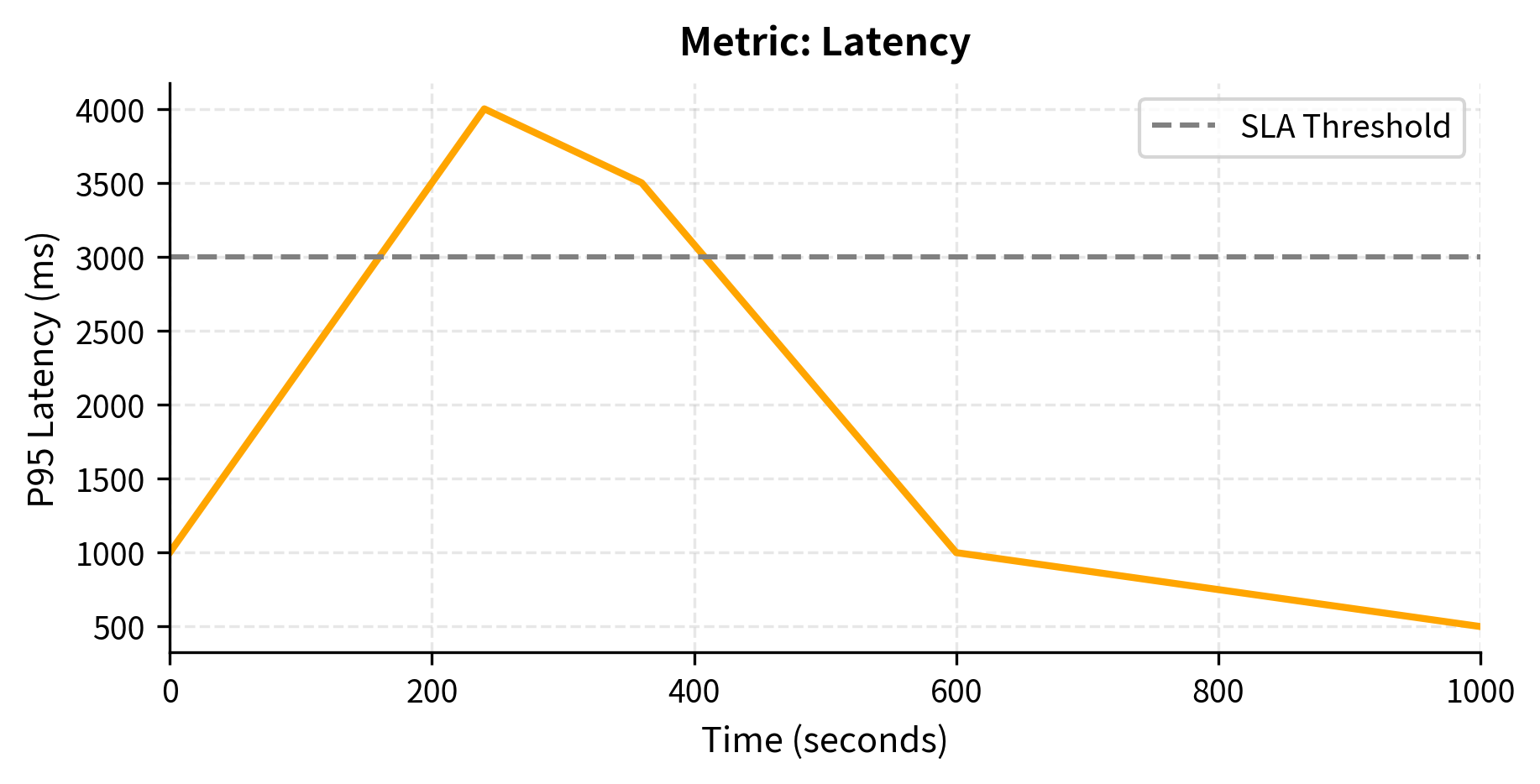
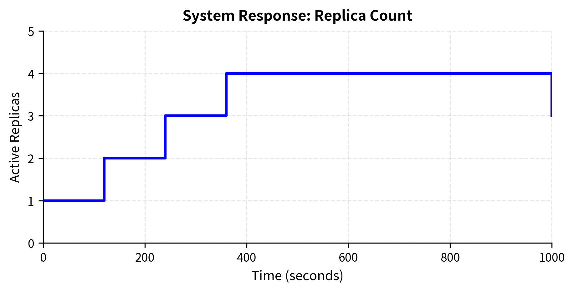
The simulation illustrates key auto-scaling behaviors. The system scales up quickly when queue depth spikes, adding capacity before latency degrades too severely. It then gradually scales down as load decreases, but with a longer cooldown to avoid oscillation. The asymmetric cooldowns (60 seconds up, 300 seconds down) prevent thrashing while ensuring fast response to traffic increases. Scaling up quickly prevents user-facing degradation, while scaling down slowly ensures that brief dips in traffic don't cause premature capacity reduction that would require expensive cold starts when traffic rebounds.
Key Parameters
The key parameters for the auto-scaling logic are:
- max_queue_depth: Threshold for the number of queued requests that triggers a scale-up event.
- max_latency_p95_ms: P95 latency threshold that triggers scaling when exceeded.
- scale_up_cooldown_seconds: Minimum time interval between scale-up actions to prevent flapping.
Cold Start Challenges
LLM instances take significant time to become ready for serving. Loading a 7B parameter model requires transferring approximately 14GB (in FP16) from storage to GPU memory, then initializing CUDA kernels and compiling any JIT-compiled operations, and allocating KV cache space. This cold start latency, often 30-120 seconds for typical deployments, complicates auto-scaling because new capacity isn't immediately available when scaling decisions are made.
Several strategies help mitigate cold start impact:
Warm pool: Maintain a pool of pre-initialized but idle instances that have already loaded model weights and initialized their CUDA context. New traffic immediately activates these instances rather than waiting for cold start. The trade-off is paying for idle GPU time, as warm pool instances consume resources even when not serving requests.
Predictive scaling: Use historical patterns to anticipate demand and scale preemptively. If traffic typically peaks at 9 AM on weekdays, begin scaling at 8:50 AM so new instances are ready before the rush. Machine learning models can predict traffic patterns more accurately than simple rules, but require historical data and ongoing maintenance.
Gradual traffic shift: When bringing new instances online, ramp up their traffic gradually rather than immediately directing full load. This prevents overwhelming a fresh instance while its various caches (file system cache, KV prefix cache, CUDA kernel cache) are cold. Gradual ramp-up also allows detecting problems with new instances before they impact a large fraction of traffic.
The warm pool enables near-instant scaling for traffic spikes. When traffic increases, instances activate in seconds (just the time to update routing tables) rather than the minute or more required for cold start. When traffic drops, instances return to the warm pool rather than terminating completely, preserving their warmed state for the next spike. This approach trades some ongoing cost (idle warm instances) for dramatically improved responsiveness to load changes.
Latency Optimization
Meeting latency targets requires understanding the distinct phases of LLM inference and optimizing each appropriately. Because the prefill and decode phases have fundamentally different computational characteristics, they require different optimization strategies. A one-size-fits-all approach will inevitably leave performance on the table.
Prefill vs Decode Optimization
As we've seen throughout this part, LLM inference has two distinct phases with different performance characteristics that demand different optimization approaches:
Prefill phase: Processing the input prompt involves computing attention across all prompt tokens simultaneously. This phase is compute-bound because it performs dense matrix multiplications with operations proportional to the square of the prompt length (due to attention) times the model dimension. The GPU's compute units are the bottleneck, and memory bandwidth is typically not limiting. Optimization strategies include:
- Chunked prefill to avoid blocking the decode phase of other requests, allowing interleaved progress on multiple requests
- Tensor parallelism to distribute compute across GPUs, reducing wall-clock time for long prompts
- Quantized attention for faster matrix operations, trading some precision for speed
Decode phase: Generating output tokens one at a time means each forward pass produces only a single token while reading the entire KV cache from memory. This phase is memory-bandwidth-bound because the ratio of computation to memory access is low. Each token requires reading billions of bytes of model weights and cached attention states while performing relatively few arithmetic operations. Optimization strategies include:
- KV cache compression to reduce memory reads, shrinking the data that must be transferred each step
- Speculative decoding to generate multiple tokens per forward pass, amortizing memory access cost
- Continuous batching to share the memory bandwidth cost across multiple requests, improving effective utilization
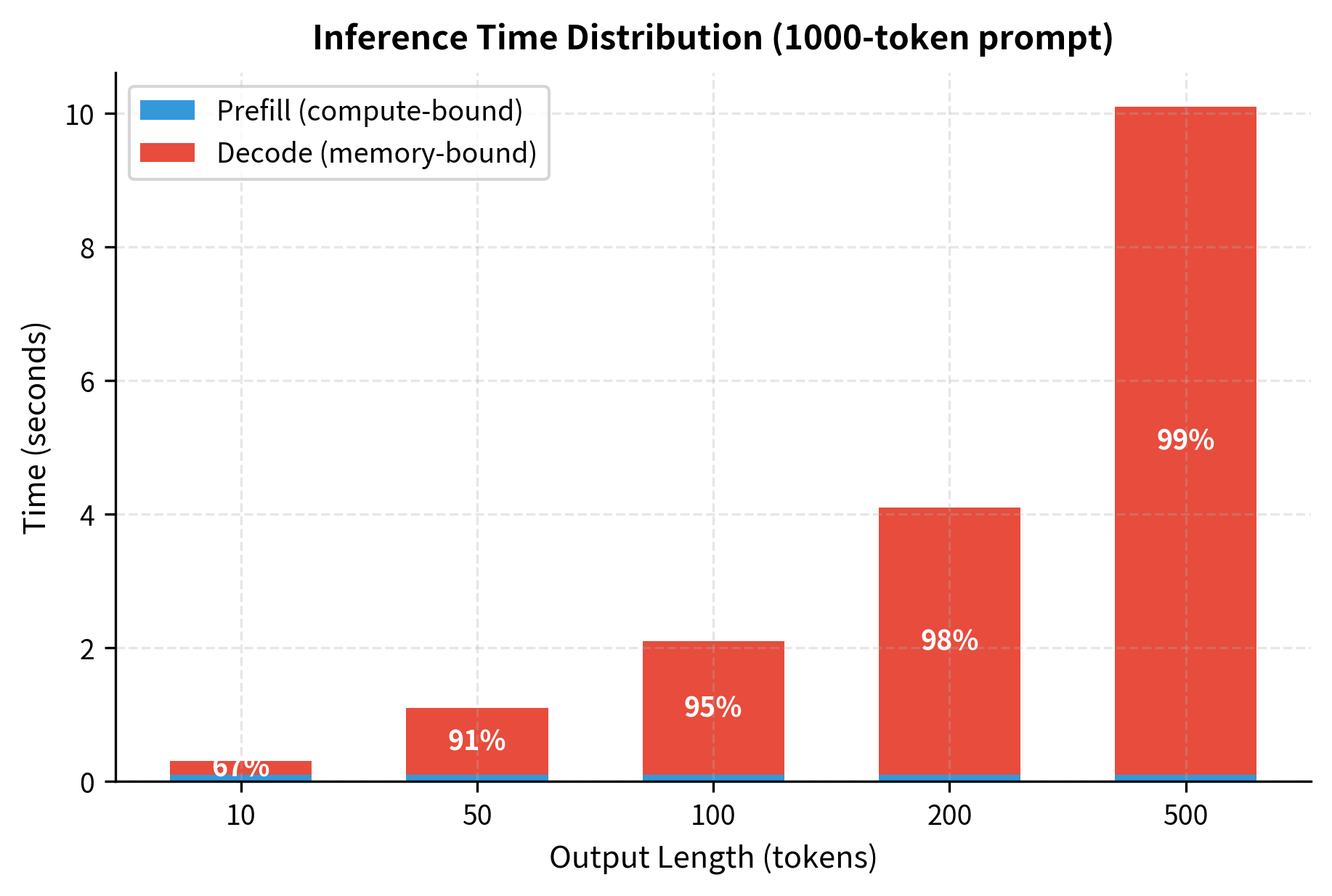
For a typical prompt of 1000 tokens, prefill completes in roughly 100ms. A 10-token response adds 200ms of decode time, making prefill a significant fraction (33%) of total latency. A 500-token response adds 10 seconds of decode time, making prefill negligible (less than 1%). This dramatic shift means optimization priorities should align with your actual request distribution. If most requests generate short outputs, optimizing prefill matters more. If most requests generate long outputs, decode optimization dominates.
Time-to-First-Token Optimization
Many applications stream responses to users, making time-to-first-token (TTFT) the primary latency metric that determines perceived responsiveness. When a user sends a message in a chat interface, TTFT measures the time from submission until the first word of the response appears. Users perceive systems with low TTFT as fast and responsive, even if total generation time is similar.
TTFT measures the time from request arrival until the first generated token is available to the client. This encompasses several distinct stages, each offering optimization opportunities:
- Queue Time: How long the request waits before processing begins. Reducing queue time requires either more capacity (scaling) or smarter scheduling (prioritization).
- Tokenization: Converting the prompt text to token IDs. While typically fast, this step runs on CPU and can bottleneck under high load.
- Prefill Duration: Processing all prompt tokens to populate the KV cache. For long prompts, this dominates TTFT.
- First Decode Step: Generating the first output token. This is typically fast since it's a single forward pass.
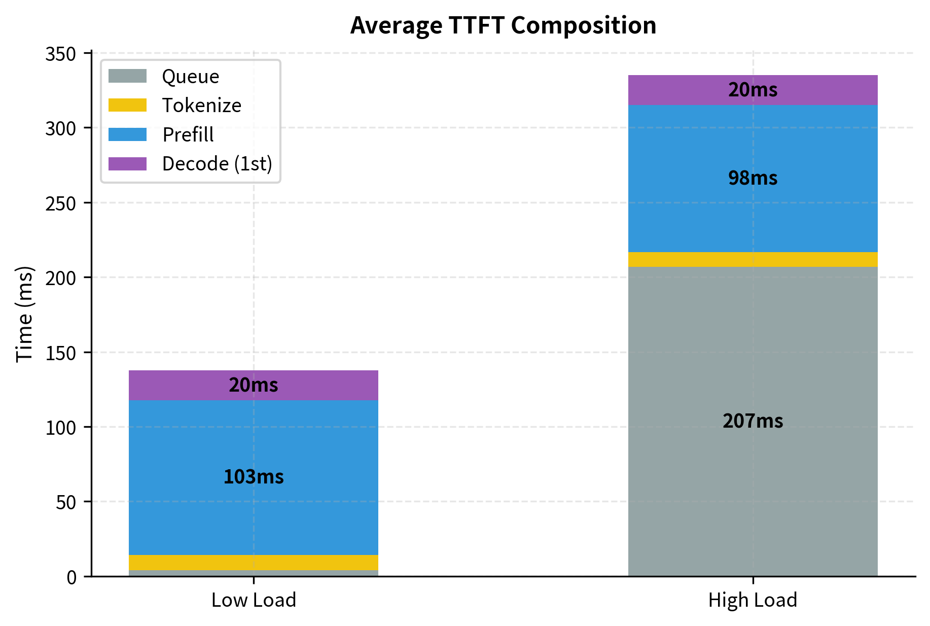
The analysis reveals how bottlenecks shift with load. Under low load, prefill dominates TTFT because queue times are minimal and requests begin processing immediately upon arrival. Optimizing prefill speed through better hardware or chunking would improve TTFT in this regime. Under high load, queue time becomes the dominant bottleneck: requests spend most of their time waiting, not processing. In this regime, improving prefill speed won't help much because requests are already waiting; adding capacity or improving scheduling would be more effective. This analysis guides optimization investments toward the actual bottleneck rather than optimizing components that aren't limiting.
Latency-Throughput Trade-offs
Optimizing for latency often conflicts with optimizing for throughput because the techniques that improve one typically harm the other. Larger batches improve GPU utilization and throughput: processing 32 requests in one batch uses GPU compute more efficiently than processing them one at a time. However, larger batches increase latency for individual requests because each request waits for the batch to form and then shares compute time with other requests in the batch.
The optimal operating point depends on your SLA requirements and cost constraints:
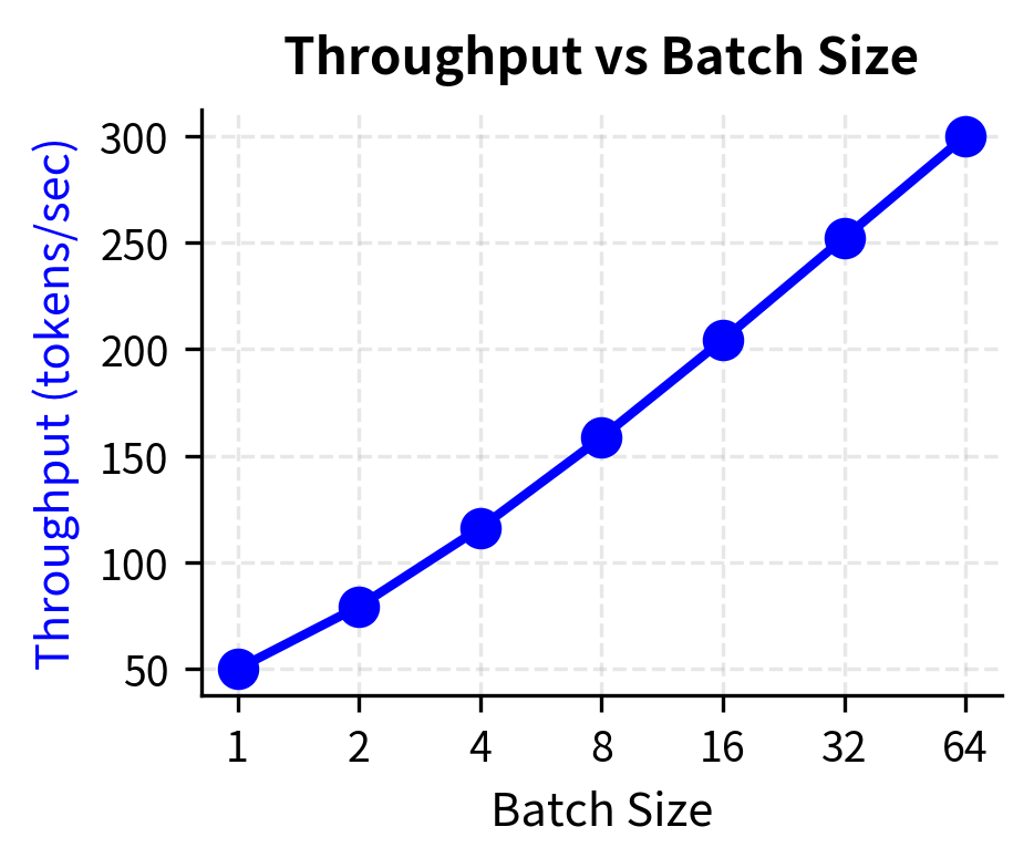
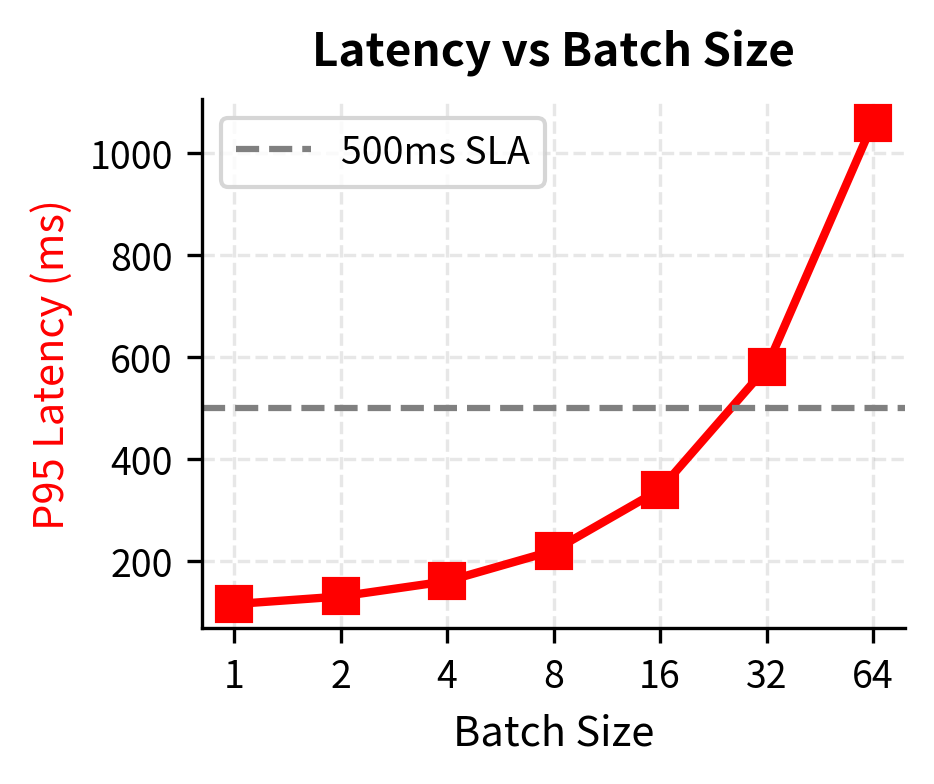
If your SLA requires P95 latency under 500ms, you're constrained to batch sizes below approximately 32 in this scenario. Larger batches would improve throughput (and thus cost efficiency) but violate the latency requirement. The continuous batching techniques from the previous chapter help navigate this trade-off by allowing different requests to enter and exit batches dynamically, improving throughput while limiting how long any individual request must wait.
Monitoring and Observability
Production inference systems require comprehensive monitoring to maintain service quality and debug issues. Without visibility into system behavior, operators cannot distinguish between capacity problems, model issues, and infrastructure failures. Good observability enables proactive intervention before users experience degraded service.
Key Metrics
Effective monitoring tracks metrics at multiple levels, from individual request performance to aggregate system health to business outcomes:
Request-level metrics:
- Time to first token (TTFT): measures perceived responsiveness for streaming applications
- Total latency: measures end-to-end completion time for batch processing use cases
- Tokens per request (prompt and generated): indicates request complexity and resource consumption
- Error rates by error type: distinguishes between timeouts, out-of-memory, and other failure modes
System-level metrics:
- GPU utilization and memory usage: indicates whether hardware is being used efficiently
- Queue depth over time: reveals demand patterns and capacity mismatches
- Active batch size: shows how effectively batching is working
- KV cache utilization: indicates memory pressure and potential for cache eviction
Business-level metrics:
- Requests per second: measures overall demand and system scale
- Tokens per second: measures actual work being done, accounting for request size variation
- Cost per 1000 tokens: combines infrastructure cost with throughput for economic analysis
- SLA compliance rate: the ultimate measure of whether the system meets its commitments
SLOs and Alerting
Service Level Objectives (SLOs) define target performance thresholds that the system should maintain. SLOs translate business requirements (users expect responsive service) into measurable technical targets (P95 latency under 5 seconds). Common SLOs for inference services include:
- Availability: 99.9% of requests succeed (allows approximately 8.7 hours of downtime per year). This SLO accounts for both planned maintenance and unexpected failures.
- Latency: P95 latency below 5 seconds ensures that even unlucky requests complete in reasonable time.
- TTFT: P95 time-to-first-token below 500ms ensures users perceive the system as responsive.
- Error rate: Less than 0.1% of requests return errors, ensuring high reliability for applications built on the inference service.
Alerting should trigger when metrics approach SLO thresholds, not just when they're breached. Alerting only on violations means users have already experienced degraded service by the time operators learn of the problem:
The monitor verifies that all performance metrics currently satisfy their service level objectives. By implementing both warning thresholds (at 80% of the SLO) and critical thresholds (at 100%), the system provides early indications of degrading performance before actual SLA violations occur. Warning alerts give operators time to investigate and potentially scale up or address issues before users experience violations. Critical alerts indicate that the SLA has already been breached and immediate action is required.
Putting It Together: A Complete Serving Pipeline
Let's implement a simplified inference serving pipeline that combines the concepts from this chapter. This example demonstrates how request handling, streaming responses, concurrency limits, and metrics collection work together in a complete system:
This simulation demonstrates the key components working together in a realistic pattern: requests arrive at varying rates following a Poisson process, queue when the server is at capacity (limited to 5 concurrent requests), stream responses as tokens generate, and metrics accumulate for monitoring. The async design allows concurrent request processing while respecting capacity limits, and the streaming response pattern provides tokens to clients as soon as they're available rather than waiting for complete generation.
Key Parameters
The key parameters for the inference server simulation are:
- max_concurrent: Maximum number of requests the server processes simultaneously. Requests beyond this limit are queued, which increases their TTFT but prevents overwhelming the model or running out of GPU memory.
- tokens_per_second: The rate at which the model generates tokens during the decode phase. Higher values indicate faster hardware or more efficient implementation.
- arrival_rate: The average number of requests arriving per second. When arrival rate exceeds processing rate, queues build up and latency increases.
Limitations and Practical Considerations
Inference serving for LLMs remains challenging despite sophisticated techniques. Several fundamental tensions persist that operators must navigate based on their specific requirements:
Cost vs Latency: GPU instances are expensive, but maintaining low latency requires spare capacity. Running at high utilization saves money but increases queue times and latency variance because there's no buffer for traffic spikes. Organizations must balance these competing priorities based on their SLAs and budget constraints. Auto-scaling helps but introduces its own costs (warm pool instances consume resources even when idle) and latency (cold starts delay capacity increases).
Batching Trade-offs: Continuous batching improves throughput significantly by amortizing GPU memory bandwidth across multiple requests, but it complicates request prioritization and debugging. When requests share batches, attributing latency to individual requests becomes harder because each request's timing depends on what else is in the batch. Strict SLA requirements may force smaller batches, sacrificing efficiency for predictability.
Tail Latency: While median latency is often acceptable, P99 latency can be dramatically higher due to garbage collection pauses, occasional long requests that monopolize resources, and resource contention with other workloads. Achieving consistent tail latency requires overprovisioning and careful attention to outlier requests that could delay others.
Model Updates: Deploying new model versions without downtime requires careful orchestration. Blue-green deployments maintain two complete environments and switch traffic between them. Canary releases gradually shift traffic to new versions while monitoring for regressions. Both approaches require infrastructure support and add operational complexity. Rollbacks must be fast when new versions underperform.
Multi-Tenancy: Shared infrastructure serving multiple customers introduces isolation challenges. One customer's burst of long requests shouldn't degrade service for others who are paying for the same SLAs. Token-aware load balancing and request queuing help, but perfect isolation requires separate instances, which increases cost.
The techniques covered in this part (KV caching, quantization, speculative decoding, continuous batching) address many of these challenges, but their interaction with serving infrastructure requires careful tuning. Optimizing a single request's inference speed differs from optimizing system-wide throughput under concurrent load. A technique that improves single-request latency might harm throughput under load, or vice versa.
Summary
This chapter covered the infrastructure layer that transforms trained language models into production services. The key concepts include:
Inference server architecture comprises specialized components including request handlers, schedulers, model executors, and memory managers. Modern servers like vLLM and TGI implement sophisticated features like PagedAttention and continuous batching out of the box.
Request routing determines which model instance handles each request, supporting version-based routing for A/B testing, capability-based routing for cost optimization, and priority routing for SLA differentiation. Health checks ensure routing decisions reflect actual endpoint availability.
Load balancing for LLMs requires token-aware approaches that account for variable request costs. Traditional least-connections balancing fails to capture the difference between short and long generations. Session affinity enables KV cache reuse but conflicts with optimal load distribution.
Auto-scaling adjusts capacity based on metrics like queue depth, latency percentiles, and GPU utilization. Cold start latency for LLM instances (often 30-120 seconds) necessitates warm pools and predictive scaling to maintain responsiveness.
Latency optimization requires understanding the distinct prefill (compute-bound) and decode (memory-bound) phases. Time-to-first-token matters for interactive applications, while total latency matters for batch processing. These often require different optimization strategies.
Monitoring tracks request-level metrics (TTFT, latency), system-level metrics (GPU utilization, queue depth), and business metrics (tokens per second, cost). SLO-based alerting provides early warning before service degradation affects users.
These serving concepts build on the inference optimization techniques from earlier chapters in this part. Together, they enable deploying language models that scale from prototype to production, handling thousands of concurrent users while meeting latency and cost targets.
Quiz
Ready to test your understanding? Take this quick quiz to reinforce what you've learned about Inference Serving.

Comments