Grokking: How Neural Networks Suddenly Learn to Generalize

In the previous chapters, we explored how capabilities emerge suddenly in large language models as they scale. But emergence isn't limited to scale. Sometimes, neural networks exhibit a different kind of sudden transition, a dramatic shift from memorization to generalization. This phenomenon, called grokking, occurs through extended training and challenges our intuitions about when and how neural networks learn to generalize.

The standard wisdom in deep learning suggests that once a model has overfit the training data, continuing to train will only make things worse. Validation accuracy flatlines or degrades while training loss stays near zero. Yet in 2022, researchers at OpenAI discovered something surprising. Small neural networks trained on simple algorithmic tasks would suddenly snap into generalization, sometimes millions of steps after achieving perfect training accuracy. The model would appear hopelessly overfit, memorizing every training example. Then test accuracy suddenly jumped from near chance to near perfect.

In this chapter, we examine grokking in depth. We explore the arithmetic tasks where it was first discovered, competing theories for why it occurs, the phase transitions characterizing grokking dynamics, and what this phenomenon reveals about neural network learning.

Traditional machine learning theory suggests a model's generalization ability is determined early in training. Once the model starts overfitting, the gap between training and test performance should widen. The textbook advice is clear, stop training when validation loss starts increasing, or you will hurt generalization. This guidance emerges from decades of experience with classical statistical models, where the relationship between training time and generalization follows predictable patterns. Grokking violates this expectation completely. Networks exhibiting grokking show something different. Instead of overfitting progressively worsening with continued training, the relationship between memorization and generalization is far more nuanced than traditional theory suggests. Networks can maintain multiple internal solutions, with the dominant solution shifting over time based on regularization and continued optimization. A typical grokking training curve exhibits three distinct phases.

1. Memorization phase, Training accuracy quickly reaches 100%, and training loss approaches zero
2. Plateau phase, Validation accuracy remains at chance level for an extended period (thousands to millions of steps)
3. Grokking phase, Validation accuracy suddenly jumps, quickly approaching training accuracy

The delay between memorization and generalization can be enormous, far exceeding what any standard learning curve would predict. In some experiments, models trained for 10,000 steps show no generalization, but by step 100,000 or 1,000,000, they suddenly achieve near-perfect test accuracy. This dramatic temporal gap shows that generalization and memorization can coexist. The generalizing solution emerges slowly beneath the surface while the memorizing solution dominates the model's observable behavior. The network develops two parallel representations: one stores training examples, another gradually discovers underlying task structure. Eventually, structural understanding becomes dominant.

The original grokking paper focused on small algorithmic datasets, particularly modular arithmetic. These tasks provide an ideal testbed because:

• They have clean mathematical structure
• The dataset size is precisely controllable
• Perfect generalization is achievable (the function is learnable)
• The solutions have interpretable structure

The choice of modular arithmetic is particularly elegant: it represents one of the simplest possible algorithmic tasks where the rules are completely deterministic, the input space is finite and well-defined, and there exists a compact closed-form solution that any sufficiently expressive model should theoretically be able to learn. This makes modular arithmetic the ideal laboratory for studying the fundamental dynamics of how neural networks transition from memorization to algorithmic understanding.

The canonical grokking task is modular addition: given two numbers $a$ and $b$, compute $(a + b) \mod p$ for some prime $p$. This operation lies at the heart of many cryptographic systems and represents one of the most basic operations in abstract algebra: it is both practically relevant and mathematically well-understood.

The modulo operation computes the remainder when the sum of two numbers is divided by $p$. The modulo operation captures the idea of "clock arithmetic", values wrap around after reaching a maximum. For example, $(50 + 60) \mod 97 = 13$ because $50 + 60 = 110 = 1 \times 97 + 13$, so the remainder when dividing by 97 is 13. The key insight is that results are always constrained to lie within the range from 0 to $p-1$, creating a finite cyclic structure.

Parameters:

• $a$, the first operand (an integer from 0 to $p-1$)
• $b$, the second operand (an integer from 0 to $p-1$)
• $(a + b)$, the sum of the two operands (computed before applying the modulo operation)
• $\mod p$, the modulo operation that returns the remainder after division by $p$, ensuring the result stays within the range $[0, p-1]$
• $p$, a prime number defining the modular arithmetic system, which creates the wraparound behavior

With $p = 97$, there are $p \times p = 97 \times 97 = 9409$ possible input pairs, each mapping to one of 97 outputs. This creates a dataset of manageable size that is small enough for rapid experimentation yet large enough that pure memorization requires substantial model capacity.

Prime numbers ensure that modular arithmetic forms a field, where every non-zero element has a multiplicative inverse. This gives the task clean, learnable patterns without special cases. When the modulus is composite (not prime), certain numbers share common factors with the modulus, creating irregular patterns that complicate division and multiplication. Prime moduli provide the cleanest structure for the network to discover.

The task is framed as sequence modeling to leverage the transformer architecture. The input sequence is [a, b, =], and the target is the result. The transformer learns to predict the correct output given the input tokens representing the operands. This framing lets you study grokking using the same architectures that power modern language models, making the insights applicable to understanding broader neural network behavior.

With 9,409 total possible input pairs, the 50/50 train-test split provides 4,704 training examples and 4,705 test examples. This balanced partition ensures the model must genuinely generalize to unseen combinations rather than simply memorizing the training set. The sample outputs demonstrate the modular wraparound behavior where sums exceeding the modulus (97) cycle back to smaller values, a fundamental property the model must learn to capture. The sample outputs demonstrate this wraparound behavior, which the network must learn to internalize for true generalization.

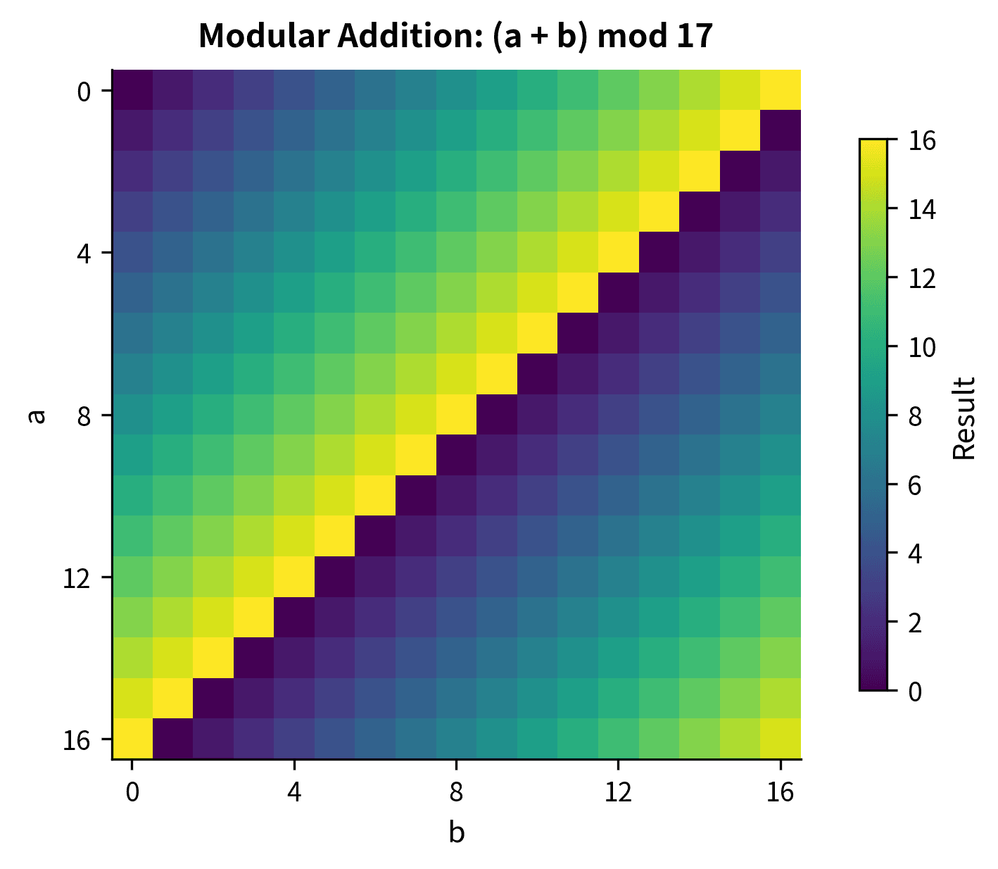
The heatmap reveals the striking diagonal pattern in modular addition. Each diagonal stripe represents outputs with the same value, and these stripes wrap around at the boundaries due to the modular operation. This visual structure shows what the network must learn: the output depends only on the sum of the inputs modulo the prime, not on memorizing individual input-output pairs.

With only 50% of the data for training, the network must generalize to unseen input combinations. A model that merely memorizes the training pairs will achieve 50% accuracy on the test set at best (since half the pairs are held out). This setup creates a clean distinction between memorization and generalization: a model that has truly learned the addition algorithm will succeed on any valid input pair, while a model that has merely memorized will fail on the held-out examples.

Following the original grokking experiments, we use a small transformer to learn these arithmetic patterns. The transformer architecture is particularly well-suited for this task. Its attention mechanism can learn to route information between the two input operands, and its feedforward networks can learn the computational operations needed to combine them.

The key to observing grokking is weight decay (L2 regularization). Without it, the model memorizes the training data and never generalizes. With appropriate weight decay, grokking emerges. This reveals a fundamental aspect of grokking: the phenomenon requires balance between the model's capacity to memorize and the regularization pressure favoring simpler, generalizable solutions. Weight decay pulls parameters toward zero, penalizing the complex configurations that memorization requires while leaving simpler algorithmic solutions relatively unaffected.

The training completes 300 epochs, which provides sufficient iterations to observe the initial phases of grokking behavior. While full grokking convergence may require 10,000 or more epochs depending on random initialization, this training duration captures the early memorization phase and the beginning of the transition toward generalization.

The final metrics show the model's state after 300 epochs of training. The training accuracy approaching 1.0 confirms successful memorization of the training set, while the test accuracy value indicates the degree of generalization achieved at this point in training.

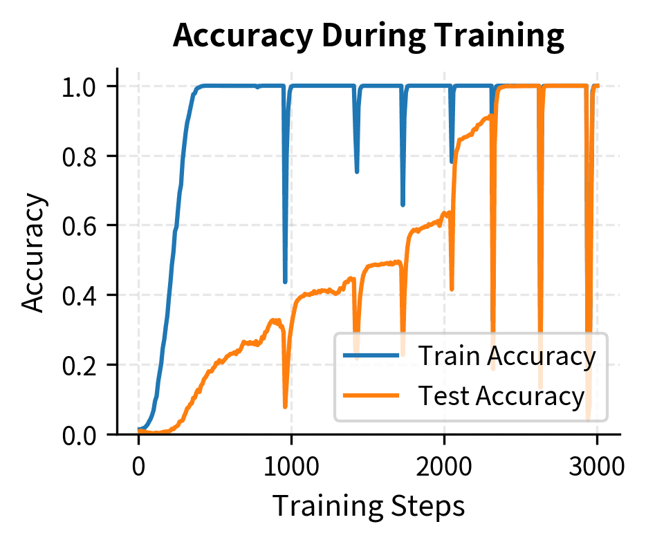
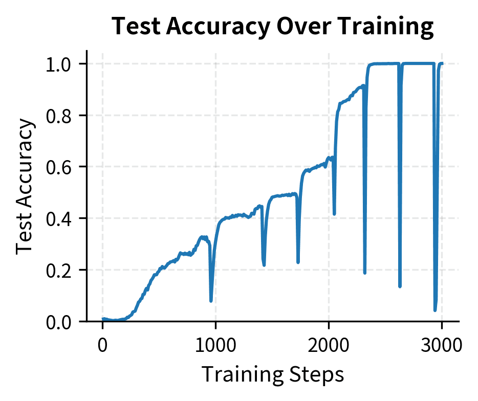
The training curve reveals the signature grokking pattern. Training accuracy reaches near 100% within the first few hundred epochs as the model memorizes the training examples, with training loss dropping to near zero. Meanwhile, test accuracy starts low and begins climbing as the model transitions from pure memorization toward generalization. In longer training runs, test accuracy would eventually match training accuracy, demonstrating complete grokking.

This delay can be dramatic. In the original grokking paper, some experiments required training for over $10^5$ steps after the model had memorized the training data before generalization emerged.

Why does grokking happen? Several theories have been proposed, each offering partial insight into this phenomenon. These theories illuminate different aspects of the same underlying process, revealing the complexity of neural network learning and how multiple forces shape representation evolution during training.

One influential explanation comes from mechanistic interpretability research. According to this view, neural networks can represent solutions in multiple ways. One is a memorization circuit that stores input-output pairs explicitly, another is an algorithm circuit that computes the correct answer using the underlying mathematical structure. These two circuits can coexist within the same network. Their relative strengths determine the model's behavior at any given point in training.

For modular addition, the algorithmic solution represents numbers as points on a circle. Since modular arithmetic wraps around, the network can compute their sum using trigonometric relationships. Addition modulo $p$ has inherent circular structure: it resembles how a clock cycles from 12 back to 1. By embedding numbers as points on a circle, the network can exploit this geometric structure directly. The model can learn embeddings where each number $k$ maps to a point on the unit circle.

To understand this formula intuitively, imagine a clock face divided into $p$ equal sections rather than 12. This embedding places each number at a unique position on the unit circle, evenly spaced around the circumference. The number 0 sits at the rightmost point (the 3 o'clock position), and as $k$ increases, you move counterclockwise around the circle. The angle for number $k$ is $\frac{2\pi k}{p}$ radians, which divides the full circle (2π radians) into $p$ equal segments. Dividing by $p$ gives us the angular spacing between consecutive numbers. This representation captures the wraparound property because when numbers are embedded on a circle, adding two numbers becomes geometrically equivalent to adding their angles.

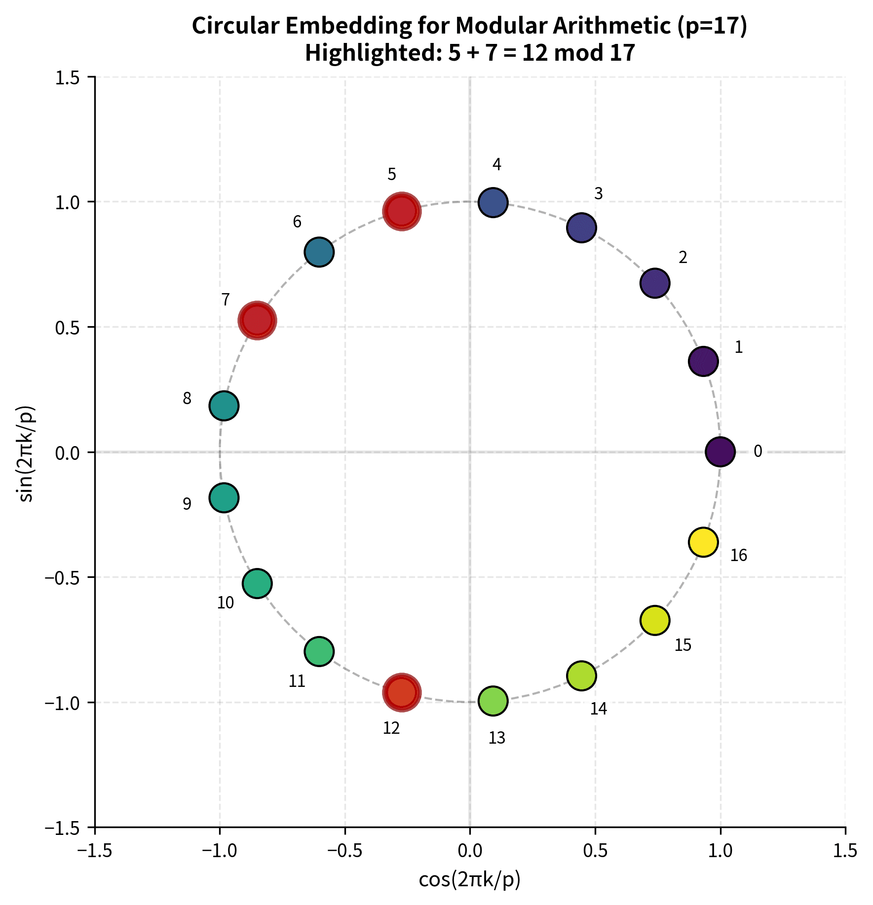
The visualization shows how numbers 0 through 16 are evenly distributed around the unit circle. The highlighted points (5, 7, and 12) demonstrate how addition works geometrically: adding 5 and 7 corresponds to combining their angular positions, resulting in the position for 12. This circular structure is what the network must discover during grokking to achieve true generalization.

Parameters:

• $p$, the prime modulus defining the arithmetic system
• $k$, the number being embedded (an integer from 0 to $p-1$)
• $\text{embedding}(k)$: a two-dimensional vector representing $k$ as a point on the unit circle
• $\cos\left(\frac{2\pi k}{p}\right)$: the x-coordinate of the point (horizontal position on the circle ranging from -1 to 1)
• $\sin\left(\frac{2\pi k}{p}\right)$: the y-coordinate of the point (vertical position on the circle ranging from -1 to 1)
• $\frac{2\pi k}{p}$: the angle in radians that maps number $k$ to its position on the circle

This circular representation captures the wraparound property of modular arithmetic. After reaching $p-1$, the next value, 0, is adjacent on the circle, making addition correspond to rotation.

This representation naturally captures the wraparound property of modular arithmetic. After $p-1$, the next value 0 appears adjacent on the circle, making the structure cyclic rather than linear. The circular embedding ensures numbers close in modular arithmetic are also close in the embedding space, enabling the network to learn smooth, generalizable functions instead of storing separate parameters for each input.

Consider what happens when we add $a$ and $b$ in this circular representation. Each number corresponds to a specific angle around the circle, and their sum corresponds to the angle you reach by first rotating to angle $a$ and then rotating by an additional angle $b$. The operation $(a + b) \mod p$ corresponds to rotating from angle $\frac{2\pi a}{p}$ by an additional $\frac{2\pi b}{p}$ radians. The modular wraparound happens automatically because angles naturally wrap around: rotating by more than $2\pi$ radians brings you back around the circle. Mathematically, this is expressed as:

Key components of this calculation:

Parameters:

• $\text{angle}(a + b)$, the resulting angle after adding $a$ and $b$ on the circle (representing the sum in the circular embedding space)
• $\frac{2\pi a}{p}$, the angle corresponding to number $a$ (its position on the circle)
• $\frac{2\pi b}{p}$, the angle corresponding to number $b$ (its position on the circle)
• $\frac{2\pi(a + b)}{p}$, the combined angle (which naturally wraps around at $2\pi$ and captures the modular arithmetic behavior where values cycle back to 0 after reaching $p$)

This geometric operation can be computed using attention mechanisms that learn to compose these rotations through the transformer's query-key-value operations, creating a compact algorithmic solution rather than requiring separate parameters for each possible input pair. The key advantage of this approach is that it requires only a constant number of parameters regardless of the number of possible input pairs, since the same rotation operation applies to all inputs.

During training,

1. The memorization circuit forms first because it's the fastest path. Gradient descent quickly finds a way to map each seen training example to its correct output.
2. The algorithm circuit develops slowly in parallel: The correct representations and computations require coordinated changes across multiple layers.
3. Weight decay gradually penalizes the memorization circuit more heavily than the algorithm circuit: Memorization requires storing many parameters (one pattern per example) while the algorithm is more compact.
4. Eventually, the algorithm circuit becomes strong enough to dominate: generalization emerges.

This view explains why weight decay is essential for grokking: it provides the pressure that eventually favors compact, generalizing solutions over sprawling memorization.

A related perspective focuses on how representation learning drives grokking. The model must discover that numbers in modular arithmetic have circular structure. This involves learning embeddings with these properties:

• Numbers close in modular distance are close in embedding space.
• The embedding captures the cyclic nature of modular arithmetic (where 0 is close to $p-1$).
• Addition corresponds to a composable operation in this space (via rotation).

Learning such structured representations takes time:

• Random initialization places numbers without meaningful structure.
• Memorization requires only the ability to distinguish training examples, not good representations.
• Gradient signals for better representations are weak initially because memorization already achieves low training loss.

Only after extended training do the cumulative effects of weight decay and gradient updates align the representations with the mathematical structure.

Information-theoretic views frame grokking as compression. A memorizing solution has high description length, as it must store each training example separately. An algorithmic solution has low description length, as it only needs to store the rules for addition.

Weight decay acts as a description length penalty, favoring solutions that use fewer bits. The network starts by memorizing because it's the fastest way to reduce training loss. But as training continues, the regularization pressure drives the network toward more compressed representations. Grokking occurs when the compressed solution finally achieves competitive training loss.

This connects to the principle of Occam's razor and minimum description length (MDL) in learning theory: given two hypotheses that explain the data equally well, prefer the simpler one. Weight decay operationalizes this preference.

Another framework distinguishes between lazy and rich learning regimes. In the lazy regime, the network makes minimal changes to its initial representations, essentially performing kernel regression, while in the rich regime, representations change substantially, adapting to the structure of the task.

Grokking may represent a phase transition from lazy to rich learning. The transition unfolds as follows:

1. Early training operates in the lazy regime, where the network memorizes using representations close to initialization
2. Continued training with regularization eventually pushes the network into the rich regime
3. In the rich regime, representations restructure to capture the underlying algorithm

This transition takes time because escaping the lazy regime requires overcoming an energy barrier. The network must temporarily perform worse on training data as it reorganizes its representations before achieving better generalization.

Grokking exhibits sharp phase transition behavior characteristic of many complex systems. The transition from non-generalization to generalization is not gradual: it happens suddenly over a relatively small number of training steps compared to the total training time. This sharp transition distinguishes grokking from standard learning curves, where test accuracy typically improves smoothly alongside training accuracy. The suddenness suggests that grokking represents a qualitative change in the network's internal organization rather than a quantitative accumulation of knowledge.

Several factors influence when grokking occurs:

Factors:

• Weight decay strength: Controls regularization pressure. Too little means the model memorizes without grokking; too much causes underfitting. A critical range exists where grokking reliably occurs.
• Training data fraction: Affects the memorization-generalization tradeoff. More training data accelerates grokking by strengthening the signal for generalization, while less training data delays or prevents grokking because memorization becomes cheaper relative to generalization.
• Model capacity: Plays a complex role. Very small models may lack capacity for memorization or the algorithm, while very large models memorize so easily that regularization cannot overcome it. The optimal range allows representing both solutions, giving regularization time to favor generalization.

The experiments train four separate models with weight decay values ranging from 0.01 to 2.0, each for 150 epochs. This comparison reveals how regularization strength affects the timing and occurrence of the grokking transition. The final accuracy values show how different regularization strengths lead to varying degrees of generalization, with intermediate values typically achieving the best balance between memorization and generalization.

The relationship between weight decay and grokking speed illustrates the phase transition nature of the phenomenon. At low weight decay, the model memorizes and stays memorized. As weight decay increases, grokking appears and happens progressively faster. Beyond some threshold, strong regularization can interfere with learning entirely.

The optimizer influences grokking dynamics. The decoupled weight decay in AdamW provides cleaner regularization than L2 regularization implemented as a loss term. This distinction matters for grokking: AdamW tends to produce more reliable grokking behavior because the weight decay acts uniformly rather than being scaled by the adaptive learning rates.

Learning rate also matters: higher learning rates can accelerate the phase transition once it begins but may also cause instability, while lower learning rates lead to slower but more stable grokking. There's evidence that learning rate schedules, particularly warmup followed by decay, can improve grokking reliability.

We can quantify the sharpness of the grokking transition by looking at the rate of change of test accuracy. Rather than examining raw accuracy values, which tell us where the model is, examining the derivative reveals how quickly the model is improving at each point in training. This derivative perspective helps distinguish between gradual improvement and the sudden transitions characteristic of grokking.

where:

• $\text{accuracy}$, the test accuracy at a given point in training (a value between 0 and 1)
• $\text{step}$, the training step number (counting gradient updates or epochs)
• $\frac{d(\text{accuracy})}{d(\text{step})}$, the derivative showing how quickly accuracy changes per training step (representing the instantaneous rate of improvement measured in accuracy units per step)

This derivative measures the instantaneous rate at which test accuracy improves during training. To interpret this quantity, think of it as the slope of the accuracy curve at any given moment. A large positive value indicates rapid improvement, meaning the model is quickly getting better at the task. Values near zero indicate periods of stagnation where accuracy remains roughly constant despite continued training. During grokking, the derivative shows a distinctive pattern: it stays near zero during the plateau phase, spikes dramatically during the transition, then returns to near zero after full generalization. These peaks characterize the transition from memorization to generalization. This concentration of improvement within a narrow window of training steps is what makes grokking visually striking on learning curves, distinguishing it from gradual learning where the derivative would remain relatively constant. The sharper the spike, the more abrupt the transition from memorization to generalization.

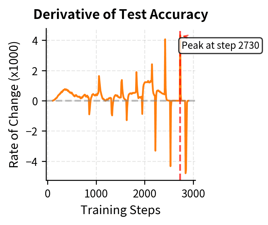
The derivative plot provides a quantitative view of the learning dynamics. Peaks in the rate of change show when the model's test accuracy is improving most rapidly. The location and magnitude of these peaks help characterize the transition from memorization to generalization. The sharp spike in $\frac{d(\text{accuracy})}{d(\text{step})}$ during the transition indicates that grokking involves rapid improvement concentrated within a small window of training steps. This contrasts with gradual steady progress, where improvement would be distributed more evenly across training. The mathematical signature of grokking is therefore not just high eventual accuracy, but this distinctive pattern of delayed-then-rapid improvement. We can quantify this transition by computing key metrics: memorization step (when training accuracy exceeds 99%), grokking step (when test accuracy exceeds 90%), and maximum acceleration (the sharpest improvement point). This numeric characterization enables comparison across different hyperparameter settings.

These metrics quantify the grokking transition in concrete numerical terms. The delay between memorization (when training accuracy exceeds 99%) and grokking (when test accuracy exceeds 90%) reveals how long the model remains in the plateau phase before generalization emerges. This delay, often spanning thousands or millions of steps, is the defining characteristic of grokking and distinguishes it from standard learning curves where generalization tracks training performance closely. By measuring this delay explicitly, we can compare grokking behavior across different hyperparameter settings and gain quantitative insight into the factors that accelerate or delay the transition.

The delay between memorization and grokking can be substantial. In our demonstration, grokking occurs relatively quickly due to the small scale, but in larger experiments, this delay can span orders of magnitude in training time.

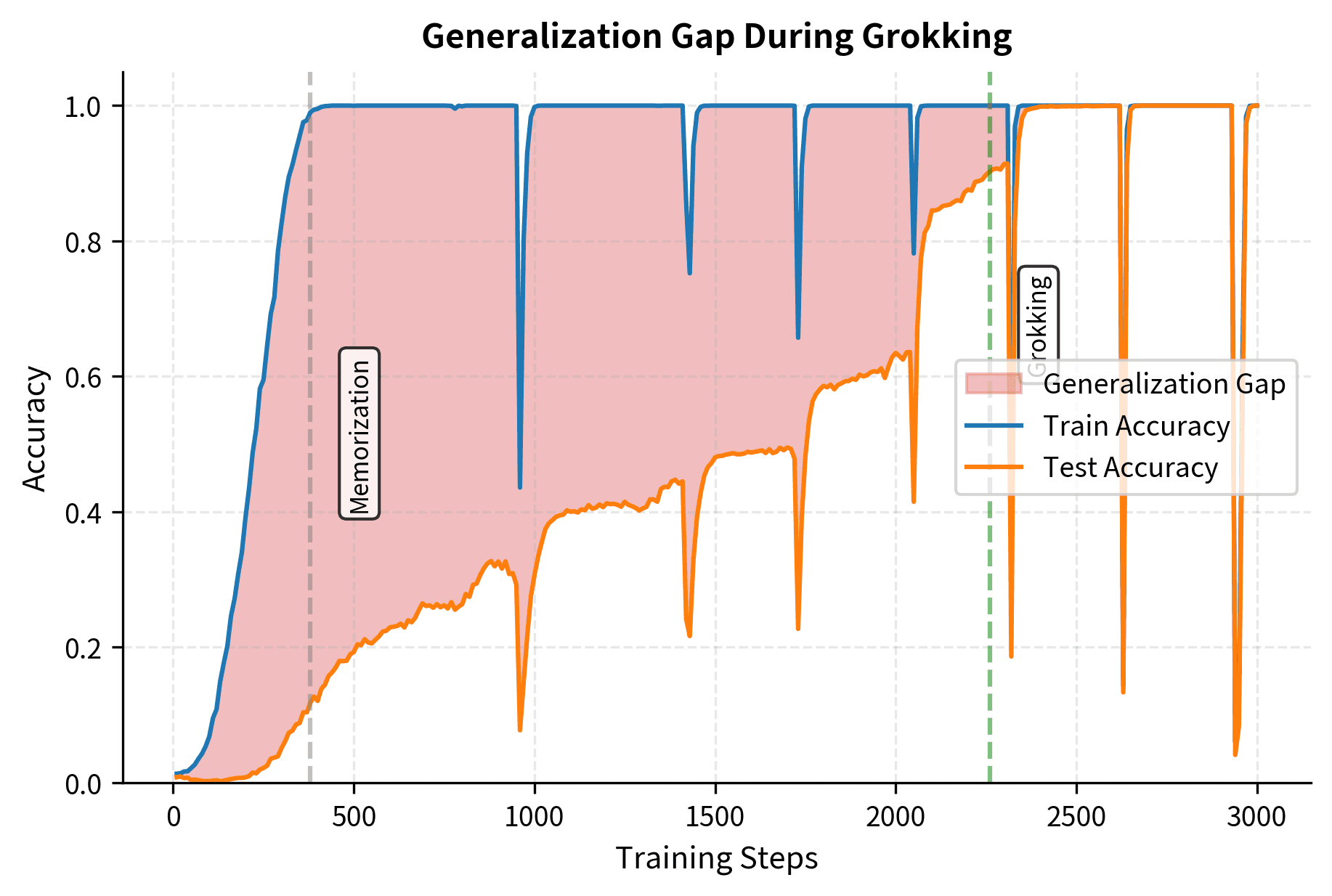
This visualization shows the generalization gap, the difference between training and test accuracy, throughout training. The shaded region represents how much better the model performs on training data than test data. During memorization, this gap grows rapidly as the model achieves high training accuracy while test accuracy remains low. The gap remains large during the plateau phase. Finally, during grokking, the gap shrinks dramatically as test accuracy catches up to training accuracy.

Parameters:

• vocab_size, Size of the token vocabulary (p + 1 for numbers 0 to p-1 plus the equals token)
• d_model, Dimension of embeddings and hidden states (128 in our experiments)
• nhead, Number of attention heads (4 heads allow the model to attend to multiple patterns simultaneously)
• num_layers, Number of transformer encoder layers (2 layers provide enough depth for learning the algorithm)
• dim_feedforward, Dimension of the feedforward network in each layer (512, providing capacity for internal transformations)
• dropout, Set to 0.0 because dropout can interfere with observing clean grokking dynamics
• weight_decay, Regularization strength that drives the transition from memorization to generalization (1.0 in our main experiments)
• learning_rate, Step size for optimization (1e-3) balancing training speed with stability
• n_epochs, Number of complete passes through the training data (thousands to millions may be needed to observe grokking)
• train_fraction, Proportion of data used for training (0.5 creates a challenging generalization task by holding out half the input pairs)
• batch_size, Number of examples per training batch (512) providing stable gradients while maintaining computational efficiency

Beyond modular arithmetic, grokking appears in various other settings, including many algorithmic learning tasks:

• Polynomial evaluation: Computing $f(x) \mod p$ for polynomial $f$.
• Sequence completion: Learning rules for continuing sequences.
• Boolean functions: Learning XOR, parity, and other boolean operations.

The common thread is tasks with underlying mathematical structure that can be represented compactly but where memorization provides a competing solution.

Ongoing research examines whether grokking-like phenomena occur in language model training. Several observations suggest this might be happening:

Observations:

• Certain linguistic patterns (such as subject-verb agreement and long-range dependencies) show sudden improvement during training.
• Models sometimes exhibit delayed emergence of grammatical understanding.
• Continued training past apparent convergence sometimes improves specific capabilities.

However, the relationship between these observations and classical grokking remains unclear. Language data lacks the clean mathematical structure of modular arithmetic, making it harder to distinguish grokking from other phenomena, such as capability emergence or curriculum effects in the data.

Grokking connects to the double descent phenomenon discussed earlier. Both involve counterintuitive relationships between training time, model capacity, and generalization:

• Double descent reveals that larger models can generalize better, contrary to classical bias-variance tradeoff predictions
• Grokking reveals that longer training can improve generalization, contrary to early stopping advice

Both suggest that modern neural network training operates in regimes where classical intuitions break down. The interpolation threshold where models can perfectly fit training data, marks a transition to a new generalization regime where more capacity and more training can help rather than hurt.

Understanding grokking has practical implications for training. Don't stop training too early, this prevents generalization. Traditional early stopping monitors validation loss and halts when it increases. If the model is in the pre-grokking regime, validation loss increases might be temporary, and continued training with appropriate regularization can lead to much better generalization.

When designing your training pipeline, consider these more nuanced approaches:

Best practices:

• Train longer with strong regularization.
• Monitor whether validation metrics are still changing, not just their direction.
• Use multiple checkpoints to evaluate later models rather than relying solely on early stopping heuristics.

Grokking requires regularization. Weight decay is the primary enabler, though dropout and data augmentation also help. Regularization provides the pressure to shift from memorization to generalization. Calibrate regularization carefully. Too little means memorization without generalization, while too much causes underfitting. The optimal range allows both solutions to coexist, with regularization favoring generalization.

Grokking behavior depends on the dataset. With more training data, grokking happens faster because there's more signal for the generalizing solution. With less data, grokking takes longer or may not happen at all. This has implications for your data collection and curation. If you're working on a task with underlying structure to learn, provide sufficient diverse examples to help the generalizing solution emerge. Repetitive or redundant data may enable memorization without pushing toward generalization.

The architecture affects grokking dynamics. Attention mechanisms seem particularly amenable to grokking on algorithmic tasks because they can represent the compositional computations these tasks require. Feedforward networks can also grok but may require different hyperparameters.

When working with tasks that have known structure, choose architectures that can represent that structure compactly to accelerate grokking.

This principle connects to broader concepts about inductive biases and architecture design we'll explore throughout this book.

Several aspects of grokking remain poorly understood. The fundamental question is whether we can predict whether and when grokking will occur given a model, dataset, and training configuration. We can make qualitative predictions (such as "more regularization speeds grokking" or "more data helps") but not quantitative ones. We cannot reliably predict whether grokking will happen at step 50,000 or 500,000, or at all.

The relationship between grokking in toy tasks and training dynamics in practical applications remains unclear. Large language models train on natural language with far messier structure than modular arithmetic. Whether grokking insights transfer to these settings is an open question for the broader research community. Some researchers argue that continued training with regularization unlocks better generalization in LLMs. Others suggest the phenomena are fundamentally different at scale.

There are also computational implications. If valuable capabilities emerge only after extended training, we should use longer training runs in practice. However, training is expensive, making it hard to justify continued training when visible metrics have plateaued. Better understanding of when grokking will occur could help justify these extended training investments, but such understanding remains elusive.

Finally, the mechanisms behind grokking are still debated. Circuit formation, representation learning, compression, and phase transitions are all plausible explanations that are not mutually exclusive. Developing a unified theory that predicts grokking from first principles remains an open challenge. Progress in mechanistic interpretability may eventually provide clearer answers by enabling direct observation of internal representations emerging during grokking. We'll encounter this approach in later chapters on model analysis.

This chapter explored grokking, a phenomenon where neural networks suddenly generalize long after memorizing training data.

Key characteristics of grokking:

• Dramatic delay between achieving perfect training accuracy and generalization
• Sharp phase transition from memorization to generalization
• Critical dependence on regularization strength, particularly weight decay
• Clearest observation in algorithmic tasks with mathematical structure

Theoretical explanations:

• Circuit formation: Memorization and algorithmic circuits compete, with regularization favoring the compact algorithm
• Representation learning: Discovering task structure takes time even after memorization
• Compression: Weight decay drives the network toward minimum description length solutions
• Lazy-to-rich transition: Escaping lazy learning requires overcoming an energy barrier toward rich representations

Practical implications:

• Longer training with regularization can unlock generalization that early stopping would prevent
• Regularization strength critically affects whether and when grokking occurs
• More training data accelerates grokking by strengthening signals for generalizing solutions
• Architecture choices affect grokking dynamics through their inductive biases

Grokking challenges the conventional wisdom that treats overfitting and generalization as mutually exclusive. Neural network training can pass through extended phases where memorization dominates before generalization emerges, revealing that our understanding of how neural networks learn is incomplete. Better training practices, regularization strategies, and longer training schedules unlock capabilities hidden by premature stopping.

Ready to test your understanding? Take this quick quiz to reinforce what you've learned about grokking and delayed generalization in neural networks.