Instruction Tuning Training: Data Mixing & Loss Masking

With instruction data prepared and properly formatted, we turn to the training process itself. Instruction tuning makes pre-trained models follow requests and provide helpful responses. This process requires more than standard fine-tuning. You must decide how to mix instruction types, which signals to learn from, and how to keep pre-trained capabilities.

This chapter covers the mechanics of instruction tuning and the decisions required during training. We will look at balancing task types with data mixing, using loss masking to focus the model on responses, selecting hyperparameters, and using multi-task learning to improve generalization.

Instruction tuning datasets contain examples from many task types, such as question answering, summarization, and coding. Each category requires different skills, such as factual recall or logical reasoning. Task distribution determines what the model learns and how it generalizes. You must control this distribution.

Training on all available instruction data causes task imbalance. Instruction datasets are rarely balanced because some tasks are easier to collect than others. Question-answering pairs can be scraped from forums and documentation, while high-quality mathematical reasoning examples require expert annotation. If your dataset contains 120,000 question-answering examples but only 8,000 math examples, the model sees QA tasks 15 times more frequently during training. This imbalance causes the model to perform well on common tasks but struggle with rare ones, even if both are equally important for the application.

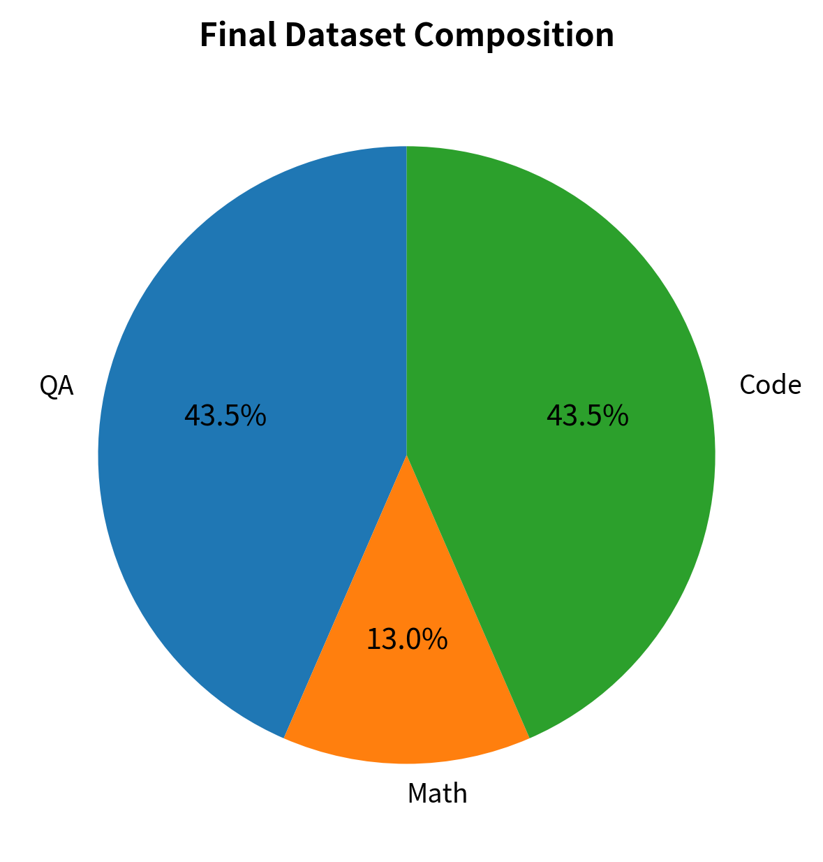
Consider a hypothetical instruction dataset with the following distribution, which reflects the kind of imbalance commonly found in real instruction tuning corpora:

In proportional sampling, where examples are drawn based on their natural frequency, the model sees the QA category roughly 15 times more often than math. This imbalance biases the training signal. For example, after 1 million examples, the model has updated its weights 345,000 times for QA but only 23,000 times for math. The model's parameters are therefore shaped far more by what helps it answer questions than by what helps it solve mathematical problems, even if both are equally important.

Three main approaches address task imbalance, each with different trade-offs that make them suitable for different situations and goals:

Proportional sampling uses the natural data distribution without modification. Examples appear according to their frequency in the dataset, meaning that if 34% of your data is question-answering, then 34% of your training batches will contain question-answering examples on average. This works well if the natural distribution matches your goals, like when a general assistant should handle common tasks more fluently because you perform them more often. The main drawback is underfitting on minority tasks. The model may not see enough math examples to learn reasoning, even if that skill is important.

Equal sampling takes the opposite approach, assigning each task equal probability regardless of dataset size. If you have seven task categories, each receives roughly 14.3% of the training examples. This strategy ensures the model sees rare tasks frequently enough to learn from every category. However, it introduces its own problems: it may waste model capacity by over-training on already well-represented tasks, and more seriously, it can cause severe overfitting when small task datasets must be repeated many times to achieve equal representation. If your math dataset has only 8,000 examples but needs to match 120,000 QA examples, each math example would be seen 15 times, risking memorization rather than generalization.

Temperature-based sampling uses a temperature parameter to balance the task distribution. This approach gives you continuous control between the extremes of proportional and equal sampling. Given raw task proportions $p_i$, the sampling probability becomes:

where:

• $q_i$: the adjusted sampling probability for task $i$, representing how likely you are to draw an example from this task during training
• $p_i$: the raw proportion of task $i$ in the original dataset, calculated as the number of examples in task $i$ divided by the total number of examples
• $p_i^{1/T}$: the exponentiated proportion for task $i$, where the $1/T$ power reduces the differences between large and small values to make the distribution more uniform
• $T$: the temperature parameter that controls distribution smoothing, typically set to values of $T \ge 1$
• $\sum_{j} p_j^{1/T}$: the sum of exponentiated proportions across all tasks, which ensures the adjusted probabilities sum to one

The temperature parameter changes the distribution by exponentiating probabilities. Understanding how it works helps you choose the right setting:

1. When $T = 1$: The exponent is $1$, so $p_i^{1/1} = p_i$, which means $q_i = p_i$. This preserves the original proportional sampling exactly, with no adjustment to the natural distribution.
2. When $T \to \infty$: The exponent approaches $0$. Since any positive number raised to the power of $0$ equals $1$, all weights approach equality. The result is perfectly uniform sampling across all tasks, regardless of their original sizes.
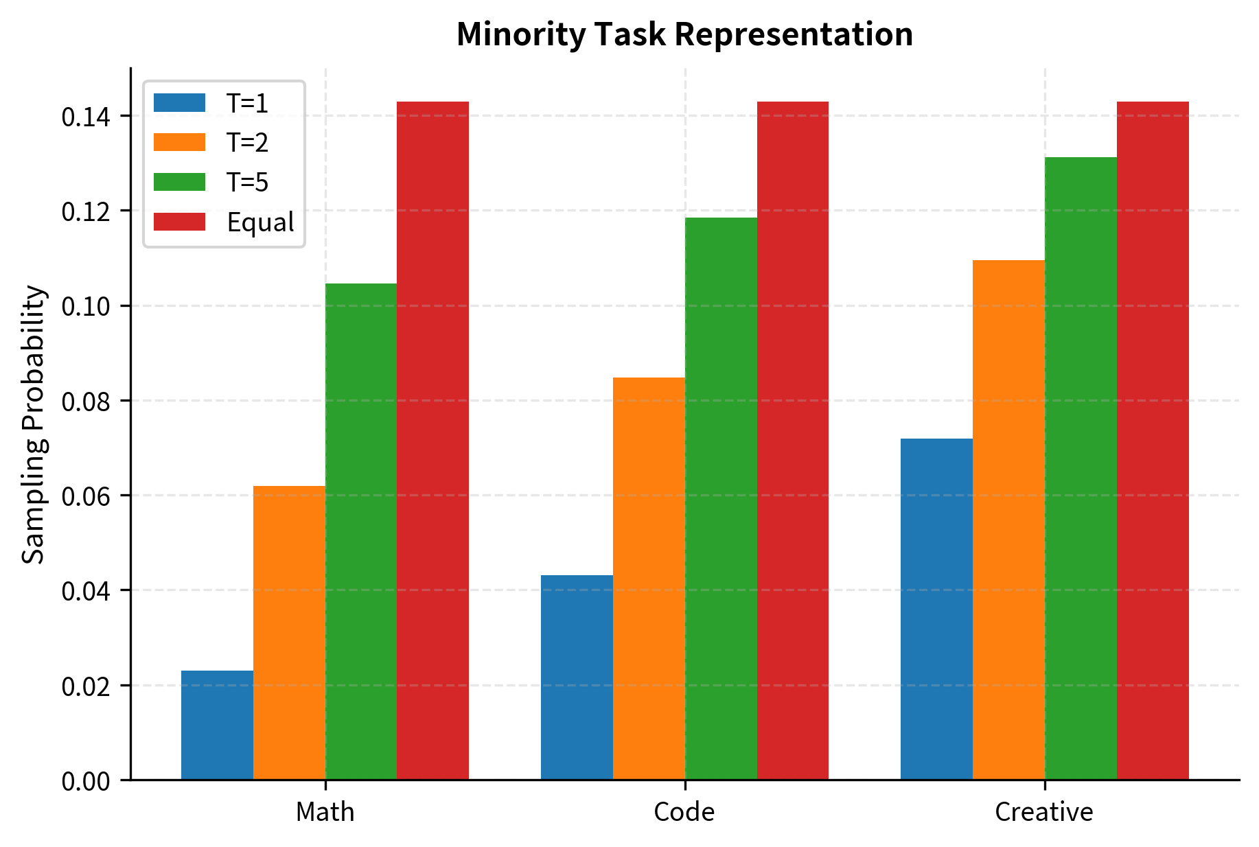
3. When $T \approx 2-3$: The distribution is flattened but not made uniform. Rare tasks are upweighted to ensure they appear frequently enough during training for the model to learn from them, while common tasks are still sampled more frequently than rare ones, reflecting their greater natural occurrence. This intermediate regime often provides the best balance in practice.

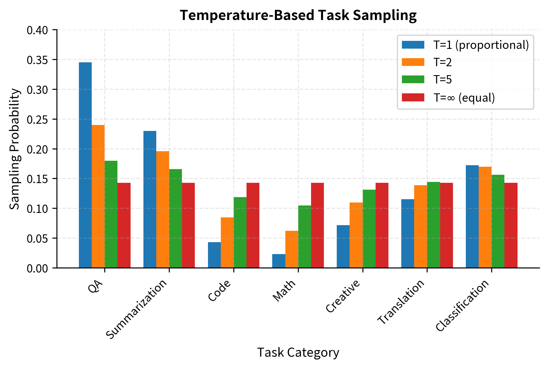
Research from instruction tuning papers like FLAN suggests that moderate temperature values ($T \approx 2-3$) often work well in practice. These values prevent minority tasks from being neglected during training, ensuring the model develops at least basic competency across all task types, while still reflecting the natural importance of common tasks by sampling them somewhat more frequently. The exact optimal temperature depends on your specific dataset and use case, but the $T = 2$ to $T = 3$ range provides a reasonable starting point for experimentation.

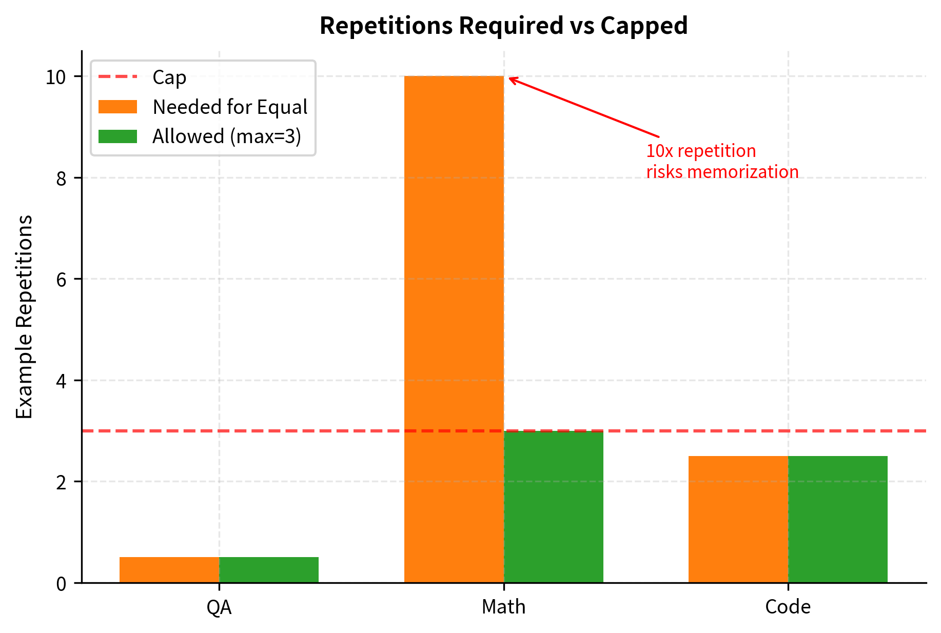
When training for multiple epochs, you must carefully manage how sampling and repetition interact. With proportional sampling across multiple epochs, the training process remains dominated by common tasks, potentially leading to severe underfitting on rare ones: after three epochs, the model may have seen each QA example three times while still struggling with math because those examples remain sparse in each epoch. Conversely, with equal sampling, rare task examples must be repeated far more frequently than common ones within each epoch to balance the distribution, and across multiple epochs this repetition compounds, dramatically increasing the risk of memorizing specific examples rather than learning general patterns.

To prevent this, you can cap how many times any single example appears during training:

The final dataset has 11,500 examples. The 'Math' task was capped at 3 repetitions to prevent overfitting. This balances task representation while avoiding memorization.

The key parameters for data mixing and sampling are:

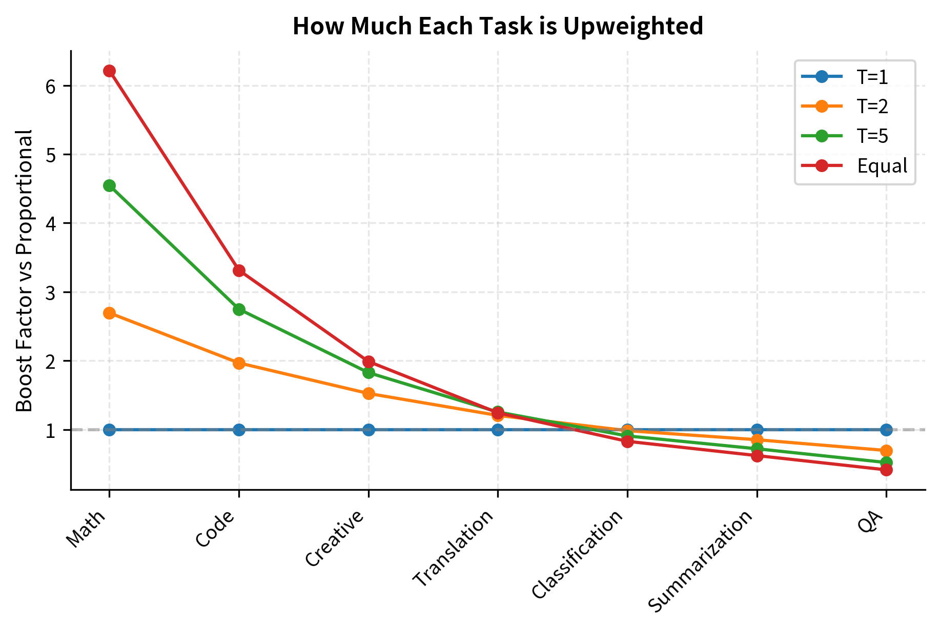
• temperature: Controls the sharpness of the sampling distribution. A higher temperature (e.g., $T=2$) upweights minority tasks compared to their natural frequency, ensuring they receive more training attention. Lower temperatures preserve more of the original distribution, while very high temperatures approach uniform sampling.
• max_repeats: The maximum number of times a single example can be repeated in a balanced dataset. This parameter prevents overfitting on small task categories by capping repetition even when equal sampling would require seeing those examples many more times.

Standard language modeling calculates loss for all tokens. In instruction tuning, this wastes capacity on reproducing instructions instead of learning to respond.

Consider an instruction tuning example:

Without loss masking, the model receives gradient updates for every token, including the instruction "Explain photosynthesis in simple terms." But reproducing user instructions is not the goal. The model should learn to generate helpful responses, not memorize prompts. Training on prompt tokens dilutes the learning signal with information the model already understands from pre-training.

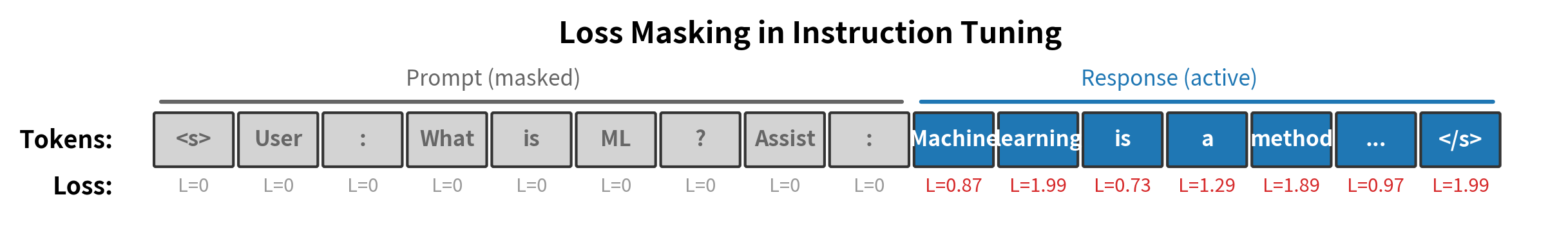
Loss masking addresses this by zeroing out the loss for prompt tokens. Only the assistant's response contributes to parameter updates:

The mask indicates which tokens should contribute to the loss. Typically, prompt tokens (system message and user input) receive a mask value of 0, while response tokens receive a mask value of 1.

Loss masks must align with tokenized sequences. This requires tracking where the prompt ends and the response begins:

The following visualization shows how loss masking focuses training on the response portion of each example:

Loss masking significantly affects what the model learns during instruction tuning. Without masking, gradients flow from both prompt and response tokens, diluting the signal that teaches response generation. With masking, all gradient information comes from response tokens, making training more efficient and focused.

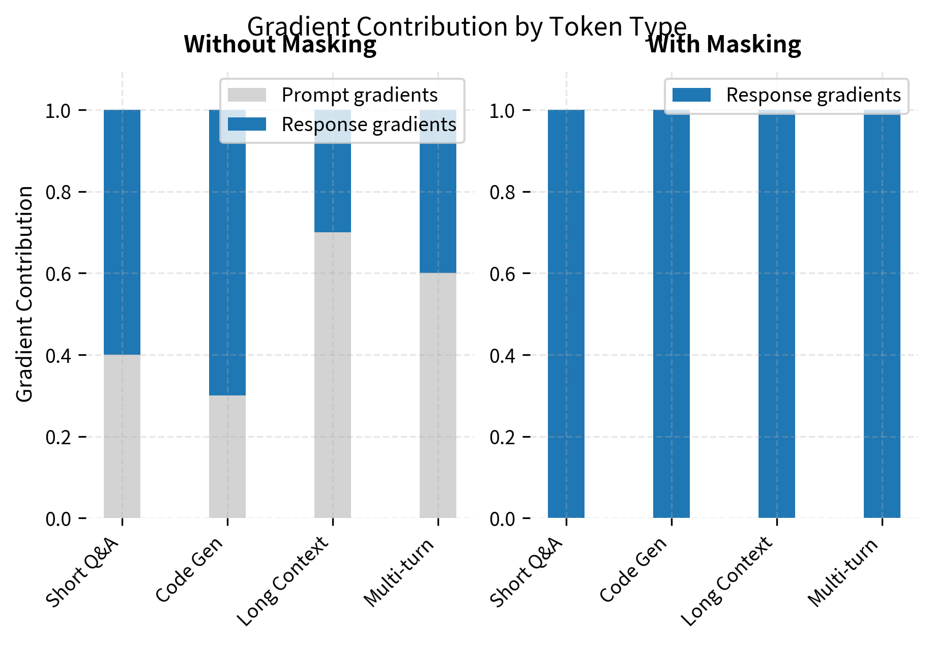
The effect is particularly pronounced in scenarios with long prompts relative to responses. In long-context applications or multi-turn conversations, prompts can comprise 60-70% of tokens. Without masking, most of the learning signal would be spent on reproducing context rather than learning to respond appropriately.

Instruction tuning requires careful hyperparameter selection. Unlike pre-training, which processes trillions of tokens over many epochs, instruction tuning typically involves much smaller datasets and fewer training steps. This concentrated training amplifies the importance of each hyperparameter choice.

The learning rate is typically lower than pre-training, usually in the range of $1 \times 10^{-5}$ to $5 \times 10^{-5}$. Higher learning rates risk catastrophic forgetting, where the model loses pre-trained capabilities while learning to follow instructions. Lower learning rates preserve more of the base model's knowledge but may require more training steps.

A warmup period helps stabilize early training. During warmup, the learning rate gradually increases from near-zero to the target value. This prevents large gradient updates before the model adapts to the new data distribution.

Larger batch sizes provide more stable gradient estimates but require more memory. Gradient accumulation allows effective large batches on limited hardware:

Effective batch sizes between 64 and 256 are common for instruction tuning. Smaller batches introduce more noise into gradient estimates, which can help generalization but may slow convergence. Larger batches converge faster but may generalize less well.

Instruction tuning typically uses 1-3 epochs over the training data. More epochs risk overfitting to the instruction format rather than learning general instruction-following capabilities. Signs of overfitting include:

• Training loss continues decreasing while validation loss increases
• Model outputs become formulaic or repetitive
• Performance degrades on held-out tasks

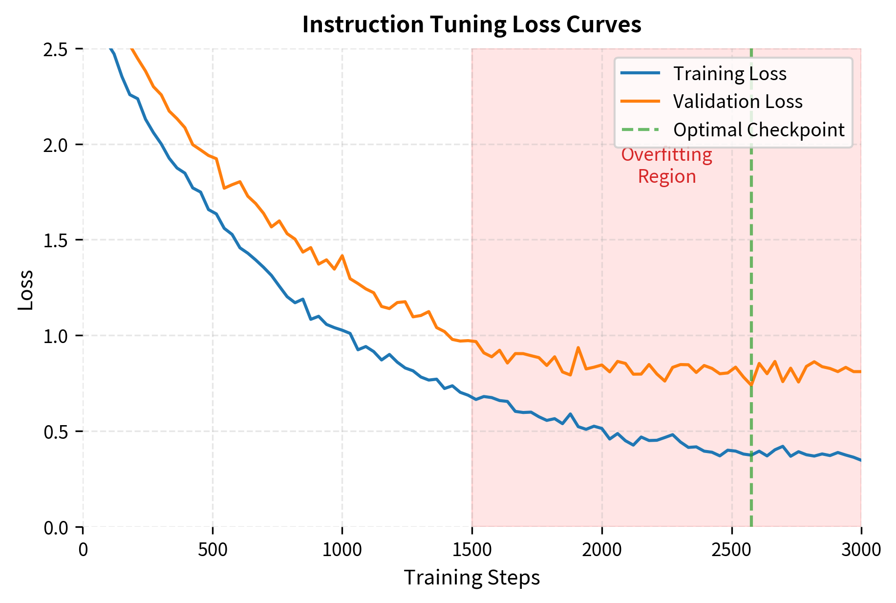
Early stopping based on validation loss helps prevent overfitting. Save checkpoints regularly and evaluate on held-out instruction examples to identify the optimal stopping point.

Instruction tuning naturally supports multi-task learning. By training on diverse instruction types simultaneously, the model learns transferable skills. A model trained on summarization, translation, and question-answering often performs better on each individual task than models trained separately, because the shared representations capture general language understanding.

The key benefits include:

• Positive transfer: Skills learned on one task improve performance on related tasks
• Regularization: Task diversity prevents overfitting to any single task pattern
• Emergent capabilities: Models sometimes gain abilities not explicitly trained, arising from the combination of skills

However, multi-task learning also introduces potential negative transfer when tasks conflict. For example, tasks requiring very different output styles (terse classification labels versus verbose explanations) may interfere with each other. Temperature-based sampling and careful task curation help mitigate these conflicts.

Instruction tuning training requires balancing multiple competing concerns: ensuring adequate coverage of minority tasks without overfitting, focusing learning on response generation through loss masking, and selecting hyperparameters that preserve pre-trained capabilities while teaching instruction following.

The key decisions covered in this chapter are:

1. Data mixing strategy: Use temperature-based sampling with $T \approx 2-3$ to balance task representation
2. Repetition capping: Limit how often small datasets are repeated to prevent memorization
3. Loss masking: Zero out loss on prompt tokens to focus learning on response generation
4. Hyperparameter selection: Use lower learning rates ($1-5 \times 10^{-5}$), moderate batch sizes (64-256), and few epochs (1-3) to avoid catastrophic forgetting

These techniques work together to produce models that follow instructions reliably while maintaining their broader language capabilities. The next chapter examines how to evaluate whether instruction tuning has succeeded.

Ready to test your understanding? Take this quick quiz to reinforce what you've learned about instruction tuning training.