Router Z-Loss: Numerical Stability for MoE Training

The auxiliary balancing loss we covered in the previous chapter addresses one necessary challenge in Mixture of Experts training: so tokens distribute evenly across experts. But MoE models face another subtle yet dangerous problem: router instability during training. As router logits grow unboundedly large, softmax computations become numerically unstable, gradients explode or vanish, and training can collapse entirely. Router z-loss provides an elegant solution by penalizing large router logits, keeping the gating network well-behaved throughout training. Z-loss is necessary for stable MoE training. The success of a training run often depends on this single auxiliary loss term.

Training large neural networks is already a fragile enterprise, but MoE architectures introduce a specific vulnerability that has nothing to do with the task itself. The router network sits at the center of every forward pass, deciding which experts process which tokens. If the router's computations become numerically ill-conditioned, every downstream expert receives garbage inputs, and the entire model can spiral into an unrecoverable failure state. Researchers at Google Brain first documented this failure mode systematically in the ST-MoE paper, where training runs on large MoE models would proceed smoothly for thousands of steps before suddenly crashing with NaN losses and exploding gradients. The culprit was always the same: logit magnitudes that had drifted far from the values needed for stable softmax computation.

Think of router logits as the "volume knobs" on a mixing board. If every knob is set to a moderate level, the audio output sounds reasonable and you can adjust individual knobs to change the mix. But if every knob has been gradually cranked up to maximum over hours of adjustments, the entire system saturates and you lose meaningful control. Z-loss is the mechanism that prevents all the knobs from being cranked up simultaneously, keeping them in a range where they remain useful and informative.

Understanding z-loss requires appreciating a subtle but important distinction: the routing decision and the logit magnitude are separate things. A router can make perfectly good routing decisions using logits like $[2.0, 0.5, 0.1]$ or using logits like $[20.0, 5.0, 1.0]$. In both cases, the router strongly prefers expert 1 and largely ignores experts 2 and 3. But the second set of logits creates exponential computations that strain floating-point arithmetic. Z-loss exploits this decoupling: it penalizes large magnitudes without penalizing the relative differences between logits that carry the actual routing information.

The point is that z-loss targets a specific mathematical quantity, the log-sum-exp of the logits, which is an elegant proxy for logit scale. This quantity has smooth gradients, approximates the maximum logit, and can be computed stably even when the logits themselves have already become extreme. By squaring this quantity and adding it to the training objective, we create a continuous pressure that counteracts the natural drift toward larger logit values throughout training. The result is a training run that remains numerically stable without sacrificing routing quality.

This chapter develops z-loss from first principles, starting with the root cause of router instability, working through the mathematical formulation and its gradient properties, and arriving at practical implementation guidance for combining z-loss with the load balancing loss from the previous chapter. We will also examine what goes wrong when z-loss is absent or improperly tuned, which illuminates why this seemingly simple regularization term has become a standard component of every serious MoE training recipe.

To understand why router instability occurs, we first need to revisit how routing decisions are made and why the underlying mathematics creates a hidden vulnerability. Recall from the discussion of gating networks that the router produces logits $z_i = W_r h_i$ for each input token $h_i$, where $W_r$ is the router weight matrix. These logits represent the raw, unnormalized scores that indicate how strongly the router prefers each expert for a given token. These logits pass through a softmax to produce routing probabilities:

where:

• $p_j$: the probability assigned to expert $j$
• $z_j$: the router logit for expert $j$
• $N$: the total number of experts
• $\exp(z_j)$: the exponential of the logit, so a positive value
• $\sum_{k=1}^{N} \exp(z_k)$: the sum over all $N$ experts, serving as the normalization constant

The softmax function turns arbitrary real-valued logits into a proper probability distribution where all values are positive and sum to one. This transformation is elegant and widely used, but it introduces subtle numerical challenges when the input logits span extreme ranges.

During training, nothing explicitly constrains the magnitude of these logits. The neural network is free to produce logits of any size, and the gradient descent process will adjust parameters in whatever direction minimizes the loss function. The softmax function is scale-invariant in its output probabilities: multiplying all logits by a constant doesn't change the relative probabilities. If you double all the logits, you still get the same ranking and the same probability assignments. However, scale dramatically affects the sharpness of the distribution and the numerical stability of the computation. This simple property creates a hidden danger that only appears as training progresses.

It is worth pausing on this scale-invariance property because it has important consequences. The router's job, from a functional perspective, is to rank experts and select the best ones. Rankings are fully determined by the relative order of logits, not their absolute values. Yet the training loss is sensitive to the absolute values through the softmax computation and its gradients. This mismatch between what the router needs (relative ranking) and what the optimization process adjusts (absolute values) creates the conditions for unconstrained logit growth.

As training progresses, the router learns to route tokens to appropriate experts by increasing the logits for preferred experts relative to others. This is exactly what we want: the router should learn to distinguish which expert is best suited for each type of input. Without constraints, however, this creates a natural logit drift toward larger logit magnitudes. If expert 3 is consistently preferred for certain tokens, the router learns to make $z_3$ large and positive while other logits become large and negative. The optimization process finds that making these differences more extreme leads to more confident routing decisions.

This drift accelerates over time through a self-reinforcing feedback loop. Larger logits create sharper probability distributions, which produce stronger gradients for the "winning" experts. When the probability assigned to the chosen expert approaches 1.0, the gradient signal becomes very clear: this expert should handle this token. These stronger gradients further increase the logit gap, which creates even sharper distributions, which produce even stronger gradients. This positive feedback loop pushes logits toward extreme values without any natural stopping point.

To illustrate this phenomenon concretely, consider a router that starts with logits around $[1.0, 0.8, 0.5, 0.2]$. The corresponding probabilities might be roughly $[0.35, 0.29, 0.21, 0.15]$, which is a reasonably soft distribution. After many training steps, if expert 1 is consistently correct, the logits might evolve to $[10.0, 3.0, 2.0, 1.0]$, giving probabilities closer to $[0.99, 0.009, 0.0003, 0.0001]$. The training process has learned to be more confident, but the logit magnitudes have increased dramatically. Left unchecked, this drift continues until logits reach values that cause computational problems.

Think of logit drift as a ratchet mechanism: each training step tightens the routing distribution slightly, and there is no counter-pressure to loosen it. Every time the model correctly identifies an expert assignment, the gradient pushes the logits further apart, reinforcing the decision. The model is rewarded for confidence and responds by becoming ever more confident, regardless of whether the extra confidence improves task performance. The problem is unbounded confidence that eventually strains numerical computations.

Large logits cause several numerical problems that can derail training entirely. These issues show why z-loss targets logit magnitudes:

• Softmax overflow: Computing $\exp(z_j)$ for $z_j > 709$ (float64) or $z_j > 88$ (float32) produces infinity. When any exponential term overflows, the entire softmax computation becomes undefined. Even a single overflowed value corrupts the probability calculation for all experts.

• Softmax underflow: Computing $\exp(z_j)$ for very negative $z_j$ produces zero due to floating-point underflow. This might seem harmless since small probabilities should be near zero anyway. However, when combined with division operations, these zeros can cause division-by-zero errors or produce undefined gradients.

• Gradient instability: The softmax gradient involves terms like $p_j(1 - p_j)$, which vanishes as probabilities approach 0 or 1. When the router becomes extremely confident, assigning probability 0.9999 to one expert and 0.0001 to others, the gradients become tiny. This gradient saturation prevents the router from learning to change its routing decisions even when it should.

• Loss of precision: When logits span a huge range, floating-point arithmetic loses significant digits. A computation involving $\exp(50)$ and $\exp(-50)$ cannot represent both values accurately in the same calculation, even with double precision. This precision loss introduces numerical noise that accumulates over training steps.

While the softmax-with-max-subtraction trick (subtracting $\max_j z_j$ before exponentiation) prevents overflow in the forward pass, it does not address the instability that large logit magnitudes create for gradient flow. The backward pass still suffers from saturated gradients and precision issues. The max-subtraction trick only helps with the exponential computation; it does not prevent the underlying logit drift that causes these problems. Z-loss addresses this root cause rather than individual symptoms.

The basic issue is that the max-subtraction trick is a computational workaround, not a solution to the underlying problem. You can stably compute $\text{softmax}([1000, 999, 998])$ using max-subtraction: subtract 1000 from all values, then compute $\text{softmax}([0, -1, -2])$. But the gradient of this softmax with respect to the original logits is still nearly zero, because the probabilities are $[0.731, 0.269, 0.099]$, and the gradient involves these probabilities directly. The router has essentially made a near-deterministic decision, and near-deterministic decisions have tiny gradients. Max-subtraction makes the computation numerically stable without which makes it informationally useful.

Router instability typically manifests in several recognizable ways that you should monitor:

1. Training loss spikes: Sudden, unexpected increases in loss occur as numerical issues cascade through the network. The loss might be decreasing smoothly for thousands of steps, then suddenly jump to a much higher value or even become NaN. These spikes often indicate that router logits have grown large enough to cause computational problems.

2. Gradient explosions: NaN or inf values appearing in gradients signal that the numerical instability has propagated to the backward pass. Once gradients contain invalid values, parameter updates become meaningless, and the model parameters can become corrupted. Recovering from gradient explosions often requires rolling back to an earlier checkpoint.

3. Expert collapse: The router becoming stuck on a single expert due to saturated gradients represents a subtle but serious failure mode. When logits become extreme, the router cannot learn to route tokens to different experts even when the current routing is suboptimal. The gradients for non-selected experts become vanishingly small, freezing the routing pattern in place.

4. Poor generalization: Overconfident routing that doesn't transfer to new inputs indicates that the model has memorized routing patterns rather than learning generalizable features. When the router makes extremely sharp decisions based on subtle input features, small changes in input distribution can completely change routing behavior in unpredictable ways.

These issues become more severe as model scale increases. Larger models have more parameters in the router network, more capacity to push logits to extreme values, and longer training runs that provide more opportunity for drift to accumulate. The ST-MoE paper from Google observed that without z-loss, larger MoE models frequently experienced training instabilities that smaller models avoided. This scale-dependent behavior makes z-loss increasingly important as the field moves toward ever-larger MoE architectures.

These failures often appear suddenly after training seems to be going well. A common failure pattern is a long period of healthy, decreasing loss followed by an abrupt instability that wipes out gains from thousands of training steps. Logit drift is slow and cumulative: logits grow gradually over many batches, but the numerical consequences trigger only when they exceed specific thresholds. This makes preventive regularization, like z-loss, more effective than reactive measures such as checkpoint rollback.

Router z-loss directly penalizes large logit magnitudes by adding a regularization term to the training objective. Rather than placing hard constraints on logit values, which would require constrained optimization techniques, z-loss uses soft regularization that integrates smoothly with standard gradient descent. The formulation targets the log-sum-exp of router logits, a smooth, differentiable proxy for the maximum logit that has particularly nice mathematical properties.

The design of z-loss reflects several important engineering considerations. Hard constraints like "no logit may exceed value X" are difficult to enforce efficiently in distributed training and create discontinuous gradients at the constraint boundary. Penalty terms on individual logits (such as L2 regularization) apply pressure uniformly, which can interfere with the router's ability to develop discriminative patterns. Z-loss avoids both problems: it is smooth, it automatically focuses pressure on the largest logits, and it is trivial to compute alongside the standard softmax.

Think of z-loss as a built-in pressure release valve. As logits grow, the penalty grows even faster (quadratically), creating an increasing counterforce that slows the drift before it causes problems. This is analogous to a thermostatic system: when the temperature rises above a comfortable level, the cooling mechanism kicks in harder, establishing a stable equilibrium rather than letting unbounded temperature increase.

Router z-loss directly penalizes large logit magnitudes by adding a regularization term to the training objective. Rather than placing hard constraints on logit values, which would require constrained optimization techniques, z-loss uses soft regularization that integrates smoothly with standard gradient descent. The formulation targets the log-sum-exp of router logits, a smooth, differentiable proxy for the maximum logit that has particularly nice mathematical properties.

For a batch of $B$ tokens, where token $i$ has router logits $z_{i,j}$ for expert $j$, the z-loss is defined as:

where:

• $\mathcal{L}_z$: the router z-loss
• $B$: the batch size (number of tokens)
• $N$: the number of experts
• $z_{i,j}$: the logit for token $i$ and expert $j$
• $\log \sum \ldots$: the log-sum-exp term approximating the maximum logit

Let's unpack this formula to understand how it works. The innermost part, $\sum_{j=1}^{N} \exp(z_{i,j})$, computes the sum of exponentials of all logits for a single token. This sum is exactly the normalization constant that appears in the denominator of the softmax function. Taking the logarithm of this sum gives us the log-sum-exp (LSE), which has a natural interpretation as a "soft maximum" of the logits.

The inner term $\log \sum_j \exp(z_{i,j})$ is the log-sum-exp (LSE) of the logits for token $i$. This function has a useful property that makes it ideal for our purposes: it approximates the maximum logit while remaining smooth and differentiable everywhere:

where:

• $\max_j z_{i,j}$: the largest logit value for token $i$, representing the router's most confident assignment
• $N$: the total number of experts in the layer
• $\log N$: a constant upper bound on the approximation error, roughly 2.1 for 8 experts or 4.2 for 64 experts

Why does this formula make sense? Notice that when one logit $z_{i,k}$ dominates all others by a large margin, $\sum_j \exp(z_{i,j}) \approx \exp(z_{i,k})$, so $\log \sum_j \exp(z_{i,j}) \approx z_{i,k} = \max_j z_{i,j}$. The approximation is tight when the routing is confident. When all logits are equal, the sum is $N \cdot \exp(z)$ and the log-sum-exp equals $z + \log N$, which is exactly $\log N$ above the maximum. So the bound holds with equality at both extremes.

This inequality tells us that the LSE always lies between the maximum logit and the maximum logit plus $\log N$. For typical expert counts (8, 16, or 64 experts), $\log N$ is a small constant (approximately 2.1, 2.8, or 4.2 respectively), so the LSE closely tracks the maximum logit. However, unlike the hard maximum function, which has discontinuous gradients at points where multiple logits are tied, the LSE is smooth everywhere. This smoothness is important for gradient-based optimization.

Squaring this quantity and averaging across tokens creates a penalty that grows quadratically as logits increase. The squaring operation has two important effects: it ensures the loss is always non-negative, and it provides increasingly strong regularization as logits grow. A token with LSE value of 10 contributes 100 to the loss, while a token with LSE value of 20 contributes 400. This quadratic growth creates strong pressure to keep logits bounded without overly penalizing moderate values.

The log-sum-exp formulation has several advantages over alternative approaches to constraining logit magnitudes. These advantages show why this design has become standard in MoE training rather than simpler alternatives:

• Smooth gradients: Unlike penalties on $\max_j z_j$ (which has discontinuous gradients at points where the maximum switches from one logit to another) or $\sum_j z_j^2$ (which penalizes all logits equally regardless of their relative magnitudes), LSE smoothly emphasizes the largest logits while giving gradients to all experts. When one logit is much larger than the others, the LSE gradient is concentrated on that logit. When multiple logits are similar, the gradient is distributed among them. This smooth interpolation between these cases makes optimization well-behaved and prevents the abrupt gradient changes that occur with hard maximum penalties.

• Scale awareness: The LSE naturally captures the "effective scale" of the logit distribution in a way that considers both the maximum value and the spread. For example, a distribution with logits $[10, 10, 10]$ has an LSE of approximately $11.1$, while a distribution with logits $[30, 30, 30]$ has an LSE of approximately $31.1$. Although both produce identical uniform probability distributions (and thus have the same entropy), their LSE values differ significantly, correctly which reflects that the larger logits pose greater stability risks. This is precisely the behavior we want: penalizing scale independently of routing patterns.

• Numerical stability: The LSE is itself computed stably using the max-subtraction trick, avoiding the very overflow issues we are trying to prevent. Modern deep learning frameworks implement numerically stable versions of log-sum-exp that never overflow, making z-loss reliable to compute even when logits have already drifted to large values. This means z-loss can be applied as a corrective measure even when training has already started experiencing instability.

• Computational efficiency: The LSE is already computed as an intermediate result during the softmax calculation. In practice, the numerator $\sum_j \exp(z_{i,j})$ appears in the softmax denominator, and the LSE is just the log of this quantity. Frameworks like PyTorch's torch.logsumexp implement this without additional overhead, making z-loss essentially free to compute in terms of wall-clock time.

An alternative approach one might consider is simply applying L2 regularization directly to the router weights $W_r$. This would prevent the weights from growing large, which would indirectly bound logit magnitudes. The problem with this approach is that weight decay applies pressure uniformly to all router weights, including those that are small and produce benign logits. Z-loss, by contrast, applies pressure specifically proportional to the current logit magnitudes, putting correction where it is most needed while leaving well-behaved logits largely undisturbed.

To understand the effect of z-loss on training dynamics, we derive its gradient with respect to the router logit $z_{i,j}$. This derivation reveals how the loss creates corrective pressure on large logits and why the pressure is proportional to both the current scale and the routing confidence.

The gradient we want to compute answers the question: if logit $z_{i,j}$ increases by a small amount, how does the z-loss change? A large gradient means z-loss strongly penalizes further increases in this logit. This provides a restoring force. A small gradient means z-loss is nearly indifferent to this logit. This allows it to change freely.

Applying the chain rule to the squared term:

where:

• $\frac{\partial \mathcal{L}_z}{\partial z_{i,j}}$: the gradient of the loss with respect to a specific logit
• $B$: the batch size
• $\text{LSE}(z_i)$: the log-sum-exp value for token $i$
• $\text{softmax}(z_i)_j$: the probability assigned to expert $j$

The key insight in this derivation is that the derivative of the log-sum-exp with respect to one of its inputs is exactly the corresponding softmax probability. This elegant relationship emerges from the structure of the exponential function and is a standard result in mathematical statistics. Formally, if $\text{LSE}(z) = \log \sum_j \exp(z_j)$, then $\frac{\partial \text{LSE}}{\partial z_j} = \frac{\exp(z_j)}{\sum_k \exp(z_k)} = \text{softmax}(z)_j$.

Why does this formula make sense? Notice that the gradient has exactly two factors multiplied together: the current LSE value (representing the "scale emergency severity") and the softmax probability (representing "which logit is most responsible for the high scale"). The product naturally directs corrective pressure where it is most needed. When the LSE is small, the gradient is small, meaning z-loss barely touches the router when logits are healthy. When the LSE grows large, the gradient scales up proportionally. This provides increasingly aggressive correction. This self-calibrating behavior is what makes z-loss an effective regularizer rather than a blunt instrument.

This gradient formula reveals important behavior that explains why z-loss is effective:

• The gradient is proportional to the current softmax probability: experts receiving more routing get larger gradients pushing their logits down. This is exactly what we want, as the experts with the largest logits (and therefore highest probabilities) receive the strongest corrective signal. Experts that are already receiving little routing probability receive only small gradients from z-loss, letting them to remain available for future routing without being artificially suppressed.

• The gradient scales with the current LSE value: larger logits create stronger corrective pressure. When the LSE is small (showing well-behaved logits), the z-loss gradient is correspondingly small and doesn't interfere much with task learning. When the LSE grows large (showing potential instability), the gradient grows proportionally, creating a stronger restoring force.

• The quadratic nature (from squaring) provides increasingly strong regularization as logits grow. The factor of 2 from the power rule, combined with the LSE scaling, means the gradient grows faster than linearly with logit magnitude. This provides gentle regularization for moderate logits but strong correction for extreme values, striking a balance between letting useful routing patterns and preventing numerical instability.

To make the mathematics concrete, let's trace through a single z-loss computation with specific numbers. Suppose we have a batch of $B = 3$ tokens and $N = 4$ experts. The router produces the following logit matrix:

where row $i$ contains the logits for token $i$ across all four experts. Notice that token 1 has moderate, nearly uniform logits, while token 3 has a very large logit for expert 1.

Step 1: Compute LSE for each token.

For token 1, with logits $[3.0, 1.0, 0.5, -0.5]$:

For token 2, with logits $[1.5, 1.2, 1.0, 0.8]$:

For token 3, with logits $[8.0, 2.0, 1.0, 0.0]$:

Notice that token 3's LSE is almost exactly equal to its maximum logit (8.0), confirming the approximation is tight when one logit dominates strongly. Token 2's LSE is 2.55, compared to its maximum logit of 1.5, a gap of 1.05, close to $\log(4) \approx 1.39$ since the logits are nearly equal.

Step 2: Square each LSE value.

Step 3: Average across the batch.

Step 4: Understand what this tells us.

Token 3 contributes 64.00 to the sum, while tokens 1 and 2 together contribute only 16.87. Token 3's extreme logit of 8.0 for expert 1 is responsible for nearly 80% of the total z-loss, even though it is only one of three tokens. This is the quadratic amplification working as intended: logit values that are dangerously large receive a disproportionate share of the penalty, creating strong corrective pressure exactly where it is most needed.

Step 5: Compute the gradient for the dominant logit.

For token 3, the softmax probability for expert 1 is approximately:

The z-loss gradient for this logit is:

This is a substantial gradient that will push $z_{3,1}$ downward in the next parameter update, counteracting the logit drift that produced this large value. The other logits for token 3 receive much smaller gradients, proportional to their much smaller softmax probabilities. This numerical trace confirms the theoretical properties we derived: the corrective pressure is both scale-proportional and routing-probability-weighted.

Z-loss addresses router instability through several complementary mechanisms that work together to maintain training stability. These mechanisms explain why this regularization works when simpler alternatives fall short.

By continuously penalizing large LSE values, z-loss creates a restoring force that counteracts the natural drift toward larger logits. Whenever logits grow too large, the z-loss gradient pushes them back down. This establishes an equilibrium where the router learns discriminative logit patterns without unbounded growth. The router can still learn to prefer certain experts for certain inputs, but the absolute magnitude of the preferences remains bounded.

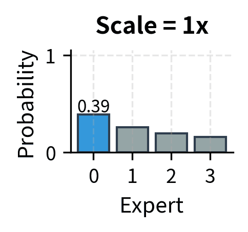
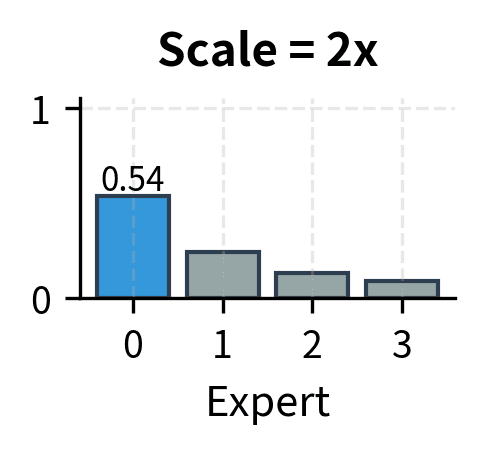
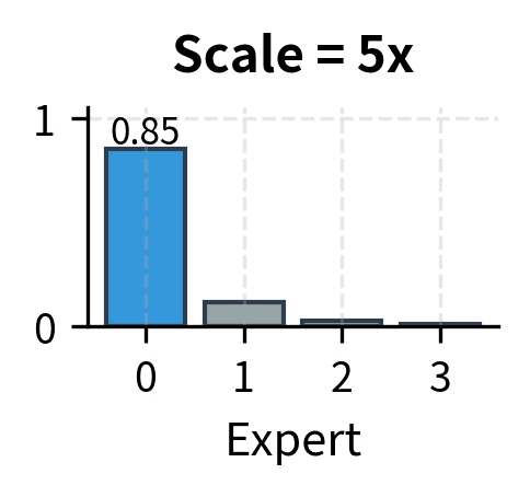
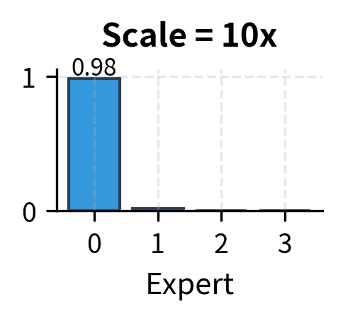
The key insight is that useful routing doesn't require extreme logits. A router with logits $[2.0, 0.5, 0.3, 0.1]$ can effectively route to expert 1 with probability approximately 0.54, which is sufficient to ensure expert 1 is selected in top-2 routing. Increasing these to $[20.0, 5.0, 3.0, 1.0]$ makes the probability approximately 0.999999, but this extreme confidence adds no practical benefit while creating numerical hazards. The routing decision is the same in both cases, but the numerical properties are vastly different. Z-loss exploits this redundancy by penalizing magnitude while leaving routing patterns intact.

This equilibrium behavior is similar to other regularization techniques like weight decay, which creates restoring forces that prevent unbounded parameter growth. The difference is that z-loss specifically targets the router logits, which are the quantities most directly responsible for numerical stability in MoE training. Weight decay on the router's weight matrix would also bound logit magnitudes indirectly, but z-loss provides a more direct and interpretable constraint on the actual quantities causing instability.

Z-loss implicitly encourages a "softer" probability distribution over experts, as if the softmax were computed at a higher temperature. By penalizing the logit scale, it prevents the extremely peaked distributions that arise from large logit differences. When logit differences are bounded, the resulting probability distributions maintain non-trivial probabilities for multiple experts rather than putting all probability mass on a single expert.

Think of softmax temperature as a dial controlling how decisive the router is allowed to be. High temperature means the router is uncertain and distributes probability across many experts. Low temperature means the router is highly confident and concentrates probability on one expert. Z-loss effectively sets a lower bound on the temperature by preventing logit magnitudes from growing too large, even though it doesn't directly manipulate the temperature parameter.

This softer routing has several benefits that extend beyond mere numerical stability:

• Better gradient flow: Non-zero probabilities for multiple experts mean gradients flow to more expert parameters during each training step. Even experts that aren't selected still receive gradient signals through the softmax probabilities, letting them to continue learning and remain competitive. This prevents the "rich get richer" dynamic where selected experts improve while others stagnate.

• Improved exploration: The router remains willing to try alternative experts rather than fixating on past choices. Soft probabilities mean that stochastic routing (if used) can occasionally select non-preferred experts, letting the model to discover better routing patterns. Even with deterministic top-k routing, softer probabilities mean the router can more easily shift its preferences as the experts evolve during training.

• Smoother learning: Gradual probability shifts rather than sudden expert switches create more stable training dynamics. When routing probabilities can change continuously rather than jumping between extremes, the experts experience more consistent training signals. This consistency helps experts develop coherent specializations rather than being whipsawed by sudden changes in their token assignments.

Beyond stability, z-loss regularizes routing and can improve generalization to new data. By preventing overconfident routing, it encourages the model to develop routing patterns based on reliable input features rather than spurious correlations or memorized associations. The regularization effect is similar to adding noise or using dropout, both of which prevent overconfident predictions.

Models trained with z-loss often show better performance on held-out data, particularly for inputs that differ from training distributions. When the router is forced to maintain some uncertainty in its routing decisions, it learns to base those decisions on stable, generalizable features rather than memorizing specific training examples. This improved generalization is especially valuable in language models, which must handle diverse inputs that may differ substantially from training data.

The regularization benefit of z-loss complements the stability benefit: both arise from the same mechanism of preventing extreme logit values, but they manifest in different ways. Stability is visible during training as the absence of loss spikes and gradient explosions. Regularization is visible during evaluation as improved performance on out-of-distribution inputs. The fact that a single simple regularization term achieves both goals simultaneously is part of what makes z-loss so valuable in practice.

One way to understand the generalization benefit is through routing stability. A model with extreme logits will route a token to exactly one expert with near-certainty, based on whatever features the router has learned to use. If those features happen to be noisy or domain-specific, routing on test data may look completely different from training data. A model with bounded logits maintains some probability mass on multiple experts. This provides a routing ensemble that is more reliable under distribution shift.

The z-loss coefficient $\alpha_z$ controls the strength of logit regularization and represents the primary hyperparameter that you must tune when using this technique. Before choosing a value, it helps to understand the mathematical relationship between the coefficient and the equilibrium logit magnitude. In equilibrium, the z-loss gradient equals the gradient from other terms pushing logits up, which means that larger coefficients correspond to smaller equilibrium logit values.

The z-loss coefficient $\alpha_z$ controls the strength of logit regularization and represents the primary hyperparameter that you must tune when using this technique. The total training objective with z-loss takes the form:

where:

• $\mathcal{L}_{\text{total}}$: the combined training objective that guides all parameter updates
• $\mathcal{L}_{\text{task}}$: the primary task loss (cross-entropy for language modeling)
• $\alpha_z$: the z-loss weighting coefficient, determining how strongly logit magnitude is penalized
• $\mathcal{L}_z$: the auxiliary z-loss term defined in the previous section

Choosing an appropriate coefficient requires balancing stability against routing effectiveness. Too small a coefficient provides insufficient regularization and allows instability. Too large a coefficient over-regularizes the router, preventing it from learning sharp routing patterns that enable expert specialization. The optimal coefficient lies in a middle ground that must be found empirically for each setting, though some general guidelines narrow the search considerably.

The task loss and z-loss operate on different scales. A typical cross-entropy task loss might be in the range of 3-8 during language model training (corresponding to perplexity values of 20-3000). A typical z-loss value might be 4-16 for well-behaved logits (corresponding to LSE values of 2-4). Setting $\alpha_z = 10^{-3}$ means the z-loss contributes roughly 0.004-0.016 to the total objective, a small fraction of the task loss. This relative scaling is intentional: z-loss should be a minor influence on the training objective, nudging the router toward stability without dominating the optimization.

Typical z-loss coefficients fall in the range $10^{-4}$ to $10^{-2}$, with several factors influencing the optimal choice:

• Model scale: Larger models often need stronger z-loss (higher $\alpha_z$) because they have more capacity for logit growth. The router network in a large model has more parameters and processes higher-dimensional representations, giving it more "room" to develop extreme logit patterns. The longer training runs typical of larger models also provide more time for drift to accumulate.

• Number of experts: More experts slightly increase the LSE for a given max logit because of the $\log N$ term in the LSE bounds, so the coefficient may need adjustment. However, this effect is typically small compared to other factors, since $\log N$ grows slowly with the number of experts.

• Training stability requirements: If training instabilities occur despite using z-loss, increasing $\alpha_z$ by 2-5x often helps stabilize training. This is a common first response to observed instability. However, if instabilities persist even with high z-loss coefficients, other factors like learning rate or batch size may need adjustment.

• Routing sharpness: Very high $\alpha_z$ can make routing too soft, reducing the benefit of expert specialization. When routing becomes nearly uniform, different experts receive similar token mixtures, preventing them from developing distinct specializations. Monitoring expert utilization and specialization can reveal if the z-loss coefficient is too high.

The ST-MoE paper used $\alpha_z = 10^{-4}$ as a starting point, finding it sufficient to stabilize training while preserving routing quality. This value has become a common default in subsequent MoE implementations, though you should treat it as a starting point rather than a universal optimum.

A practical approach to setting the z-loss coefficient involves the following steps, which balance systematic exploration with responsive adjustment:

1. Start conservative: Begin with $\alpha_z = 10^{-4}$ and monitor training stability. This conservative starting point provides some regularization without being so strong that it prevents useful routing patterns from developing. Most training runs will be stable at this coefficient.

2. Track LSE statistics: Log the mean and max LSE values across training batches. Healthy values typically stay below 10, though this depends on the number of experts. If LSE values grow steadily throughout training, the z-loss coefficient may need to be increased. If LSE values drop quickly to very small values, the coefficient may be too high.

3. Watch for instability: If loss spikes or NaN gradients occur, increase $\alpha_z$ by 2-5x. These events indicate that the current regularization strength is insufficient to prevent numerical problems. After increasing the coefficient, training may need to restart from an earlier checkpoint before the instability occurred.

4. Check routing quality: If routing becomes too uniform (all experts receiving similar load), reduce $\alpha_z$. Uniform routing defeats the purpose of having multiple experts, since all experts would receive the same training signal and develop similar capabilities. Some variation in expert load is healthy and indicates that the router is learning useful distinctions.

5. Validate on held-out data: Ensure z-loss isn't hurting generalization through over-regularization. While z-loss typically improves generalization by preventing overconfident routing, excessively strong regularization could prevent the model from learning useful routing patterns altogether.

In practice, many production MoE training setups monitor both LSE statistics and routing entropy simultaneously, using them as complementary diagnostics. LSE statistics reveal whether logit magnitudes are creeping up, while routing entropy reveals whether the routing distribution is becoming too uniform or too peaked. Both metrics should stabilize at healthy values during a well-tuned training run.

Some implementations use dynamic z-loss coefficients that change during training, adapting the regularization strength to the needs of different training phases:

• Warmup: Start with higher $\alpha_z$ during early training when instabilities are most common, then reduce as training stabilizes. Early training often sees rapid parameter changes that can push logits to extreme values, making strong regularization especially valuable. As training converges and parameters change more slowly, weaker regularization allows sharper routing.

• Curriculum: Increase $\alpha_z$ as model scale grows during progressive training. Some training approaches start with a small model and gradually increase its size. As the model grows, the capacity for logit drift increases, motivating stronger regularization.

• Adaptive: Adjust $\alpha_z$ based on observed LSE statistics, increasing when values exceed a threshold and decreasing when values are safely bounded. This approach automatically responds to the actual training dynamics rather than following a predetermined schedule. The risk is that adaptive schedules can be difficult to debug if they behave unexpectedly.

Dynamic schedules add implementation complexity but can improve training efficiency by applying strong regularization only when and where it is needed. For most practical purposes, a fixed coefficient tuned carefully at the start of training works well. Dynamic schedules become more valuable in very long training runs where the optimal regularization strength may change over time.

Real MoE systems use both load balancing loss (from the previous chapter) and z-loss together. These losses address complementary problems and work synergistically to create stable, effective MoE training. Neither loss alone is sufficient: load balancing without z-loss can still experience numerical instability, while z-loss without load balancing allows expert collapse and utilization imbalance.

These two problems are separate. Load balancing addresses a resource-allocation question: are all experts being used effectively? Z-loss addresses a computational-stability question: are the router's computations numerically well behaved? A model could theoretically have perfectly balanced expert load while still experiencing numerical instability in the router computation. Conversely, a model could have numerically stable logits while all routing probability concentrates on a single expert. Solving one problem does not solve the other, which is why both losses are included in the training objective.

Think of load balancing and z-loss as two different maintenance tasks for the same machinery. Load balancing is like making sure all the machinery components are getting equal use, preventing any single component from wearing out while others sit idle. Z-loss is like making sure the machinery is operating within safe temperature and pressure ranges. You need both: balanced use prevents premature failure of individual components, while operating within safe ranges prevents the entire system from breaking down.

The complete MoE training objective combines the task loss with both auxiliary losses:

where:

• $\mathcal{L}_{\text{total}}$: the complete joint objective
• $\mathcal{L}_{\text{task}}$: the primary task loss
• $\mathcal{L}_{\text{aux}}$: the auxiliary balancing loss (encourages uniform expert utilization)
• $\mathcal{L}_z$: the z-loss (prevents logit instability)
• $\alpha_{\text{aux}}, \alpha_z$: weighting coefficients for the auxiliary terms

This combined objective guides the model toward three goals simultaneously: achieving good task performance, maintaining balanced expert utilization, and preserving numerical stability. The relative importance of these goals is controlled by the two auxiliary coefficients.

Why does this formula make sense? Notice that the task loss operates at the macro scale of model performance, typically measured in nats or bits. The auxiliary losses operate at the micro scale of routing behavior. The coefficients $\alpha_{\text{aux}}$ and $\alpha_z$ serve as unit conversion factors, adjusting the scale of each auxiliary loss to make it numerically comparable to the task loss gradient. Without appropriate coefficients, one term could completely dominate the gradient, preventing the other terms from having any effect.

The two auxiliary losses serve distinct purposes that together create a reliable training framework:

Load balancing loss ensures that all experts are used and that no expert becomes overloaded or underutilized. Z-loss ensures that the routing computation itself remains numerically stable. These concerns are orthogonal: a model could have perfectly balanced load with numerically unstable logits, or stable logits with highly imbalanced load. Both auxiliary losses are needed to achieve both goals.

Understanding this orthogonality also clarifies when to increase each coefficient. If you observe expert imbalance (some experts receiving too many or too few tokens), increase $\alpha_{\text{aux}}$. If you observe training instability (loss spikes, NaN values, or LSE growth), increase $\alpha_z$. The two problems have distinct diagnostic signatures and distinct remedies, which makes them tractable to address independently.

The two losses can interact in subtle ways that you should understand:

• Synergy: Z-loss keeps routing soft, which makes it easier for load balancing to spread tokens across experts. Hard routing with very peaked probabilities resists load balancing pressure because the gradient from load balancing loss is proportional to softmax probabilities. When probabilities are nearly binary (0.99 for one expert, 0.01 for others), the load balancing gradient can only adjust the dominant expert's logit. Softer probabilities distribute the gradient across all experts, making load balancing more effective.

• Tension: Very strong z-loss ($\alpha_z$ too high) can make routing nearly uniform, reducing the importance of load balancing. When z-loss forces all logits to be similar, the resulting routing probabilities are already close to uniform regardless of load balancing. In this regime, further increasing load balancing coefficient has little effect. Conversely, aggressive load balancing might push some expert logits up to attract more tokens, which increases z-loss.

• Balance: Finding the right coefficient combination requires considering both effects. A common starting point is $\alpha_{\text{aux}} = 10^{-2}$ and $\alpha_z = 10^{-4}$, making load balancing the stronger constraint with z-loss giving background stabilization. This ratio reflects the fact that expert imbalance is typically a more pressing problem than numerical instability in early training, though both must be controlled.

The interaction between these losses also has an indirect effect on the experts themselves. When load balancing maintains reasonable utilization and z-loss maintains soft routing, the experts receive diverse training signals from many different token types. This diversity is what allows each expert to develop a distinct specialization over the course of training. Without these regularization terms working together, experts either collapse to handling everything (with no specialization) or become so specialized that they are useless for the full distribution of inputs.

Let's implement z-loss and observe its effect on router behavior. We'll build on the MoE infrastructure from previous chapters.

The core z-loss computation follows directly from the mathematical definition. The implementation is simple precisely because PyTorch's logsumexp function handles the numerically stable computation internally, applying the max-subtraction trick automatically.

Now let's create a router class that computes both routing probabilities and the z-loss. The key design principle is to compute z-loss on the raw logits, before any softmax or top-k selection. Computing z-loss after softmax would be mathematically incorrect, as the softmax output is already a probability distribution bounded between 0 and 1, which cannot exhibit the logit drift we are trying to prevent.

Let's visualize how z-loss affects logit distributions during training. The simulation below introduces a "task loss" that deliberately encourages larger logit magnitudes, mimicking the natural logit drift that occurs in real MoE training. We then compare training runs with different z-loss coefficients to see how the regularization contains this drift.

Without z-loss, the logit magnitudes grow freely. With z-loss applied, the optimizer continuously pushes logits back toward smaller values, establishing a stable equilibrium. The strength of the equilibrium is controlled by the coefficient: a larger coefficient produces a lower equilibrium logit magnitude, at the cost of potentially over-constraining the router.

Let's implement a complete MoE layer that computes both load balancing and z-loss. This implementation mirrors what you would find in production MoE systems, combining the two auxiliary loss terms in a single forward pass.

The model processes the input shape [4, 16, 128] and produces a matching output shape, confirming that the MoE layer is dimensionality-preserving. The auxiliary losses are non-zero, showing that both balancing and z-loss constraints are active and adding to the training objective.

During training, tracking both auxiliary losses helps diagnose issues. The monitoring approach below logs all four relevant quantities: task loss, load balancing loss, z-loss, and total loss. This gives you a complete picture of how each component is evolving and whether any component is dominating the optimization unexpectedly.

The auxiliary losses quickly reach stable values while the task loss continues to improve. This is the desired behavior: the routing constraints are satisfied early and maintained throughout training. This provides a stable foundation for the task learning to proceed.

We can also track how the auxiliary losses affect expert utilization. This analysis runs the trained model on many random batches and counts how often each expert is selected across all tokens, giving a picture of whether the load balancing objective has achieved its goal.

The combined effect of load balancing loss and z-loss produces well-distributed expert utilization, close to the ideal uniform distribution. This confirms that the two auxiliary losses are working as intended: z-loss maintains numerical stability while load balancing ensures all experts are actively used.

The key parameters for the MoE layer with z-loss are:

• aux_loss_coeff: Weighting coefficient for the load balancing loss (typically ~0.01).
• z_loss_coeff: Weighting coefficient for the router z-loss (typically 1e-4 to 1e-2).
• num_experts: Total number of experts in the layer.
• top_k: Number of experts active for each token (usually 1 or 2).

Router z-loss has proven needed for stable MoE training at scale, but it comes with trade-offs that are important to understand before deploying it in a training system.

The primary limitation is that z-loss introduces an additional hyperparameter ($\alpha_z$) that must be tuned. While default values work reasonably well across many settings, the optimal coefficient depends on model architecture, training dynamics, and the specific task. Setting $\alpha_z$ too high can over-regularize the router, which makes it unable to develop sharp routing patterns that let experts specialize effectively. Too low, and the stability benefits disappear. This adds complexity to the already challenging process of training large MoE models, where the hyperparameter space is already large and each trial is expensive. In practice, many teams run short diagnostic training runs at several coefficient values before committing to a full-scale training run.

Z-loss also has subtle interactions with other training choices. Batch size affects the LSE statistics, meaning coefficients tuned for one batch size may not transfer directly to another. A larger batch size averages more tokens when computing the z-loss, which can change the effective magnitude of the regularization. Learning rate schedules that cause rapid parameter changes can temporarily spike router logits, triggering large z-loss gradients that may disrupt training. You might find that z-loss requires more careful warmup schedules than load balancing loss alone. These interactions between hyperparameters are difficult to characterize analytically, and they reinforce the importance of careful empirical tuning.

A limitation concerns the independence assumption implicit in the z-loss formulation. Z-loss is computed independently for each token in the batch, treating each token's routing decision as separate. In practice, routing decisions are not fully independent: if the model is processing a coherent sequence, adjacent tokens should often go to the same expert, and the router's logits for adjacent tokens will be correlated. The per-token z-loss does not capture these correlations, meaning it might allow patterns where individual token logits are bounded but their joint distribution creates instabilities. This theoretical concern rarely manifests in practice but remains a potential failure mode for unusual input distributions.

Despite these considerations, z-loss has become a standard component of MoE training. The ST-MoE paper demonstrated that without z-loss, larger MoE models frequently experienced training instabilities: loss spikes, gradient explosions, and in some cases complete training collapse. With z-loss, these same models trained smoothly to completion. This stability benefit scales with model size, becoming more important as MoE architectures grow larger. The cost-benefit tradeoff is highly favorable: one additional hyperparameter and a trivial computational overhead in exchange for dramatically more reliable training.

The technique also provides a useful diagnostic beyond its direct regularization role. Monitoring z-loss values during training reveals router health: steadily increasing z-loss suggests the router is drifting toward instability, even before overt failures occur. This early warning allows you to intervene by adjusting coefficients or learning rates before training derails. Some teams use z-loss as a "canary metric" that they monitor alongside training loss and perplexity, treating unexpected z-loss growth as a signal to investigate the training dynamics before problems become necessary.

Looking ahead to the next chapter on expert parallelism, z-loss becomes even more important. Distributed training across multiple devices introduces additional sources of instability from gradient synchronization and communication delays. The regularization provided by z-loss helps maintain consistent router behavior across the distributed system. When different devices process different tokens and their router gradient updates are synchronized through all-reduce operations, any instability in individual device gradients can amplify through the synchronization. Keeping logits bounded reduces the variance of these gradients, making distributed training more stable.

It is also worth considering the relationship between z-loss and other techniques for improving MoE training stability. Gradient clipping, for instance, addresses gradient explosions directly by rescaling gradients whenever their norm exceeds a threshold. Z-loss and gradient clipping are complementary: z-loss prevents the logit drift that would eventually cause gradient explosions, while gradient clipping provides a safety net if z-loss fails to fully contain the drift. Using both together is common practice in production MoE training.

Router z-loss addresses a necessary but often overlooked problem in MoE training: the tendency for router logits to grow unboundedly, causing numerical instabilities that can derail training. The key concepts are:

• The instability problem: Router logits naturally drift toward larger values during training because nothing explicitly constrains them. Large logits cause softmax overflow, gradient instability, and poor generalization.

• Z-loss formulation: The z-loss penalizes the squared log-sum-exp of router logits, $\mathcal{L}_z = \frac{1}{B} \sum_i (\log \sum_j \exp(z_{i,j}))^2$. This provides smooth gradients that push large logits back toward reasonable values.

• Stabilization mechanism: Z-loss creates a restoring force that counteracts logit drift, maintaining bounded logits throughout training without preventing the router from learning discriminative patterns.

• Coefficient selection: Typical values range from $10^{-4}$ to $10^{-2}$, with larger models often needing higher coefficients. Start conservative and adjust based on observed LSE statistics and training stability.

• Combined auxiliary losses: Z-loss works alongside load balancing loss to address complementary problems. Load balancing encourages uniform expert utilization while z-loss ensures numerical stability. The combined objective is $\mathcal{L}_{\text{total}} = \mathcal{L}_{\text{task}} + \alpha_{\text{aux}} \mathcal{L}_{\text{aux}} + \alpha_z \mathcal{L}_z$.

With both auxiliary losses in place, MoE models train stably while maintaining balanced expert utilization. The next chapter explores expert parallelism: how to distribute MoE computation across multiple devices efficiently.

Ready to test your understanding? Take this quick quiz to reinforce what you've learned about router z-loss and its role in stabilizing MoE training.