

Master optimal position sizing using the Kelly Criterion, risk budgeting, and volatility targeting. Learn how leverage impacts drawdowns and long-term growth.
Choose your expertise level to adjust how many terms are explained. Beginners see more tooltips, experts see fewer to maintain reading flow. Hover over underlined terms for instant definitions.
Position Sizing and Leverage Management
A brilliant trading strategy with a genuine edge can still lead to ruin if positions are sized incorrectly. Conversely, a mediocre strategy with excellent position sizing can outperform a superior strategy with poor sizing over time. Position sizing, determining how much capital to allocate to each trade, is one of the most underappreciated aspects of quantitative trading, yet it fundamentally determines whether a strategy compounds wealth or destroys it.
In earlier chapters, we developed strategies for mean reversion, momentum, factor investing, and other approaches. We learned to backtest these strategies and measure their performance. But we largely sidestepped a crucial question: given a strategy with a positive expected return, how much should you bet? The answer isn't "as much as possible." Aggressive betting increases variance and can lead to catastrophic drawdowns from which recovery becomes mathematically improbable. If position sizing is too conservative, you leave substantial returns on the table, failing to adequately utilize your edge.
This chapter addresses the mathematics and practice of optimal position sizing. We begin with the Kelly Criterion, a foundational result from information theory that provides a principled answer to optimal bet sizing. We then extend to multi-strategy portfolios through risk budgeting and capital allocation frameworks. Finally, we examine the practical constraints of leverage limits, margin requirements, and the sobering lessons from funds that have blown up due to excessive leverage.
The Kelly Criterion
The Kelly Criterion, developed by John L. Kelly Jr. at Bell Labs in 1956, answers a simple question: Given an edge in a repeated game, what fraction of capital should be wagered to maximize long-term wealth growth? Kelly's insight, originally applied to information transmission over noisy channels, has profound implications for trading and investment. The criterion emerges from a fundamental tension in betting: bet too small and you fail to exploit your edge, but bet too large and you risk catastrophic losses that compound negatively over time. Kelly's mathematical framework resolves this tension by identifying the unique betting fraction that maximizes the expected geometric growth rate of capital.
The Single-Bet Case
Consider a simple gambling scenario where you repeatedly face a bet with the following characteristics:
- Win probability:
- Loss probability:
- Win payoff: (for every dollar wagered, you receive dollars profit)
- Loss payoff: (you lose your entire wager)
To understand why position sizing matters so critically, consider what happens when you repeatedly face this bet. If you bet fraction of your current capital on each round, the multiplicative nature of returns creates a fundamentally different dynamic than additive returns. After a win, your capital multiplies by , and after a loss it multiplies by . This multiplicative structure means that the sequence of wins and losses matters far less than you might expect: what matters is the geometric growth rate.
After trials with wins and losses, your final wealth starting from initial wealth is:
where:
- : final wealth after trials
- : initial wealth
- : number of trials
- : win payoff (profit per dollar wagered)
- : fraction of capital wagered per trial
- : number of wins
- : number of losses
This formula captures the essence of compounding. Notice that wealth is a product of factors, not a sum. This multiplicative structure has profound implications: a single devastating loss can overwhelm many small gains. If you bet your entire capital () and lose even once, you're wiped out regardless of how many wins preceded or follow that loss.
Taking logarithms transforms the multiplicative relationship into an additive one, which proves essential for analysis. The logarithm of wealth growth becomes:
where:
- : final wealth
- : initial wealth
- : number of wins
- : number of losses
- : win payoff
- : fraction of capital wagered
This transformation reveals why logarithmic returns are natural for analyzing betting and investment: they turn compound growth into a sum of independent contributions from each trial.
The expected log growth per trial, which we call the geometric growth rate, captures the long-run behavior of the strategy. By the law of large numbers, over many trials the actual growth rate converges to this expected value. The geometric growth rate is:
where:
- : expected geometric growth rate per trial
- : probability of winning
- : probability of losing ()
- : win payoff
- : fraction of capital wagered
This function is the central object of Kelly's analysis. It is concave in , meaning it rises to a unique maximum and then falls. Betting nothing () yields zero growth, but betting everything () also yields negative expected growth for any realistic bet because the logarithm of zero (which you face after a loss with ) is negative infinity.
To find the optimal fraction that maximizes , we apply standard calculus, differentiating with respect to and setting the derivative to zero:
The first term represents the marginal benefit of increased betting: with probability , you win, and increasing your bet increases your logarithmic gain. The second term represents the marginal cost: with probability , you lose, and increased betting amplifies your logarithmic loss. At the optimal point, these marginal effects balance perfectly.
Setting the derivative to zero gives us the first-order condition:
where:
- : expected growth rate
- : fraction of capital wagered
- : win probability
- : loss probability
- : win payoff
Solving for requires straightforward algebraic manipulation. We rearrange to isolate :
The final step uses the fundamental probability constraint that win and loss probabilities must sum to one. This yields the celebrated Kelly formula:
where:
- : optimal fraction of capital to wager
- : win probability
- : loss probability
- : win payoff (odds)
This result admits a clear interpretation. The numerator represents the expected profit per dollar wagered, often called the "edge." The denominator represents the odds. The optimal bet fraction is simply the edge divided by the odds. When the odds are generous (large ), you can afford to bet more conservatively. When the odds are stingy (small ), you must bet more aggressively to exploit a given edge.
This is the Kelly Criterion for a simple bet. For the special case of even odds (), the formula simplifies even further:
where:
- : optimal fraction for even odds
- : win probability
- : loss probability
The result is intuitive: bet a fraction equal to the edge (win probability minus loss probability). If you have a 60% chance of winning an even-money bet, you should wager 20% of your capital. This provides a concrete, actionable rule that balances the benefit of exploiting your edge against the risk of overbetting.
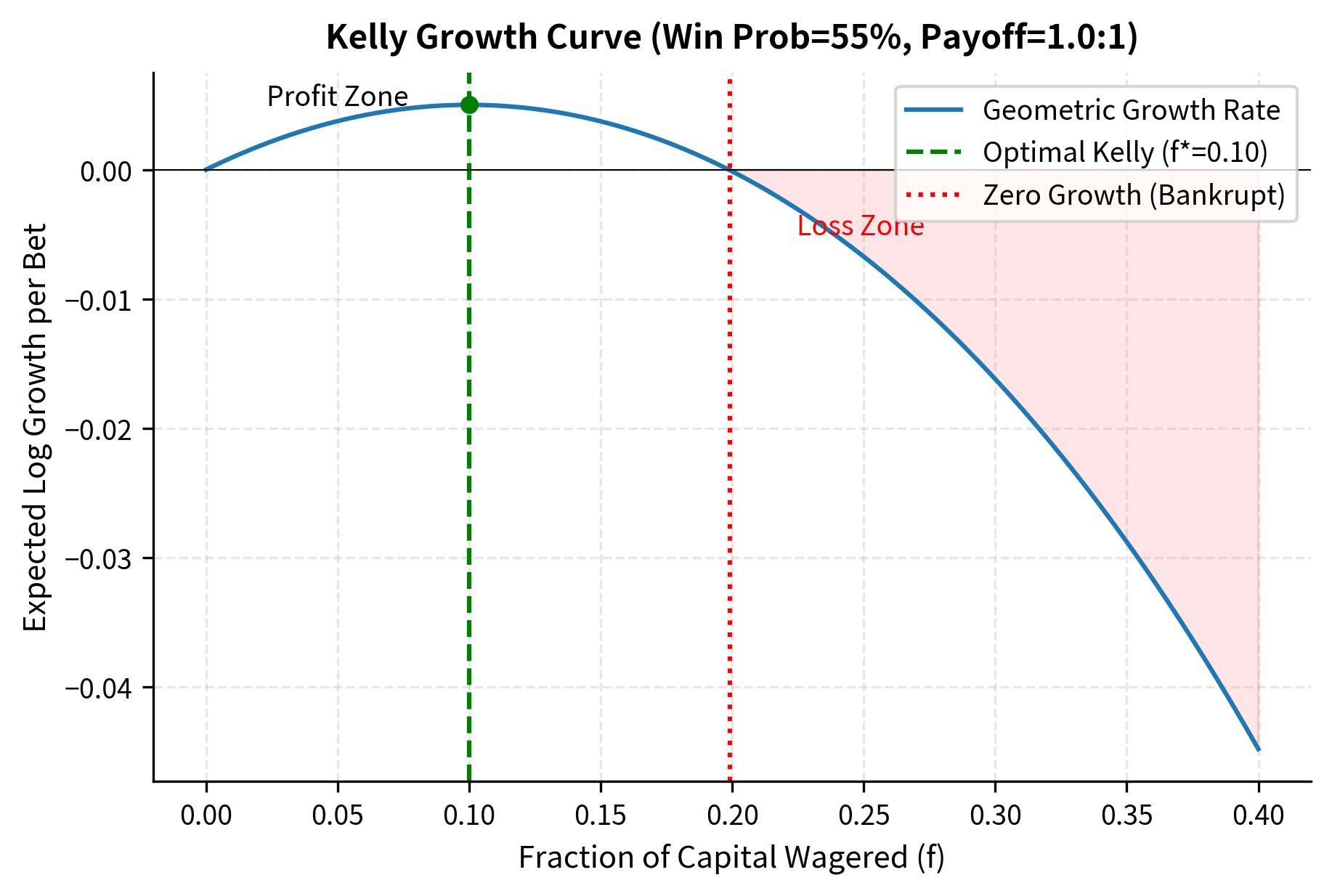
The Kelly Criterion states that to maximize the long-term geometric growth rate of capital, bet a fraction of your capital on each wager, where is the win probability, is the loss probability, and is the odds (profit per dollar wagered on a win).
Continuous Returns: Kelly for Trading
Real trading doesn't involve discrete binary outcomes. Instead, returns are continuous and approximately normally distributed over short horizons. We can derive a continuous version of the Kelly formula that applies directly to realistic trading scenarios where positions may gain or lose varying amounts.
Suppose a strategy has expected return and volatility per period. If you apply leverage (meaning you bet times your capital), your leveraged return is where . Leverage scales both the expected return and the volatility. The expected leveraged return is and the variance is . Notice that variance scales with the square of leverage, which foreshadows the extreme danger of high leverage.
For small returns, which is a reasonable approximation for daily or weekly trading, the expected log return, which determines geometric growth, is approximately:
where:
- : leveraged return
- : leverage ratio
- : expected return of the strategy
- : variance of the strategy
This approximation uses the Taylor expansion for small . The formula has a compelling structure: the first term is the expected arithmetic return, which increases linearly with leverage. The second term is the variance penalty, sometimes called "volatility drag," which increases quadratically with leverage. This quadratic penalty is why unlimited leverage is disastrous: at high enough leverage, the variance penalty overwhelms any expected return.
To maximize this geometric growth rate, we differentiate with respect to :
The derivative has two terms: represents the marginal benefit of increased leverage (more expected return), while represents the marginal cost (more variance penalty). Setting the derivative to zero identifies where these opposing forces balance:
where:
- : leverage ratio
- : expected return
- : return variance
Solving this simple equation yields the continuous Kelly leverage formula:
where:
- : optimal leverage ratio
- : expected return
- : return variance
This formula is intuitive. Optimal leverage increases with expected return, as you should bet more aggressively when the edge is larger. Optimal leverage decreases with variance, as you should bet more conservatively when uncertainty is higher. The formula can be rewritten using the Sharpe ratio :
where:
- : optimal leverage ratio
- : expected return
- : Sharpe ratio ()
- : return volatility
This alternative form reveals that optimal leverage is the Sharpe ratio divided by volatility. A strategy with higher Sharpe ratio warrants more aggressive position sizing because the edge relative to risk is larger. A strategy with lower volatility also warrants higher leverage because the same proportional bet involves less absolute risk. This formula provides the foundational insight for sizing trading positions optimally.
Properties of Kelly Betting
Kelly betting has several important mathematical properties that make it theoretically attractive:
- Maximizes geometric growth rate: No other fixed-fraction strategy achieves higher long-term wealth growth. This optimality is exact under the model assumptions.
- Never goes bankrupt: Since you only bet a fraction of capital, you always have something left, though it can become arbitrarily small. This contrasts with fixed-dollar betting, which can lead to complete ruin.
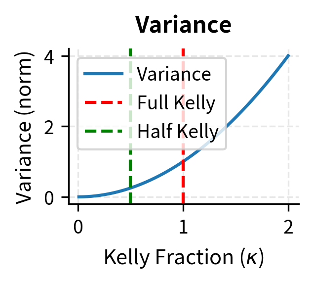
- Variance increases with leverage: At Kelly leverage, the variance of log returns equals the squared Sharpe ratio: per unit time. This provides a direct link between strategy quality and wealth volatility.
However, Kelly betting also has significant drawbacks that limit its practical applicability:
- Extreme drawdowns: Full Kelly can produce drawdowns of 50% or more with high probability, even for profitable strategies. These drawdowns are mathematically expected, not rare events, and they create severe psychological challenges for you.
- Parameter sensitivity: The optimal fraction depends critically on and , which must be estimated. Overestimating or underestimating leads to overbetting, which can be catastrophic because overbetting beyond Kelly has worse expected growth than underbetting by the same proportional amount.
- Assumes ergodicity: Kelly assumes you face the same bet repeatedly forever with unchanging parameters. Finite horizons or changing conditions violate this assumption, and the infinite-horizon optimal strategy may perform poorly over realistic investment horizons.
Fractional Kelly
Given the practical dangers of full Kelly betting, most practitioners use fractional Kelly, betting a fraction (typically 0.25 to 0.5) of the Kelly-optimal amount. This sacrifices some expected growth for substantially reduced variance and drawdown risk. The rationale is that we never know the true parameters and , so using full Kelly based on estimates is almost certainly betting too aggressively.
If we denote the Kelly fraction multiplier as , the leveraged position becomes . The multiplier represents our conservatism: is full Kelly, is half-Kelly, and is quarter-Kelly.
The expected geometric growth rate at fractional Kelly follows from substituting the scaled leverage into our growth rate formula:
where:
- : expected geometric growth rate with fractional Kelly
- : Kelly fraction multiplier ()
- : optimal full Kelly leverage
- : expected return
- : volatility
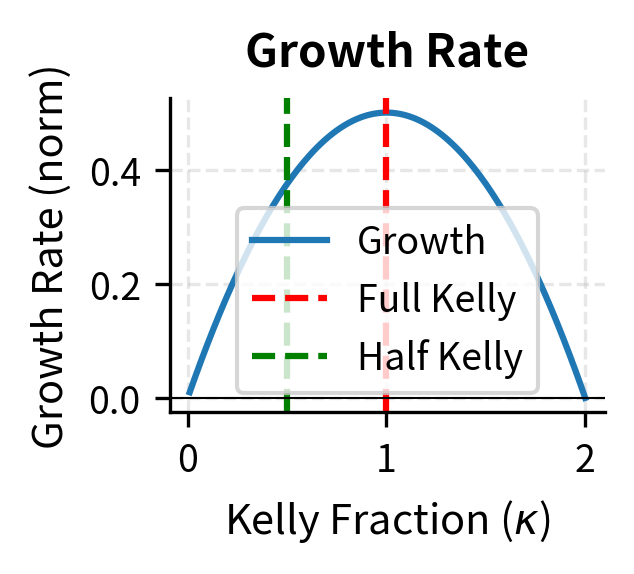
This formula reveals the fundamental tradeoff in fractional Kelly. The term in the parentheses represents growth that increases linearly with aggressiveness, while the term represents the variance penalty that increases quadratically. As increases from zero, growth initially increases faster than the penalty, but eventually the penalty dominates.
At full Kelly (), the growth rate is . At half-Kelly (), the growth rate is:
where:
- : expected geometric growth rate at half-Kelly
- : expected geometric growth rate at full Kelly
- : expected return
- : volatility
This calculation shows the efficiency of half-Kelly: it achieves 75% of the growth rate but with only 25% of the variance, since variance scales as . This tradeoff is highly attractive for risk-averse investors who value smoother wealth paths over maximum expected growth. The insight that you can sacrifice only 25% of growth while eliminating 75% of variance explains why fractional Kelly dominates practical applications.
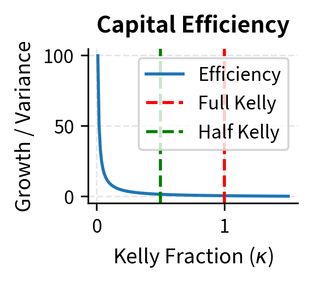
The efficiency plot reveals a crucial insight: smaller Kelly fractions provide better return per unit of risk taken. As the fraction increases toward full Kelly and beyond, efficiency deteriorates rapidly. This mathematical relationship explains why experienced practitioners almost universally advocate for conservative position sizing.
Risk Budgeting and Capital Allocation
Real portfolios contain multiple strategies, each with its own expected return, volatility, and correlations with other strategies. How should capital be allocated across strategies to maximize overall portfolio performance? This question extends Kelly's single-bet framework to the multi-dimensional setting that characterizes real trading operations.
Multi-Strategy Framework
Consider a portfolio of strategies with return vector , expected return vector , and covariance matrix . Let be the weight, or capital allocation, vector. The notation uses vectors and matrices because the interactions between strategies, captured by the covariance matrix, fundamentally affect optimal allocation.
The portfolio expected return is , which is simply the weighted average of individual strategy returns. The portfolio variance is , which accounts not only for individual strategy variances but also for all pairwise covariances. When strategies are negatively correlated, diversification reduces portfolio variance below the weighted average of individual variances.
As we discussed in Modern Portfolio Theory and Mean-Variance Optimization, the maximum Sharpe ratio portfolio solves:
where:
- : portfolio weight vector
- : expected return vector
- : covariance matrix of returns
This optimization seeks the portfolio with the best risk-adjusted return, balancing expected return in the numerator against risk in the denominator. For unconstrained optimization, which allows both leverage and short selling, the solution has a closed form:
where:
- : optimal weight vector
- : inverse covariance matrix
- : expected return vector
This is the multi-asset generalization of the Kelly criterion. Each strategy receives weight proportional to its expected return, adjusted by the inverse covariance matrix, which accounts for both individual volatility and correlations. The inverse covariance matrix effectively adjusts weights downward for volatile strategies and for strategies that are highly correlated with others, because these provide less diversification benefit.
Independent Strategies
When strategies are independent, meaning they have zero correlation with each other, the covariance matrix is diagonal: . The inverse of a diagonal matrix is simply the diagonal matrix of reciprocals. In this special case, the optimal weights simplify dramatically to:
where:
- : optimal weight for strategy
- : expected return of strategy
- : variance of strategy
This formula states that each strategy should be sized according to its individual Kelly criterion, independent of other strategies. This independence is powerful because it means you can optimize each strategy separately without worrying about interactions. The total portfolio leverage is then simply the sum of individual leverages.
For correlated strategies, the picture is more complex. Positive correlation between strategies reduces diversification benefits, and the optimal allocation accounts for this by reducing weights on highly correlated strategies. Intuitively, having two highly correlated strategies is almost like having twice the position in a single strategy, which may violate risk limits even when individual position sizes appear reasonable.
Risk Budgeting Framework
An alternative to return-based allocation is risk budgeting, where we allocate a "risk budget" to each strategy rather than capital directly. This approach is particularly useful when expected returns are uncertain but risk estimates are more reliable. In practice, volatilities and correlations tend to be more persistent and easier to estimate than expected returns, making risk budgeting a more robust framework.
The marginal risk contribution (MRC) of strategy to portfolio volatility measures how much portfolio risk increases when you slightly increase the weight of strategy . Formally, it is defined as:
where:
- : marginal risk contribution of strategy
- : portfolio volatility
- : weight of strategy
- : covariance matrix of returns
- : -th element of the marginal covariance vector
The term is the -th element of the vector obtained by multiplying the covariance matrix by the weight vector. It represents the covariance of strategy with the overall portfolio.
The total risk contribution (TRC) measures how much of the portfolio's total risk is attributable to a particular strategy. It combines the marginal contribution with the position size:
where:
- : total risk contribution of strategy
- : weight of strategy
- : marginal risk contribution
- : portfolio volatility
A fundamental property of risk contributions is that they decompose portfolio risk additively. The sum of total risk contributions equals the portfolio volatility:
where:
- : total risk contribution
- : portfolio volatility
This decomposition property means that risk contributions provide a complete accounting of where portfolio risk comes from.
In a risk budgeting framework, we specify target risk contributions (summing to 1) and find weights such that:
where:
- : total risk contribution of strategy
- : portfolio volatility
- : target risk contribution proportion for strategy
This constraint says that strategy should contribute fraction of total portfolio risk. Combining this with the definition of TRC leads to solving:
where:
- : weight of strategy
- : -th element of the vector (marginal covariance)
- : target risk budget
- : portfolio variance
This system of equations is nonlinear in the weights and typically requires numerical optimization to solve. The most common special case is equal risk contribution, where for all strategies. This equal risk contribution constraint is the foundation of risk parity approaches, which have gained substantial popularity in institutional investing.
Let's compare different allocation approaches for a three-strategy portfolio.
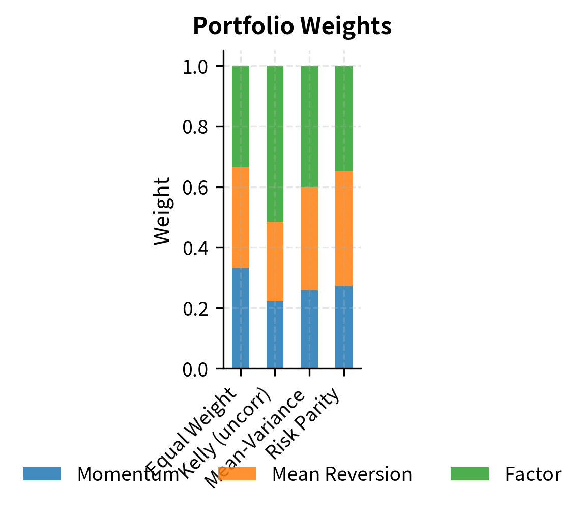
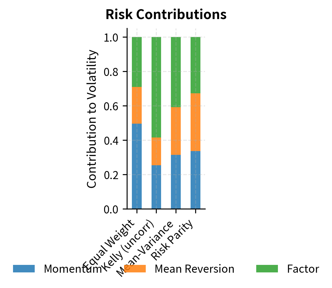
The results highlight key differences between allocation approaches:
- Equal weight treats all strategies identically regardless of their risk or return characteristics.
- Kelly/Mean-variance tilts heavily toward strategies with better risk-adjusted returns, potentially creating concentrated bets.
- Risk parity equalizes risk contribution, resulting in higher weights to lower-volatility strategies and more balanced risk exposure.
Notice that mean-variance optimization produces the highest Sharpe ratio by construction, but this comes with concentrated positions that are sensitive to estimation errors in expected returns. Risk parity sacrifices some expected return for more diversified risk exposure.
Leverage Limits and Margin Requirements
Leverage amplifies both gains and losses. While optimal sizing theory suggests an ideal leverage level, practical constraints impose hard limits on how much leverage can actually be employed. Understanding these constraints is essential for translating theoretical optimal positions into executable trades.
Understanding Margin and Leverage
When trading on margin, you borrow funds from your broker to increase position size beyond your capital. The key concepts are:
- Initial margin: The minimum equity required to open a position, typically 25-50% for stocks.
- Maintenance margin: The minimum equity required to keep a position open, typically 25-30%.
- Margin call: When equity falls below maintenance margin, requiring additional funds or position reduction.
- Leverage ratio: The ratio of total position size to equity. With 50% initial margin, maximum leverage is 2x.
For derivatives, margin works differently. Futures require "performance bond" margin representing a small percentage of notional value, enabling leverage of 10x-20x or more. Options require margin based on potential loss scenarios.
Regulation T established by the Federal Reserve, sets the initial margin requirement for most U.S. securities at 50%, implying maximum leverage of 2x. Portfolio margin accounts may receive more favorable treatment based on hedged positions and overall portfolio risk.
The Mathematics of Leverage and Drawdown
Leverage has a nonlinear relationship with drawdown risk, making high leverage more dangerous than intuition suggests. Consider a strategy with return volatility . At leverage , the leveraged volatility is . This linear scaling of volatility translates into highly nonlinear effects on drawdown probability.
Under geometric Brownian motion assumptions, the expected maximum drawdown over time horizon for a strategy with Sharpe ratio and leveraged volatility is approximately:
where:
- : expected maximum drawdown
- : leverage ratio
- : strategy volatility
- : time horizon
- : Sharpe ratio
- : inverse cumulative standard normal distribution function
The formula combines two components: a baseline volatility scaling term () and a risk-adjusted multiplier (the inverse normal term) that accounts for how the strategy's Sharpe ratio and leverage interact to determine tail risk depth. The baseline term grows with the square root of time, while the multiplier depends on the interaction between leverage and strategy quality.
A simpler approximation for the probability of experiencing a drawdown of at least follows from the reflection principle for Brownian motion:
where:
- : probability of a drawdown exceeding
- : drawdown threshold
- : leverage ratio
- : volatility
- : time horizon
This shows that drawdown probability is highly sensitive to leverage. Doubling leverage quadruples the exponent's denominator, dramatically increasing the probability of severe drawdowns. A drawdown that is virtually impossible at 1x leverage may be almost certain at 4x leverage.
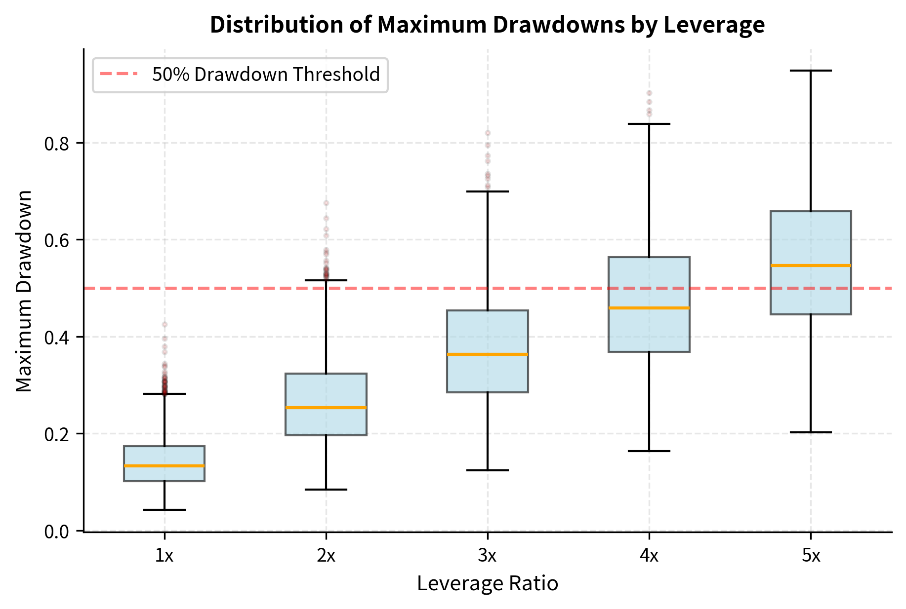
The simulation illustrates how leverage transforms a reasonable strategy into a dangerous one. At 1x leverage, this strategy with a Sharpe ratio around 0.63 has modest drawdowns. At 5x leverage, the probability of a 50%+ drawdown in a single year exceeds 50%. Recovery from a 50% drawdown requires a 100% gain, which at 10% annual returns (before the drawdown) would take nearly 7 years.
Leverage and the Risk of Ruin
Beyond drawdowns, excessive leverage creates genuine risk of ruin: losing so much capital that continuing to trade becomes impossible. Several mechanisms create this risk:
Margin calls and forced liquidation: When losses erode equity below maintenance margin, positions are forcibly closed at unfavorable prices. This "stop out" crystallizes losses that might otherwise recover.
Gap risk: Markets can move discontinuously, especially over weekends or during crises. A 3x leveraged position in an asset that gaps down 35% overnight faces a 105% loss, exceeding total capital.
Volatility expansion: Leverage is often sized based on historical volatility, but volatility can spike dramatically during crises precisely when you're already losing money.
Correlation breakdown: Strategies that appear diversified in normal conditions often become highly correlated during market stress, magnifying portfolio-level losses.
Case Studies: Leverage Disasters
History provides examples of leverage-induced failures:
Long-Term Capital Management (1998): LTCM's strategies had estimated Sharpe ratios of 1-2, but they applied leverage of 25x or more. When the Russian debt crisis triggered a flight to quality, correlations spiked and spreads widened dramatically. LTCM lost \3.6 billion bailout coordinated by the Federal Reserve to prevent systemic contagion.
Amaranth Advisors (2006): This multi-strategy fund concentrated heavily in natural gas futures. When positions moved against them, leverage of approximately 8x transformed a significant loss into a \$6 billion catastrophe wiping out the fund entirely.
XIV and Volatility ETNs (2018): Leveraged inverse volatility products lost nearly all their value in a single day during the "Volmageddon" event. A 115% spike in the VIX caused products designed to profit from calm markets to collapse.
The common thread: strategies that worked well in normal conditions failed when leverage combined with adverse market moves.
Risk Parity and Volatility Targeting
Given the dangers of leverage and the difficulties of estimating expected returns, alternative allocation frameworks focus on risk rather than return.
Risk Parity Principles
Risk parity, pioneered by Ray Dalio's Bridgewater Associates, allocates capital so that each asset contributes equally to portfolio risk. The core insight is that expected returns are notoriously difficult to estimate, but volatilities and correlations are relatively stable and predictable. By focusing on what we can estimate reliably, risk parity sidesteps much of the estimation error that plagues return-based optimization.
For a long-only portfolio where each asset contributes equally to risk (), we require:
where:
- : weight of asset
- : covariance matrix of returns
- : marginal covariance of asset
- : portfolio variance
- : number of assets
When assets are uncorrelated, this simplifies to inverse-volatility weighting:
where:
- : weight of asset
- : volatility of asset
Lower-volatility assets receive higher weights, which for traditional portfolios means bonds receive much larger allocations than stocks. To achieve competitive returns, risk parity portfolios typically apply leverage to the entire portfolio, bringing total volatility to a target level (often 10-15% annually).
Volatility Targeting
A related approach is volatility targeting, where position sizes are adjusted dynamically to maintain constant portfolio volatility. This approach recognizes that volatility varies substantially over time, so static position sizing produces varying levels of actual risk. If target volatility is and current estimated volatility is , the position multiplier is:
where:
- : leverage scaling factor at time
- : target volatility
- : estimated current volatility
This approach automatically reduces positions during high-volatility periods (when losses are most likely) and increases positions during calm periods. Research shows this can improve risk-adjusted returns and reduce drawdowns compared to constant position sizing.
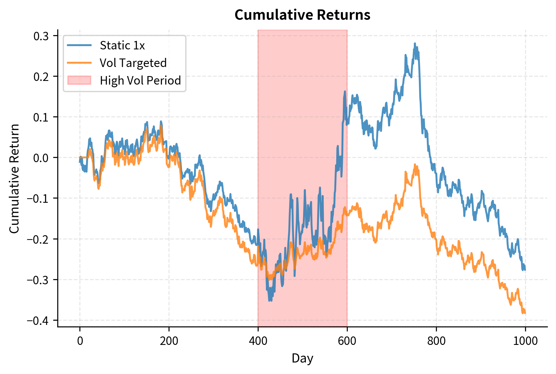
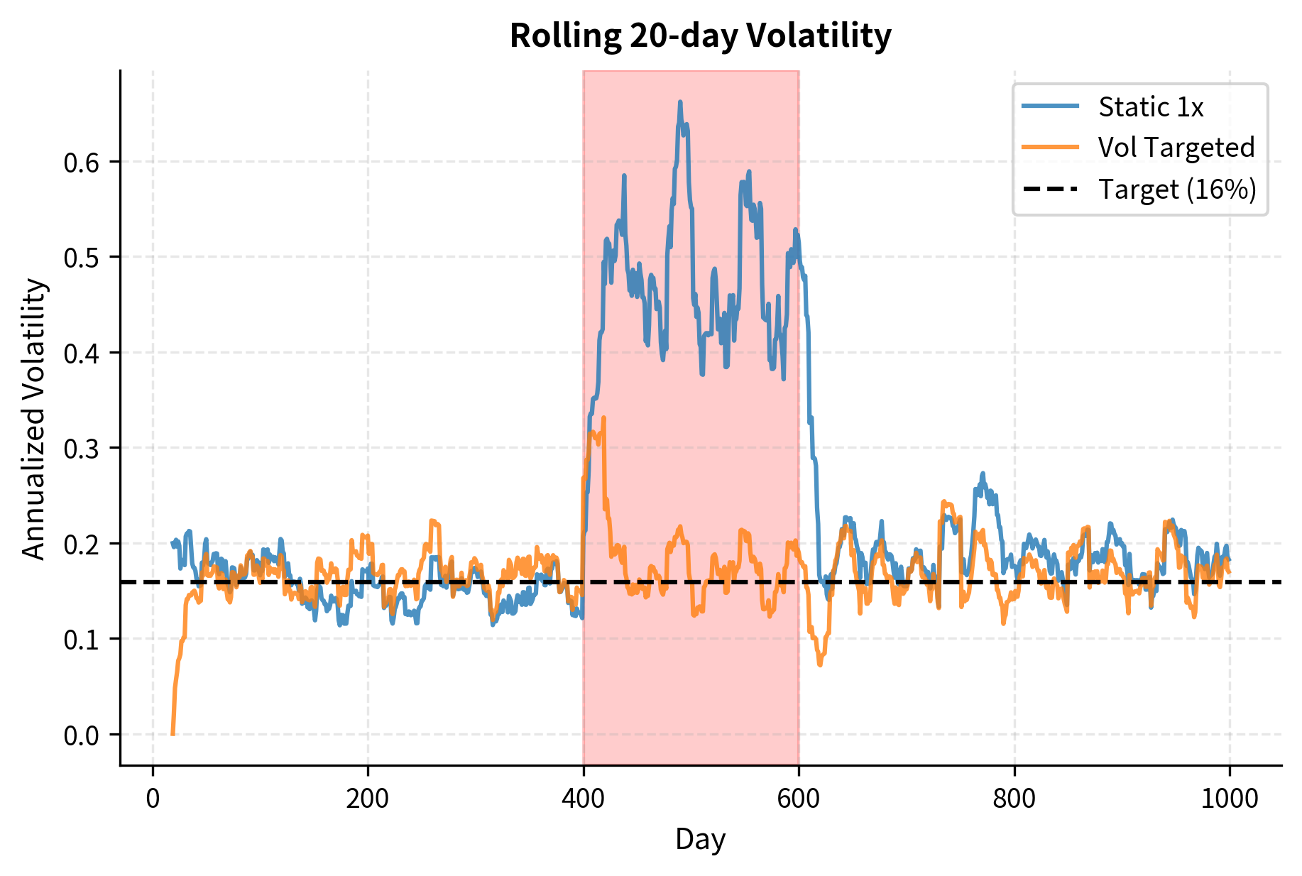
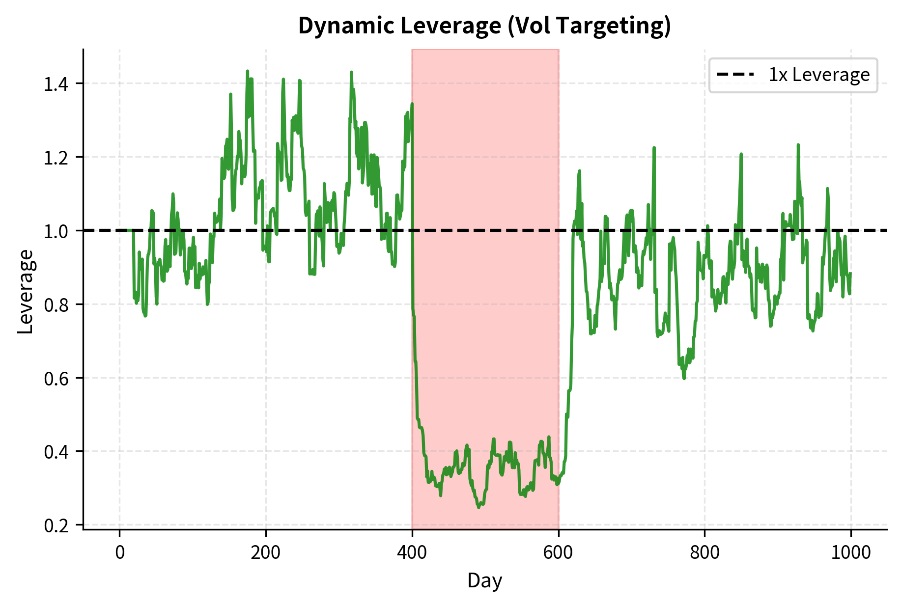
The visualization demonstrates volatility targeting's key benefit: automatic risk reduction during dangerous periods. During the simulated crisis (days 400-600), the strategy reduced leverage to well below 1x, limiting losses. After the crisis, leverage gradually increased as volatility estimates came down.
Practical Position Sizing Implementation
Let's build a comprehensive position sizing system that integrates the concepts we've covered.
Position Sizing Framework
A production position sizing system needs to handle:
- Signal to target position conversion: Translate strategy signals into desired position sizes
- Risk scaling: Apply Kelly, fractional Kelly, or volatility targeting
- Constraint enforcement: Respect leverage limits, position limits, and risk budgets
- Dynamic adjustment: Update sizes as volatility and portfolio state change
Let's test this framework with our three-strategy portfolio:
The position sizer allocates the most capital to the Factor strategy, which has the best risk-adjusted returns (Sharpe ratio 0.83). Despite Momentum having the highest expected return, its higher volatility results in a lower optimal weight. The Mean Reversion strategy's negative correlation with Momentum provides diversification benefits, earning it a meaningful allocation despite its lower expected return.
Drawdown-Based Position Adjustment
Many practitioners reduce position sizes following drawdowns, either as a risk management discipline or to preserve capital for potential mean reversion opportunities. This can be formalized:
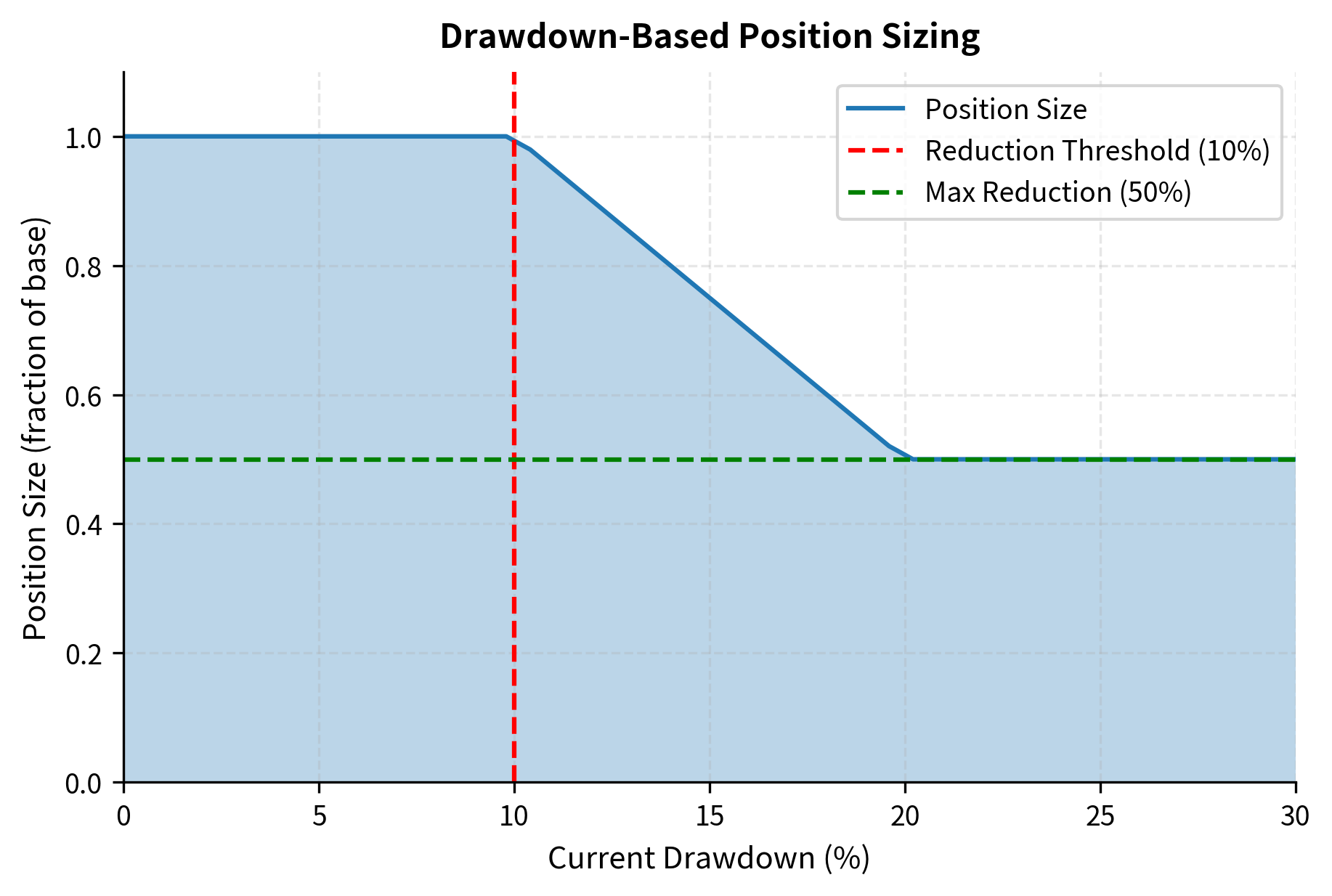
This drawdown-based adjustment provides automatic de-risking during losing periods. While it may reduce returns during recoveries, it helps preserve capital and reduces the psychological burden of maintaining full positions during painful drawdowns.
Limitations and Practical Considerations
Position sizing theory provides valuable guidance, but several limitations affect real-world implementation.
Parameter estimation uncertainty: The Kelly formula requires accurate estimates of expected return and volatility. In practice, expected returns are notoriously difficult to estimate. An overestimate of by 50% leads to a 50% overestimate of optimal leverage, potentially disastrous during adverse conditions. This uncertainty is the primary reason practitioners use fractional Kelly, treating the formula's output as an upper bound rather than a target.
Non-stationarity: Financial return distributions change over time. Volatility clusters, correlations spike during crises, and regime changes alter expected returns. Position sizing calibrated to historical parameters may be dramatically wrong for future conditions. Dynamic approaches like volatility targeting partially address this by continuously re-estimating parameters.
Model misspecification: The continuous Kelly derivation assumes normally distributed returns. Real returns exhibit fat tails, meaning extreme events occur far more frequently than Gaussian models predict. A "5-sigma" event that should occur once in 7,000 years under normality happens roughly once per decade in markets. Tail risk makes any fixed-fraction betting strategy vulnerable to catastrophic losses during extreme events.
Liquidity and market impact: As discussed in Transaction Costs and Market Impact, large positions affect prices. The theoretical optimal position may not be achievable without significant market impact, and forced liquidation during drawdowns occurs at the worst possible prices. Position sizing must account for realistic execution constraints, particularly for strategies operating in less liquid markets.
Correlation instability: Diversification benefits assumed when allocating across strategies depend on correlation estimates. During market crises, correlations typically spike toward 1.0, exactly when diversification is most needed. Portfolio-level position sizing should stress-test performance under elevated correlation scenarios.
Despite these limitations, the frameworks presented remain valuable for several reasons. First, they provide quantitative discipline, replacing intuition-based sizing with principled analysis. Second, they clarify the tradeoffs between growth and risk, helping you choose appropriate points on the risk spectrum. Third, they highlight the extreme sensitivity of outcomes to leverage, encouraging conservative approaches. Even imperfect Kelly estimates, scaled down by fractional multipliers and capped by leverage constraints, produce more robust position sizing than ad hoc approaches.
Summary
Position sizing determines whether a trading edge compounds into wealth or destruction. This chapter developed the mathematical foundations and practical frameworks for optimal sizing:
Kelly Criterion fundamentals: The Kelly formula maximizes long-term geometric growth by betting a fraction in the discrete case or applying leverage in the continuous case. Full Kelly betting is aggressive, often too aggressive for practical use.
Fractional Kelly: Using 25-50% of Kelly-optimal sizing sacrifices modest growth for substantially reduced variance and drawdown risk. Half-Kelly achieves 75% of Kelly growth with 25% of the variance, an attractive tradeoff for most investors.
Multi-strategy allocation: For portfolios of strategies, optimal allocation follows , generalizing Kelly to account for correlations. Strategies with better risk-adjusted returns and lower correlation receive higher weights.
Risk budgeting: When expected returns are uncertain, risk parity approaches allocate based on risk contribution rather than expected return. This produces more robust portfolios, though potentially at the cost of expected return.
Leverage dangers: Leverage amplifies both gains and losses nonlinearly. Maximum drawdown probability increases dramatically with leverage, and numerous historical examples demonstrate how excessive leverage has destroyed sophisticated investors. Practical constraints on gross leverage, position limits, and margin requirements provide essential guardrails.
Volatility targeting: Dynamic position sizing based on current volatility estimates automatically reduces risk during dangerous periods. This approach has demonstrated ability to improve risk-adjusted returns across many asset classes and strategies.
The next chapter addresses ethical and regulatory considerations in quantitative trading, examining how position sizing and trading practices intersect with market integrity and investor protection requirements.
Quiz
Ready to test your understanding? Take this quick quiz to reinforce what you've learned about position sizing, the Kelly Criterion, and leverage management.

Comments