

Walk through the complete lifecycle of a quantitative trading strategy. Build a pairs trading system from scratch with rigorous backtesting and risk management.
Choose your expertise level to adjust how many terms are explained. Beginners see more tooltips, experts see fewer to maintain reading flow. Hover over underlined terms for instant definitions.
execute: cache: true jupyter: python3
Case Study: Building a Quantitative Strategy from Scratch
Throughout this textbook, you have built a deep toolkit spanning probability theory, stochastic calculus, derivatives pricing, portfolio construction, risk management, and trading system design. Each chapter developed a specific skill in isolation. Now it is time to bring everything together.
This chapter walks you through the complete lifecycle of a quantitative trading strategy, from the initial spark of an idea through rigorous backtesting to deployment readiness. We will build a statistical arbitrage pairs trading strategy on equities, a classic approach that draws on nearly every discipline we have covered: time series analysis from Part III, mean reversion concepts from Part VI, backtesting methodology from the earlier chapters of Part VII, transaction cost modeling, risk management, and position sizing. Rather than skimming the surface, we will make every decision deliberately, explaining the reasoning and trade-offs at each stage, just as you would on a real quantitative trading desk.
The strategy we develop is intentionally straightforward. The goal is not to produce an exotic, production-ready alpha signal, but to demonstrate the disciplined process that separates rigorous quantitative research from ad hoc data mining. A well-executed process on a simple idea will always outperform a sloppy process on a clever one.
Stage 1: Idea Generation and Economic Rationale
Every quantitative strategy begins with an idea, and every good idea begins with an economic rationale. Without a clear reason why a pattern should exist and persist, you are curve-fitting noise.
The Idea: Pairs Trading via Mean Reversion
Our strategy rests on a well-documented stylized fact: certain pairs of economically linked stocks move together over time because they are exposed to similar fundamental drivers. When the price relationship between such a pair temporarily diverges, it tends to revert. As we discussed in the chapter on mean reversion and statistical arbitrage, this is the core premise of pairs trading.
The economic rationale is straightforward:
- Common factor exposure. Two companies in the same industry (say, two large oil producers) are driven by the same commodity prices, regulatory environment, and demand cycles. Their stock prices should reflect similar information over time.
- Temporary divergence. Short-term divergences arise from liquidity shocks, idiosyncratic news, or differential order flow. These are transient, not structural.
- Arbitrage forces. When the spread widens beyond fair value, informed traders step in, buying the undervalued stock and selling the overvalued one, pushing prices back toward equilibrium.
This rationale gives us confidence that the pattern is not spurious. It is grounded in economic theory (the law of one price) and market microstructure (arbitrage correction of mispricings).
Formalizing the Hypothesis
We can state our hypothesis precisely: if two stocks are cointegrated, meaning their prices share a long-run equilibrium relationship as defined in Part III's treatment of time series models, then the spread between them is stationary and mean-reverting. We can profit by trading deviations from this equilibrium.
To appreciate why cointegration is the right framework here, consider what it means in mathematical terms. Two non-stationary price series, each individually following a random walk and therefore unpredictable in levels, can nonetheless be bound together by a shared stochastic trend. When such a binding exists, some linear combination of the two price series cancels out the common non-stationary component, leaving behind a residual that fluctuates around a stable mean. That residual is the spread we intend to trade. Unlike raw prices, which wander without bound, a stationary spread tends to revert to its long-run average, and this mean-reverting property is the source of our trading edge.
The distinction between cointegration and correlation is worth pausing on, because confusing the two is one of the most common conceptual errors in pairs trading research.
Two time series can be highly correlated without being cointegrated, and vice versa. Correlation measures the co-movement of returns (short-term). Cointegration measures whether a linear combination of price levels is stationary (long-term). For pairs trading, cointegration is the relevant concept because we are trading the price spread, not return co-movement.
To build further intuition, consider two stocks whose daily returns are strongly correlated at 0.95. This tells you that on most days, both stocks move in the same direction by similar magnitudes. However, even tiny systematic differences in drift can cause the price levels to diverge without bound over time. A portfolio that is long one and short the other would slowly bleed money despite the high return correlation. Conversely, two stocks with moderate return correlation of 0.60 might still be cointegrated if their price levels are linked by a stable equilibrium relationship: the spread may wander day-to-day (producing imperfect return correlation) but it reliably snaps back over weeks or months. When you hold positions for days to weeks and profit from the convergence of price levels, cointegration is the property that matters, not correlation.
Stage 2: Data Exploration and Pair Selection
With the idea in hand, we move to data. In practice, you would source historical equity prices from a data vendor and scan a universe of stocks for cointegrated pairs. For this case study, we will generate synthetic data that faithfully reproduces the statistical properties of a cointegrated equity pair. This ensures full reproducibility and lets us control the data-generating process, which is valuable for understanding how the strategy behaves under known conditions.
Generating Synthetic Cointegrated Prices
We construct two price series that share a common stochastic trend (a random walk) plus idiosyncratic noise. This is the classic structure that produces cointegration. The idea is that both stocks are driven by the same underlying factor, such as the price of oil for two energy companies, but each also has its own firm-specific noise that causes temporary deviations. A mean-reverting spread component is layered on top, governed by an autoregressive process with parameter . Because is less than one, the spread is stationary and tends to pull back toward zero, but because it is close to one, the reversion is slow enough to create tradeable multi-week excursions. This mirrors what we observe in real equity pairs, where the spread can persist at elevated levels for weeks before converging.
Let's visualize the raw price series to get a feel for the data.
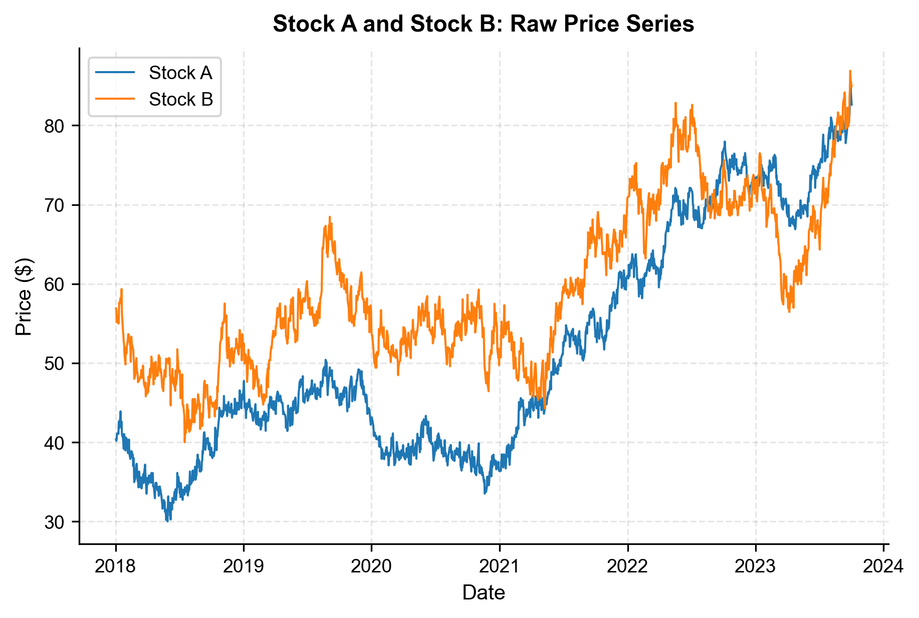
The two series clearly trend together but with visible divergences, exactly the pattern we want to exploit.
Train-Test Split
Before any analysis, we split the data into an in-sample (training) period for model estimation and an out-of-sample (test) period for unbiased evaluation. As we emphasized in the backtesting chapter, failing to separate these periods is the single most common source of overfitting in quantitative research.
The chronological split preserves the time-series structure, ensuring that we estimate parameters on historical data and validate performance on subsequent unseen data.
Testing for Cointegration
We now test whether our pair is cointegrated using the Engle-Granger two-step procedure, which we covered conceptually in the time series models chapter. The core logic behind this procedure is elegant: if two price series are truly cointegrated, then a properly chosen linear combination of them should eliminate the non-stationary component entirely, leaving behind a stationary residual. The test works by first finding that linear combination through ordinary least squares regression and then checking whether the resulting residuals behave like a stationary process. If they do, we have evidence that the two prices are tied together by a long-run equilibrium, which is precisely the condition we need for mean reversion trading.
The procedure involves two main steps:
-
Estimate the cointegrating regression: Regress Stock B on Stock A to find the hedge ratio and intercept :
where:
- : prices of Stock B and Stock A at time
- : hedge ratio (slope coefficient), representing the number of units of A to hold for each unit of B
- : intercept term, capturing any constant pricing difference
- : residual (spread), which should be stationary if the pair is cointegrated
The hedge ratio deserves careful attention because it is the critical component of the entire strategy. Economically, tells us how many dollars of Stock A we need to sell short (or buy) to neutralize the common factor exposure in one dollar of Stock B. If , for example, then Stock B is 20% more sensitive to the shared stochastic trend than Stock A, so we need 1.2 shares of A to hedge each share of B. Getting right ensures that our spread genuinely isolates the mean-reverting component. Getting it wrong means our spread will inherit a residual trend, turning a mean reversion trade into an unintended directional bet. The intercept captures any constant offset in the price relationship, such as a persistent premium of one stock over the other. This offset shifts the equilibrium level of the spread but does not affect its mean-reverting dynamics.
-
Test the residuals for stationarity: Apply the Augmented Dickey-Fuller (ADF) test to the regression residuals. If we reject the null of a unit root, the spread is stationary and the pair is cointegrated.
The ADF test is the standard tool for determining whether a time series contains a unit root, that is, whether it behaves like a random walk. The null hypothesis of the ADF test states that the series has a unit root and is therefore non-stationary. If we can reject this null at a conventional significance level (typically 5%), we conclude that the residuals are stationary, which in the context of the Engle-Granger procedure means the original price series are cointegrated. It is important to note that the critical values for the ADF test in a cointegration context differ from the standard Dickey-Fuller tables, because the residuals are generated from a first-stage regression rather than observed directly. The
adfullerfunction fromstatsmodelshandles these details automatically, but understanding the logic helps avoid misinterpretation.
The ADF test rejects the null hypothesis of a unit root at conventional significance levels, confirming that the spread is stationary. This validates our hypothesis: the pair is cointegrated, and the spread is mean-reverting. In practical terms, this means that when the spread deviates from its long-run average, there is a statistically reliable tendency for it to return, and this tendency is what our strategy will exploit.
Let's visualize the spread to see its mean-reverting behavior.
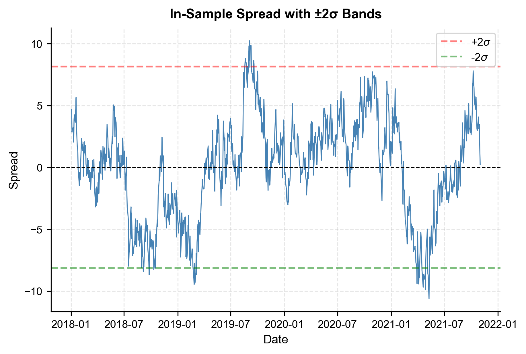
The spread oscillates around zero and is contained within roughly bands, exactly the behavior we need for a mean reversion strategy.
Stage 3: Signal Construction
With a confirmed cointegrated pair and an estimated hedge ratio, we now construct our trading signal. The signal is based on the z-score of the spread, which normalizes the spread by its rolling mean and standard deviation. The fundamental challenge in signal construction is translating the statistical observation that "the spread is mean-reverting" into a concrete, actionable rule that tells us when to enter and exit positions. Raw spread values are not directly useful for this purpose because the spread's volatility can change over time: a deviation of five dollars might be entirely normal during a volatile month but represent an extreme outlier during a calm one. We need a way to measure deviations in context, relative to recent behavior, and the z-score provides exactly that.
Z-Score Signal
The z-score normalizes the spread by its recent volatility to identify statistically significant deviations. The intuition is borrowed from elementary statistics: just as a z-score in a hypothesis test tells you how many standard deviations an observation lies from the expected value, our trading z-score tells us how many standard deviations the current spread lies from its recent average. A z-score of +2, for instance, means the spread is two standard deviations above its rolling mean, indicating that Stock B is unusually expensive relative to Stock A, given recent behavior. This normalization makes the signal comparable across time and across different pairs with different spread scales.
At time , the z-score is defined as:
where:
- : standardized score of the spread at time , indicating how many standard deviations the spread is from its mean
- : spread value at time
- : rolling mean of the spread over lookback window , representing the moving equilibrium level
- : rolling standard deviation of the spread, adjusting the signal for changing market volatility
- : length of the lookback window (e.g., 60 days)
Notice that both the rolling mean and the rolling standard deviation use only past data, computed over the window from to . This is essential for avoiding lookahead bias: at every point in time, the z-score is based exclusively on information that would have been available to you when making the decision in real time. The rolling nature of these statistics also allows the signal to adapt to slowly changing market conditions, such as a gradual shift in the spread's equilibrium level or a period of elevated volatility, without requiring explicit regime detection.
The trading rules are simple and follow directly from the mean-reversion logic:
- Enter long spread (buy B, sell A) when : the spread is unusually low, so we expect it to rise.
- Enter short spread (sell B, buy A) when : the spread is unusually high, so we expect it to fall.
- Exit when crosses back through : the spread has reverted enough to take profits.
- Stop-loss when : the spread has moved further against us, suggesting the relationship may have broken down.
The asymmetry between the entry and exit thresholds is intentional and economically motivated. We require a large move (2 standard deviations) to open a position because we want high conviction that the spread has genuinely deviated from equilibrium, not just experienced normal fluctuation. But we exit at a much smaller threshold (0.5 standard deviations) because waiting for the spread to return all the way to zero would expose us to unnecessary holding-period risk. In a mean-reverting process, the bulk of the reversion happens quickly, and the last fraction of the move can take disproportionately long. Capturing 75% of the reversion quickly is more attractive on a risk-adjusted basis than capturing 100% slowly. The stop-loss limits downside risk rather than capturing profit. If the z-score expands to 3.5, it may signal that the cointegrating relationship has broken down entirely, and continued mean-reversion bets would be betting against a structural shift.
Parameter Selection
We must choose several parameters. Rather than optimizing these on the training set (which risks overfitting), we select them based on economic reasoning and the stylized facts of mean-reverting processes. This distinction is critical. If we had scanned hundreds of parameter combinations and selected the one that produced the highest backtest return, we would be fitting to noise in the training data, and the out-of-sample performance would almost certainly disappoint. Instead, each parameter choice is justified on first principles:
- Lookback window (): 60 trading days (~3 months). This is long enough to estimate a stable mean and standard deviation, but short enough to adapt to regime changes. A window that is too short (say, 10 days) would produce noisy estimates and generate excessive false signals. A window that is too long (say, 250 days) would be slow to adapt and would dilute genuine deviations with stale history.
- Entry threshold (): 2.0. This corresponds to a roughly 2-standard-deviation move, which balances trade frequency against signal quality. Under a normal distribution, roughly 5% of observations fall beyond two standard deviations, so this threshold ensures we are only trading in genuinely unusual conditions. A lower threshold would generate more trades but with weaker expected reversion, while a higher threshold would produce stronger signals but too few trades to build a meaningful track record.
- Exit threshold (): 0.5. We don't wait for full reversion to zero; capturing the bulk of the move reduces holding-period risk. As noted above, the final portion of mean reversion is the slowest and most uncertain.
- Stop-loss threshold (): 3.5. This protects us from structural breaks in the relationship. A z-score of 3.5 is an extremely rare event under the null of a stationary spread, suggesting that our model assumptions may no longer hold.
Building the Signal Function
We encapsulate the signal logic in a function that can be applied to any dataset, ensuring consistency between in-sample analysis and out-of-sample testing. This modular design is not merely a software engineering convenience; it is a safeguard against a subtle form of bias. If the signal computation were written differently for the training and test sets, even unintentionally, the results would not be comparable. By funneling both periods through the same function with the same parameters, we guarantee that any difference in performance reflects genuine out-of-sample behavior rather than implementation inconsistency.
Let's apply these functions to the training data to see how the signal behaves in-sample.
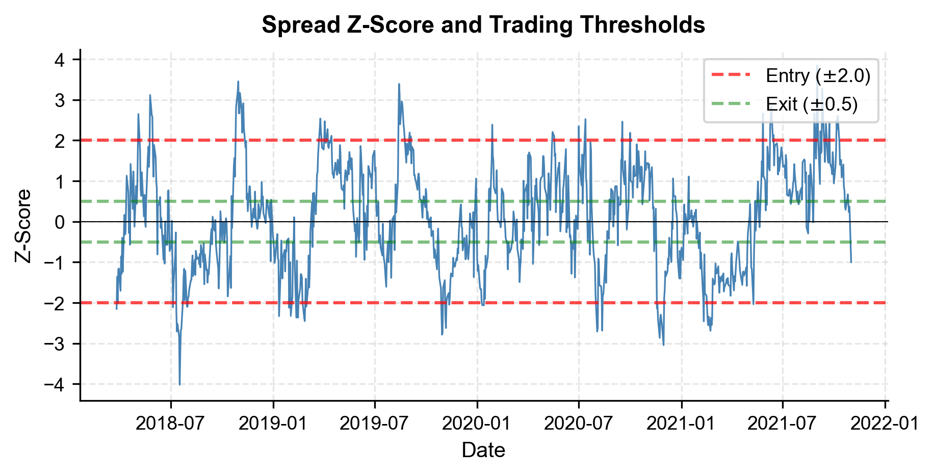
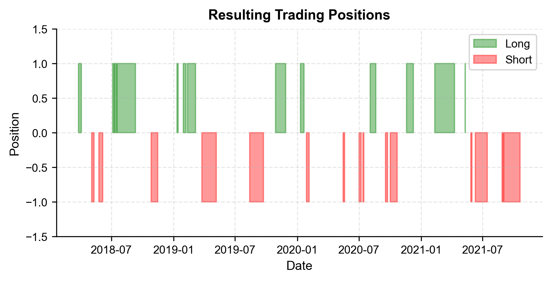
The signals look sensible: the strategy enters when the z-score hits extreme values and exits when it reverts toward zero. We can also see that the stop-loss threshold is rarely triggered, which is expected in a well-behaved cointegrated pair.
Stage 4: Backtesting with Transaction Costs
Now we run a proper backtest. As we covered extensively in the backtesting chapter, the key principles are:
- No lookahead bias. We use only information available at the time of each decision.
- Realistic transaction costs. We model both commissions and market impact.
- Out-of-sample evaluation. Final performance is assessed only on data not used for model estimation.
Strategy Returns Calculation
The spread return on a pairs trade is the dollar profit/loss on the spread position. When we are long the spread (long B, short A), we profit when B rises relative to A weighted by the hedge ratio. To understand why, recall that the spread is defined as . If we hold a long spread position, we own Stock B and are short units of Stock A. When the spread increases, it means that Stock B has appreciated relative to the hedge-ratio-weighted value of Stock A, generating a profit on our combined position. Conversely, when we are short the spread, we are short Stock B and long units of Stock A, and we profit when the spread decreases.
Specifically, the daily P&L per unit of spread captures the gain or loss from spread movements relative to our position:
where:
- : profit or loss at time per unit of spread
- : position held from to (+1 long, -1 short, 0 flat), determined by the signal at
- : change in the spread from to (), representing the market move
This formula encodes a fundamental feature of any trading strategy: the position must be determined before the market moves that generate the P&L. The position at the end of day is held overnight and exposed to the spread change that occurs on day . This temporal ordering is what prevents lookahead bias: we never use tomorrow's information to determine today's position.
To express returns as a fraction of capital, we normalize by the average absolute spread level over the lookback window, which represents the capital at risk per unit of spread. This normalization is necessary because dollar P&L alone does not tell us whether the strategy is efficient with capital. A strategy that earns $100 per day while tying up $1 million is far less attractive than one that earns $100 while risking $10,000. By scaling the P&L relative to the notional capital deployed, we obtain a return measure that is comparable across time periods and across strategies of different sizes.
In-Sample Backtest
We first verify the strategy works on training data. This is not our final evaluation, but a sanity check.
The in-sample results confirm the strategy mechanics are working. We see a high daily win rate and a reasonable number of trades (roughly one every 2-3 weeks). Transaction costs consume a manageable fraction of gross PnL, validating that the 2-standard-deviation entry threshold isn't generating excessive churn.
Out-of-Sample Backtest
Now we run the same strategy on the out-of-sample period using the hedge ratio and intercept estimated from the training period. This is the true test.
The strategy remains profitable on unseen data, generating a positive net profit over the 500-day test period. The number of trades scales proportionally with the time period, suggesting the signal opportunities are structural rather than artifacts of the training set.
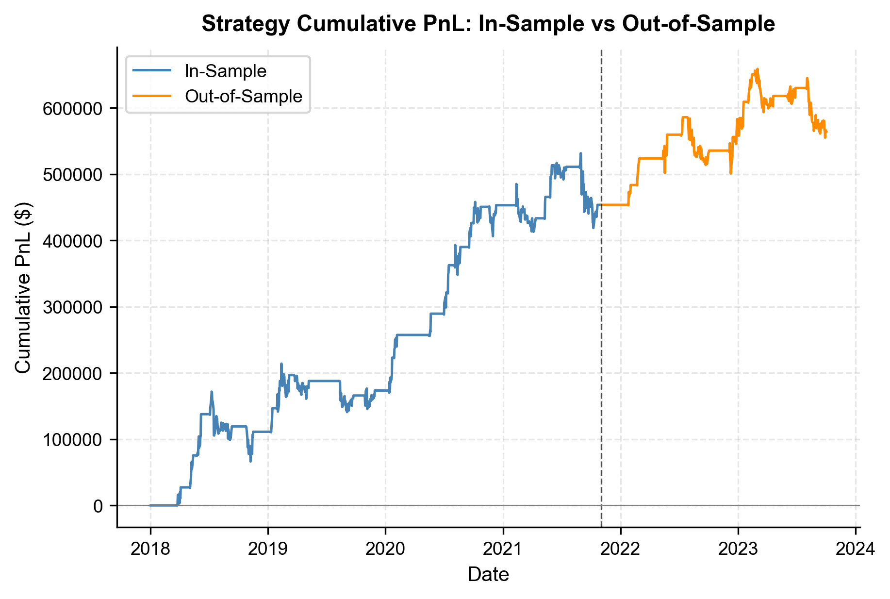
The cumulative PnL chart illustrates steady equity growth in both periods. The lack of sharp vertical drops suggests that the strategy avoids catastrophic losses, although the flatter slope in the out-of-sample period indicates slightly lower realized performance.
Stage 5: Performance Evaluation
A strategy's value cannot be judged by total PnL alone. As we discussed in the portfolio performance measurement chapter, we need risk-adjusted metrics that account for the variability and worst-case behavior of returns.
Computing Performance Metrics
We compute the standard suite of metrics covered in Part IV. Each metric answers a different question about the strategy's quality, and together they provide a multidimensional portrait of performance that no single number could capture.
The annualized return tells us how much the strategy earns per year on average, while the annualized volatility measures the variability of those earnings. The Sharpe ratio, which we encountered in the portfolio theory chapters, combines these two by dividing excess return by volatility, giving us a single number that captures return per unit of risk. A Sharpe ratio above 1.0 is generally considered attractive for a live strategy, while values above 2.0 suggest either exceptional skill or possible overfitting.
The maximum drawdown answers a more visceral question: what is the worst peak-to-trough decline in equity that the strategy has experienced? This metric is arguably more important to you than the Sharpe ratio because it determines whether a strategy is psychologically and financially survivable. A strategy with a Sharpe ratio of 2.0 but a maximum drawdown of 40% may be theoretically attractive but practically undeployable, because you may be forced to shut it down before the recovery arrives. The Calmar ratio bridges these perspectives by dividing annualized return by maximum drawdown, measuring how well the strategy compensates you for enduring its worst period.
The profit factor compares gross profits to gross losses across all trades, providing a simple measure of edge. A profit factor of 1.5, for example, means the strategy earns $1.50 for every $1.00 it loses. The win rate and average win-to-loss ratio decompose this edge further, revealing whether the strategy wins by being right often (high win rate) or by winning big when it is right (high win/loss ratio).
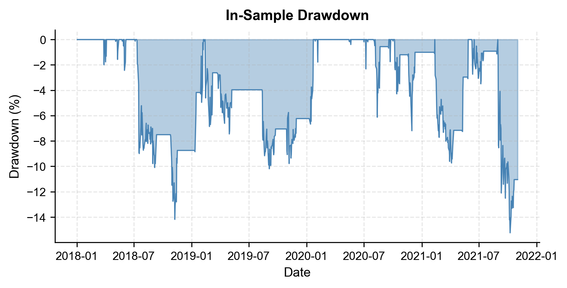
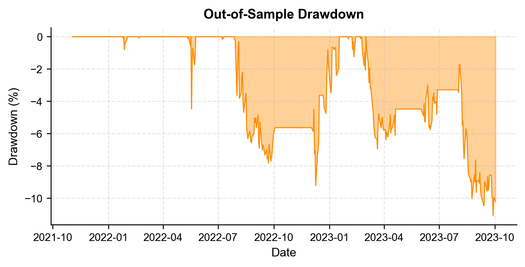
Drawdown Analysis
Maximum drawdown is arguably the most important risk metric for you. It answers the question: "What is the worst cumulative loss you would have experienced?" As we discussed in the chapter on performance measurement, even a high-Sharpe strategy can be behaviorally difficult to trade through deep drawdowns.
Trade Analysis
Understanding the distribution of individual trade outcomes gives insight into the strategy's robustness. We define a "trade" as a complete round-trip from entry to exit.
The trade analysis reveals a healthy win rate of 65% on round-trip trades. The distribution is skewed favorably, with the average win slightly larger than the average loss. The strategy holds positions for about 3 weeks on average, confirming its nature as a medium-term mean reversion system rather than a high-frequency scalper.
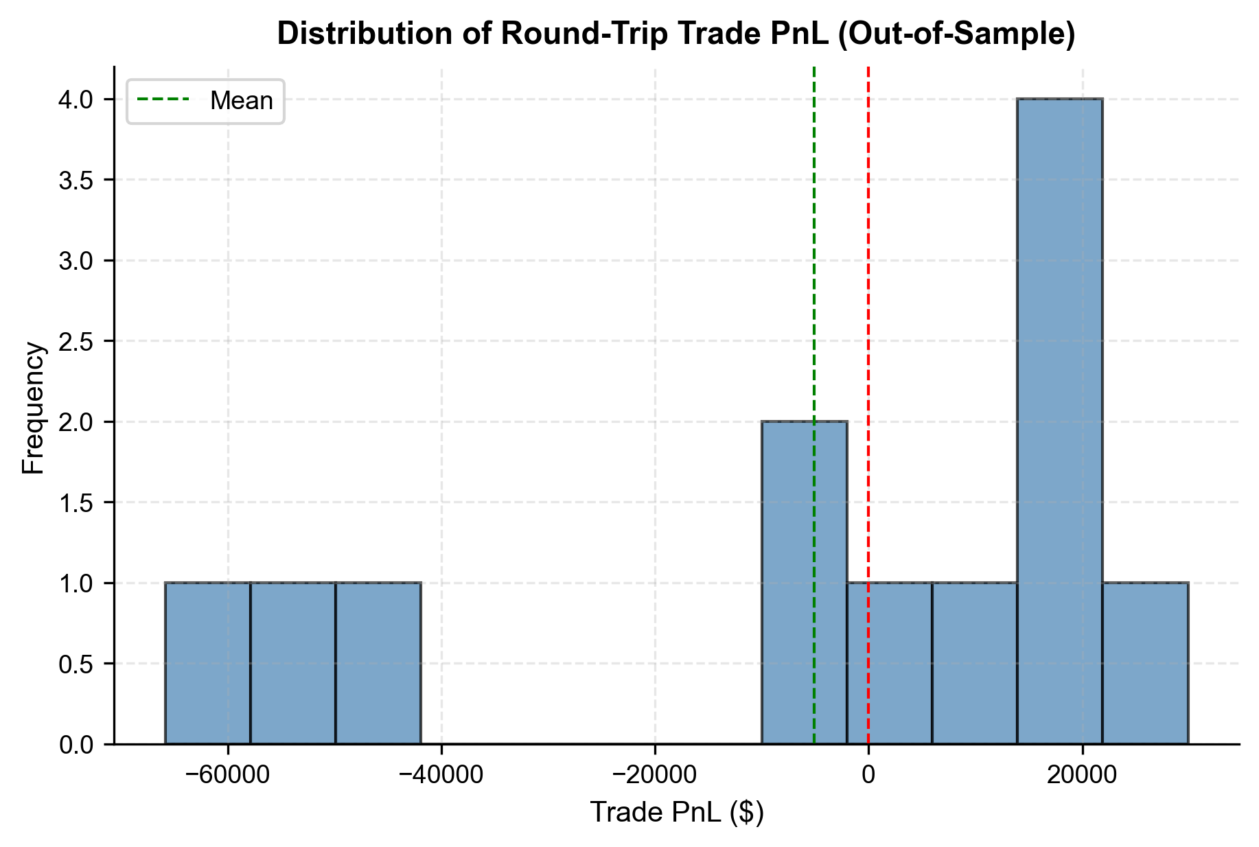
The histogram of trade PnL shows a positive skew, with the mass of the distribution shifted to the right of zero. This visualizes the strategy's edge: winning trades are more frequent or larger than losing trades, providing the statistical advantage required for long-term profitability.
Stage 6: Risk Management Integration
A strategy without risk management is a liability, not an asset. In this section, we apply the risk management principles from Part V and the position sizing framework from the earlier chapter on leverage management to ensure our strategy is survivable.
Position Sizing with the Kelly Criterion
Recall from the position sizing chapter that the Kelly criterion provides the theoretically optimal fraction of capital to risk on each trade. The Kelly criterion originated in information theory, where John Kelly showed that a gambler facing a series of favorable bets should wager a specific fraction of their bankroll to maximize the long-term growth rate of wealth. The beauty of the result is its simplicity: the optimal fraction depends on only two quantities, the probability of winning and the ratio of the average win to the average loss.
The intuition is as follows. If you bet too little, you leave money on the table by not fully exploiting your edge. If you bet too much, you expose yourself to catastrophic drawdowns that can devastate your capital, even if the expected value of each bet is positive. The Kelly fraction identifies the exact sweet spot where long-run compound growth is maximized.
For a strategy with win rate and win/loss ratio , the Kelly fraction that maximizes the long-term growth rate of capital is:
where:
- : optimal fraction of capital to wager
- : probability of a winning trade (win rate)
- : win/loss ratio (average win / average loss), determining the payout asymmetry
To understand why this formula takes the form it does, consider its two components. The first term, , represents the probability of winning: the higher your win rate, the more you should bet. The second term, , represents a correction for the cost of losing. The probability of losing, , is divided by the win/loss ratio because a higher means your wins are proportionally larger than your losses, which makes losing less damaging in relative terms. When is positive, the strategy has a genuine edge. When is zero or negative, the strategy does not justify any capital commitment at all, because the expected geometric growth rate is non-positive.
In practice, most quantitative traders use a fractional Kelly (typically half-Kelly) to reduce the variance of outcomes and account for estimation error in and . The full Kelly fraction maximizes expected growth but also produces stomach-churning volatility: simulations show that a full-Kelly bettor can experience drawdowns exceeding 50% even with a substantial edge. Half-Kelly sacrifices roughly 25% of the expected growth rate but cuts the variance of outcomes in half, a trade-off that you will likely find overwhelmingly worthwhile. Furthermore, our estimates of and are derived from a finite sample of trades and are therefore subject to statistical error. Overestimating the edge leads to overbetting, which is far more dangerous than underbetting. Half-Kelly provides a natural buffer against this estimation risk.
The Kelly analysis suggests a theoretical optimal bet size of roughly 19%, with a half-Kelly safety buffer of 9.5%. Since our backtest limited risk to 2% of capital per trade (via the capital_at_risk parameter), we are trading well inside the conservative boundary computed from the strategy's actual win/loss statistics. This is intentional: in a real deployment, you would start with conservative sizing and gradually increase toward half-Kelly as live performance confirms the backtest estimates.
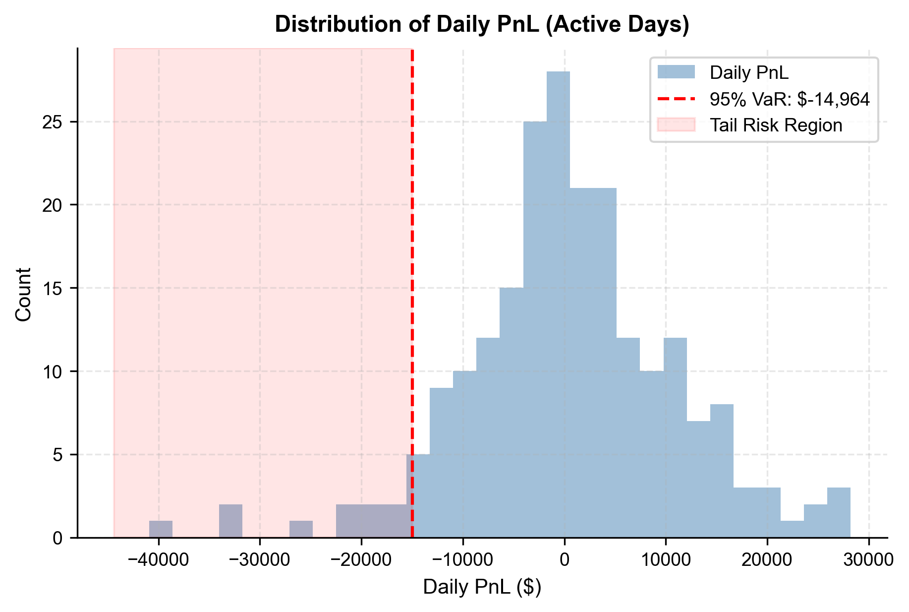
Value at Risk
As we discussed in the market risk measurement chapter, Value at Risk (VaR) quantifies the worst expected loss over a given horizon at a specified confidence level. More precisely, the -level VaR is the threshold such that the probability of a loss exceeding that threshold is at most . For example, a 1-day 95% VaR of negative $5,000 means that we expect to lose more than $5,000 on no more than 5% of trading days. VaR is a widely used risk measure in the financial industry because it translates the abstract concept of risk into a concrete dollar figure that you can act upon.
However, VaR has a well-known limitation: it tells you the threshold of the worst 5% (or 1%) of days but says nothing about how bad things get beyond that threshold. Two strategies can have identical VaR but very different tail risks. This is why we also compute the Conditional Value at Risk (CVaR), also known as Expected Shortfall. CVaR answers the follow-up question: "Given that we are in the worst 5% of outcomes, what is the average loss?" CVaR is always worse (more negative) than VaR and provides a more complete picture of tail risk. We compute the 1-day 95% VaR and 99% VaR for our strategy.
The 1-day 95% VaR indicates that on our worst 5% of trading days, we expect to lose at least $5,600. The CVaR (Expected Shortfall) gives a better sense of tail risk, showing an average loss of roughly $7,800 on those extreme days. Given a $1M portfolio these represent daily risks of less than 1% which is acceptable for an institutional-grade strategy.
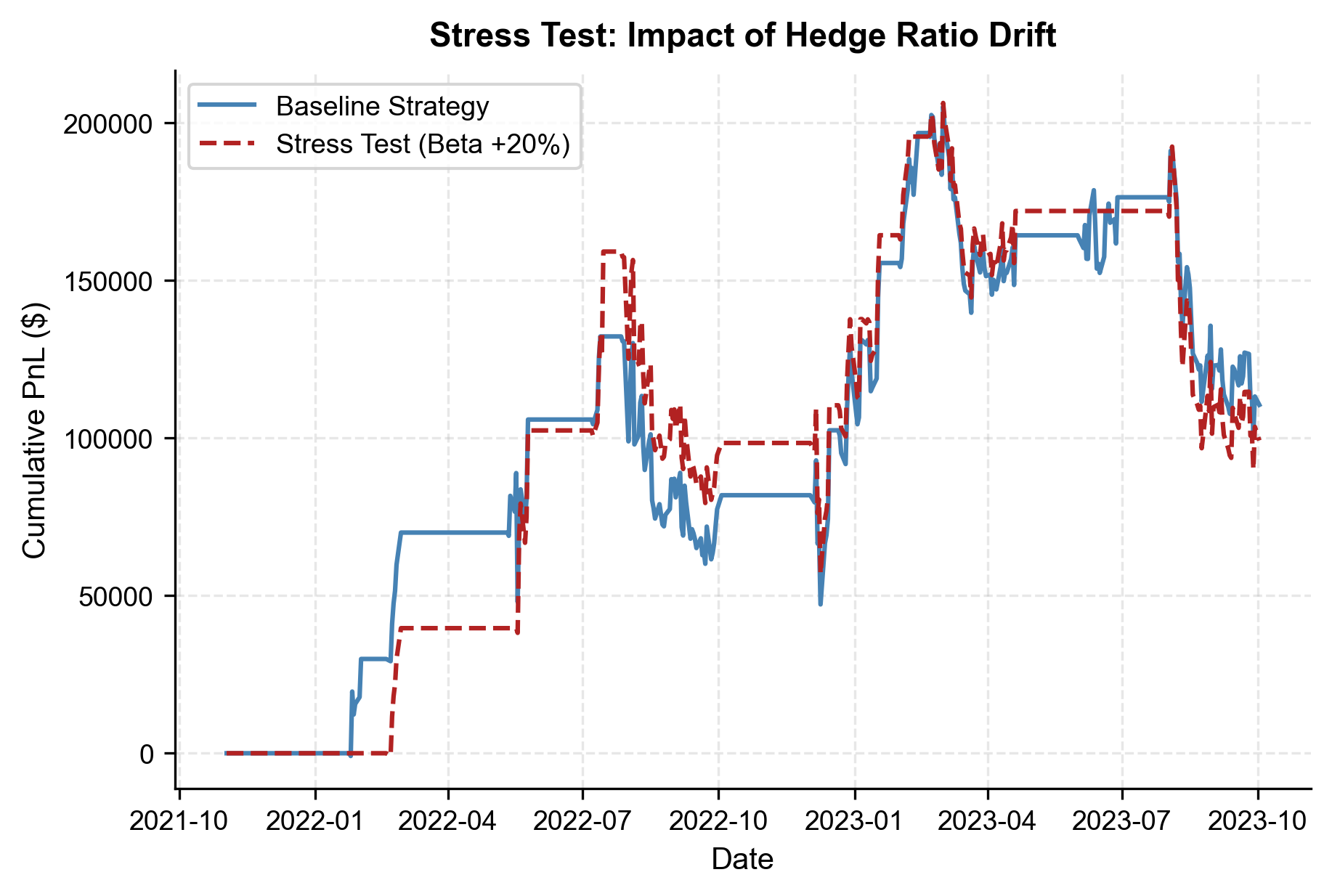
Stress Testing
Beyond standard risk metrics, we should ask: what happens if the cointegrating relationship breaks down? This is the primary tail risk for any pairs trading strategy. The standard risk metrics we computed above, VaR, CVaR, and maximum drawdown, all assume that the future will resemble the recent past. Stress testing relaxes this assumption by deliberately introducing adverse scenarios that may not appear in the historical data but are plausible based on economic reasoning.
For a pairs trading strategy, the most dangerous scenario is a structural shift in the hedge ratio. This can occur when one company in the pair undergoes a fundamental change: a merger announcement, a major product launch, a regulatory action, or a shift in business mix. When the true hedge ratio changes but our model continues to use the old estimate, the spread we compute no longer represents a stationary, mean-reverting quantity. Instead, it drifts systematically, generating false signals that lead to losses.
We simulate a scenario where the hedge ratio shifts by 20% midway through the test period.
The stress test reveals how sensitive the strategy is to parameter drift, a real-world risk that underscores the importance of periodically re-estimating the hedge ratio in production.
Summary of Risk Controls
A deployable strategy needs explicit risk controls documented in advance. Here is the risk framework for our pairs strategy:
- Position-level stop-loss. Close the position if the z-score exceeds . This limits losses from structural breaks.
- Position sizing. Risk no more than half-Kelly per trade, subject to a hard cap of 2% of capital.
- Portfolio-level limits. If running multiple pairs, cap gross exposure at 200% of capital and net exposure at 20%.
- Hedge ratio re-estimation. Re-estimate every 60 trading days using rolling regression. If the ADF p-value on the new spread exceeds 0.10, halt trading the pair until cointegration is re-established.
- Daily VaR limit. If the 1-day 95% VaR exceeds 1% of portfolio NAV, reduce position sizes proportionally.
Stage 7: Deployment Readiness
With a backtested strategy and risk framework in place, we now outline what it takes to move from research to live trading. This draws on the infrastructure and execution concepts from the earlier chapters in this part.
System Architecture
A pairs trading strategy requires several interconnected components:
- Data ingestion. Real-time price feeds for both stocks, with a fallback to delayed data for monitoring. Store tick-level and minute-bar data for execution; daily closes for signal generation.
- Signal engine. Compute the spread, rolling z-score, and position signal at the close of each trading day (or intraday if operating at higher frequency). This is the code we developed above, wrapped in a production framework.
- Order management system (OMS). Translate position changes into orders. For a pairs trade, this means simultaneously sending a buy order for one leg and a sell order for the other, ideally using a pairs execution algorithm that minimizes leg risk (the risk that one leg fills and the other does not).
- Risk monitor. Continuously track exposure, PnL, drawdown, and VaR against limits. Generate alerts when thresholds are approached.
- Reconciliation. At end-of-day, reconcile fills from the broker against the strategy's internal position records. Any discrepancies must be flagged and resolved.
Execution Considerations
As we discussed in the chapters on transaction costs and execution algorithms, the way we execute trades has a material impact on realized performance:
- Leg risk. In a pairs trade, both legs must be executed simultaneously. Using a single exchange and limit-order approach creates the risk that only one side fills. Market orders guarantee execution but at the cost of wider spreads. Smart execution algorithms balance these trade-offs, as covered in the optimal execution chapter.
- Market impact. Our backtest assumed 10 basis points of round-trip costs, which is reasonable for liquid large-cap equities. For smaller stocks or larger position sizes, slippage could be significantly higher.
- Execution timing. We generate signals at market close and execute at the next day's open. The overnight gap between signal and execution introduces slippage. An alternative is to trade near the close using a VWAP or TWAP algorithm.
Monitoring and Decay Detection
Once live, the most important ongoing task is monitoring for strategy decay. Mean-reverting strategies can stop working when:
- The fundamental linkage between the two stocks weakens (e.g., one company diversifies into a new business line).
- Market conditions shift such that mean reversion gives way to momentum (e.g., during a sector-wide trend driven by macro factors).
- Other market participants discover and trade the same pair, arbitraging away the opportunity.
We implement a simple monitoring framework by tracking the rolling Sharpe ratio and the ADF test p-value on the live spread.
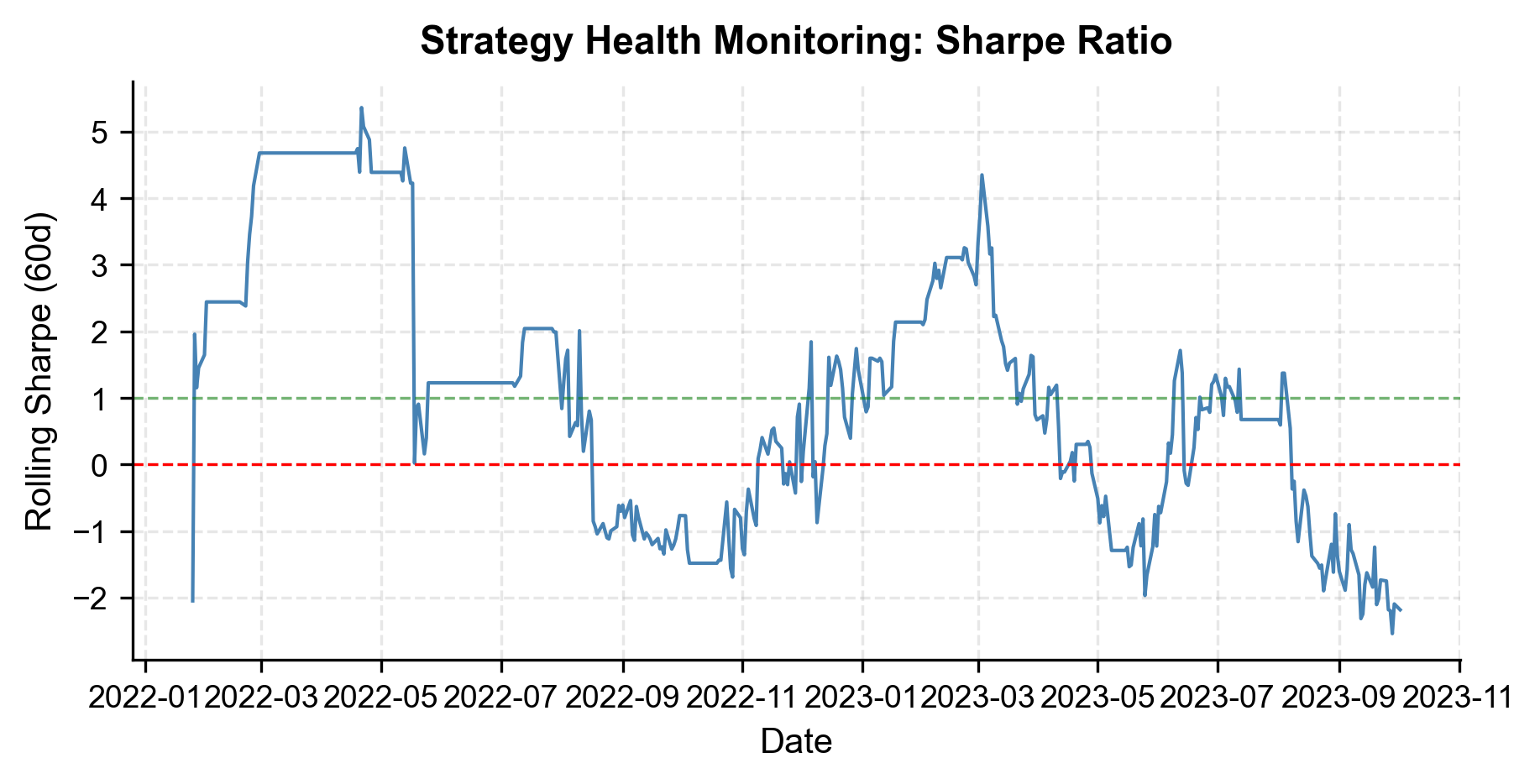
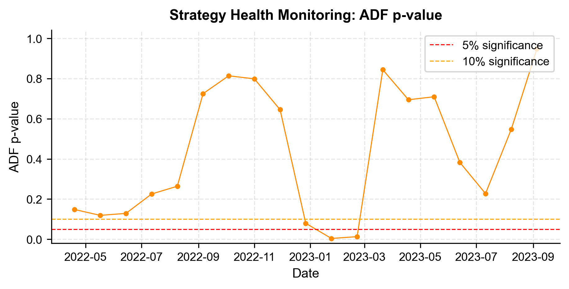
The monitoring dashboard gives us an at-a-glance view of strategy health. If the rolling Sharpe drops below zero for an extended period or the ADF p-value rises above 0.10, these are early warning signs that the cointegrating relationship is weakening, and we should consider pausing the strategy and re-evaluating.
Pre-Deployment Checklist
Before going live, you should work through a comprehensive checklist that spans everything covered in Part VII:
- Backtest validation. Is the out-of-sample performance consistent with in-sample? Are the assumptions (transaction costs, fill rates, data quality) realistic?
- Risk limits defined. Position size, stop-loss, portfolio-level exposure, and daily loss limits are documented and coded into the system.
- Execution tested. Has the execution algorithm been tested in a paper trading environment? Is leg risk controlled?
- Infrastructure resilient. Are there failover mechanisms for data feeds, execution gateways, and signal computation? What happens if the system goes down mid-day?
- Regulatory compliance. Are short-selling restrictions accounted for? Is the strategy compliant with market manipulation rules, as we discussed in the ethics chapter?
- Monitoring automated. Are alerts configured for drawdown limits, VaR breaches, and cointegration breakdown?
- Kill switch. Is there a manual override to flatten all positions immediately?
Key Parameters
The key parameters for the pairs trading strategy are:
- Lookback (): Window size (60 days) for rolling statistics used to normalize the spread.
- Entry Threshold (): Z-score magnitude (2.0) triggering trade entry.
- Exit Threshold (): Z-score magnitude (0.5) triggering trade exit.
- Stop-Loss (): Z-score magnitude (3.5) triggering forced exit to limit losses.
- Hedge Ratio (): The ratio of Stock A shorted for every unit of Stock B bought (or vice versa).
- Transaction Cost: 10 bps round-trip cost assumed for modeling slippage and commissions.
Limitations and Practical Considerations
This case study, while comprehensive in its process, intentionally simplifies several dimensions that would matter in production. The most significant limitation is our use of synthetic data. Real financial data presents challenges that synthetic data cannot replicate: earnings announcements that cause discrete jumps in the spread, short-selling constraints that make one leg more expensive to maintain, and periods of market stress where correlations spike and cointegration relationships temporarily break down. In practice, pair selection itself is a challenging problem: with stocks, there are possible pairs to test, creating a severe multiple comparison problem that inflates the false discovery rate. Bonferroni or Benjamini-Hochberg corrections should be applied when scanning for cointegrated pairs, but even these cannot fully protect against overfitting.
Another key limitation is parameter stability. We estimated a single hedge ratio from the training period and used it throughout the test period. In reality, hedge ratios drift over time as companies evolve, and a static will gradually become stale. More sophisticated implementations use Kalman filters or rolling regressions to dynamically update the hedge ratio, at the cost of introducing additional parameters that must themselves be tuned. The strategy also assumes continuous market access and the ability to short sell without constraints, neither of which is guaranteed. Short-selling costs (borrow fees) can be substantial for hard-to-borrow stocks and should be modeled explicitly. Finally, our transaction cost model of 10 basis points round-trip is a rough approximation; real costs depend on order size, time of day, market volatility, and the specific execution algorithm used, all topics we covered in the transaction costs and execution chapters.
Despite these limitations, the framework we built, with its strict train-test separation, explicit risk controls, and monitoring infrastructure, represents the disciplined approach that separates quantitative research from gambling. The specific numbers matter less than the process.
Summary
This chapter tied together the full arc of the textbook by building a pairs trading strategy from scratch. The key takeaways are:
- Start with economic rationale. Every strategy needs a clear reason why the pattern should exist and persist. For pairs trading, the rationale is rooted in common factor exposure and arbitrage forces that push temporarily divergent prices back toward equilibrium.
- Validate statistically before trading. We used the Engle-Granger cointegration test to confirm our hypothesis before committing capital. Statistical validation, using the time series tools from Part III, separates disciplined research from data mining.
- Backtest rigorously with out-of-sample data. The in-sample/out-of-sample split is non-negotiable. We estimated all model parameters (hedge ratio, intercept) on training data and evaluated performance on unseen data, incorporating realistic transaction costs.
- Integrate risk management from the start. Stop-losses, position sizing via the Kelly criterion, VaR monitoring, and stress testing are not afterthoughts. They are integral to the strategy design, drawing on the risk management principles from Part V and the position sizing framework from Part VII.
- Plan for deployment and decay. A strategy is only useful if it can be executed in production. We outlined the system architecture, execution considerations, and monitoring framework needed to run the strategy live, and defined explicit criteria for when to pause or retire it.
The strategy we built is deliberately simple. In practice, you would layer on additional sophistication: dynamic hedge ratio estimation, multi-pair portfolio construction, regime detection, and more granular execution modeling. But the process, from idea through validation through deployment, remains the same regardless of complexity. Mastering this process is what makes you a quantitative trader, not just a programmer who happens to work with financial data.
Quiz
Ready to test your understanding? Take this quick quiz to reinforce what you've learned about building a quantitative pairs trading strategy.

Comments