Router Z-Loss › Implementation
 Language AI HandbookAll chapters
Router Z-Loss › ImplementationOne section · Sections in this chapter8 / 12 ↓
Reading tools Definitions & inline links
Choose your expertise level to adjust how many terms are explained. Beginners see more tooltips, experts see fewer to maintain reading flow. Hover over underlined terms for instant definitions.
Article links
Make inline references clickable
Let's implement z-loss and observe its effect on router behavior. We'll build on the MoE infrastructure from previous chapters.
import numpy as np
import torch

# Set seeds for reproducibility
torch.manual_seed(42)
np.random.seed(42)
Z-Loss Computation
The core z-loss computation follows directly from the mathematical definition. The implementation is simple precisely because PyTorch's logsumexp function handles the numerically stable computation internally, applying the max-subtraction trick automatically.
def compute_z_loss(router_logits: torch.Tensor) -> torch.Tensor:
    """
    Compute router z-loss to encourage small logit magnitudes.

    Args:
        router_logits: Tensor of shape (batch_size, num_experts)
                      containing raw router logits before softmax

    Returns:
        Scalar z-loss value
    """
    # Compute log-sum-exp for each token (numerically stable)
    # logsumexp automatically handles the max-subtraction trick
    log_sum_exp = torch.logsumexp(router_logits, dim=-1)  # (batch_size,)

    # Square and average across batch
    z_loss = torch.mean(log_sum_exp**2)

return z_loss# Test z-loss on different logit scales
small_logits = torch.randn(32, 8) * 1.0 # Standard normal scale
medium_logits = torch.randn(32, 8) * 5.0 # 5x scale
large_logits = torch.randn(32, 8) * 20.0 # 20x scale
# Compute losses for display
loss_small = compute_z_loss(small_logits)
loss_medium = compute_z_loss(medium_logits)
loss_large = compute_z_loss(large_logits)Z-loss values for different logit scales: Small logits (std=1.0): 6.4938 Medium logits (std=5.0): 53.8352 Large logits (std=20.0): 1251.4348
The z-loss increases substantially with logit scale. This provides strong incentive to keep logits bounded. Notice the roughly quadratic scaling: the medium logits have a standard deviation 5x larger than the small logits, and their z-loss is roughly 25x larger.

Router with Z-Loss
Now let's create a router class that computes both routing probabilities and the z-loss. The key design principle is to compute z-loss on the raw logits, before any softmax or top-k selection. Computing z-loss after softmax would be mathematically incorrect, as the softmax output is already a probability distribution bounded between 0 and 1, which cannot exhibit the logit drift we are trying to prevent.
import torch
import torch.nn as nn
import torch.nn.functional as F


def compute_z_loss(router_logits: torch.Tensor) -> torch.Tensor:
    """
    Compute router z-loss to encourage small logit magnitudes.

    Args:
        router_logits: Tensor of shape (batch_size, num_experts)
                      containing raw router logits before softmax

    Returns:
        Scalar z-loss value
    """
    # Compute log-sum-exp for each token (numerically stable)
    # logsumexp automatically handles the max-subtraction trick
    log_sum_exp = torch.logsumexp(router_logits, dim=-1)  # (batch_size,)

    # Square and average across batch
    z_loss = torch.mean(log_sum_exp**2)

    return z_loss


class RouterWithZLoss(nn.Module):
    """Router network that tracks z-loss for stability."""

    def __init__(self, hidden_dim: int, num_experts: int):
        super().__init__()
        self.num_experts = num_experts
        self.gate = nn.Linear(hidden_dim, num_experts, bias=False)

        # Initialize with small weights to start with small logits
        nn.init.normal_(self.gate.weight, std=0.01)

    def forward(self, x: torch.Tensor, top_k: int = 2):
        """
        Compute routing probabilities and z-loss.

        Args:
            x: Input tensor of shape (batch_size, hidden_dim)
            top_k: Number of experts to select

        Returns:
            routing_weights: Top-k routing probabilities (batch_size, top_k)
            expert_indices: Selected expert indices (batch_size, top_k)
            z_loss: Scalar z-loss for this batch
        """
        # Compute router logits
        logits = self.gate(x)  # (batch_size, num_experts)

        # Compute z-loss before any masking
        z_loss = compute_z_loss(logits)

        # Get routing probabilities
        routing_probs = F.softmax(logits, dim=-1)

        # Select top-k experts
        top_k_probs, top_k_indices = torch.topk(routing_probs, top_k, dim=-1)

        # Renormalize top-k probabilities
        top_k_weights = top_k_probs / top_k_probs.sum(dim=-1, keepdim=True)

        return top_k_weights, top_k_indices, z_loss
Visualizing Z-Loss Effects
Let's visualize how z-loss affects logit distributions during training. The simulation below introduces a "task loss" that deliberately encourages larger logit magnitudes, mimicking the natural logit drift that occurs in real MoE training. We then compare training runs with different z-loss coefficients to see how the regularization contains this drift.
import torch


def simulate_training_step(router, optimizer, inputs, z_loss_coeff):
    """Simulate one training step with z-loss."""
    optimizer.zero_grad()

    # Forward pass
    weights, indices, z_loss = router(inputs)

    # Simulated task loss: penalise low-confidence routing (encourages the
    # router to produce larger logit magnitudes, mimicking the logit-drift
    # pressure seen in real language-model training).
    logits = router.gate(inputs)
    task_loss = -logits.abs().mean()

    # Combined loss
    total_loss = task_loss + z_loss_coeff * z_loss

    # Backward pass
    total_loss.backward()
    optimizer.step()

    return z_loss.item()


def run_training_simulation(z_loss_coeff: float, steps: int = 100):
    """Run training simulation tracking z-loss and logit statistics."""
    hidden_dim = 64
    num_experts = 8
    batch_size = 32

    torch.manual_seed(0)
    router = RouterWithZLoss(hidden_dim, num_experts)
    optimizer = torch.optim.Adam(router.parameters(), lr=0.05)

    z_losses = []
    max_logits = []
    mean_logits = []

    for step in range(steps):
        # Generate random inputs
        inputs = torch.randn(batch_size, hidden_dim)

        # Get current logit statistics before training step
        with torch.no_grad():
            logits = router.gate(inputs)
            max_logits.append(logits.abs().max().item())
            mean_logits.append(logits.abs().mean().item())

        # Training step
        z_loss = simulate_training_step(router, optimizer, inputs, z_loss_coeff)
        z_losses.append(z_loss)

return z_losses, max_logits, mean_logits# Run simulations to compare different z-loss coefficients
coefficients = [0.0, 0.05, 0.5]
results = {}
for coeff in coefficients:
z_losses, max_logits, _ = run_training_simulation(coeff, steps=100)
results[coeff] = {"z_losses": z_losses, "max_logits": max_logits}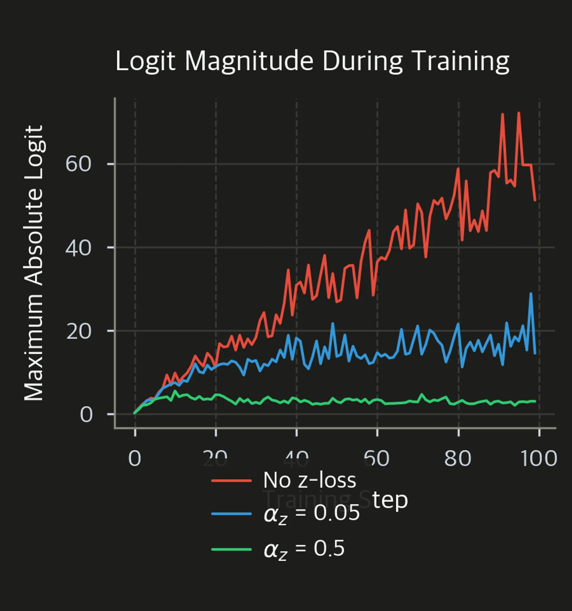

Without z-loss, the logit magnitudes grow freely. With z-loss applied, the optimizer continuously pushes logits back toward smaller values, establishing a stable equilibrium. The strength of the equilibrium is controlled by the coefficient: a larger coefficient produces a lower equilibrium logit magnitude, at the cost of potentially over-constraining the router.
Complete MoE with Combined Losses
Let's implement a complete MoE layer that computes both load balancing and z-loss. This implementation mirrors what you would find in production MoE systems, combining the two auxiliary loss terms in a single forward pass.
import torch
import torch.nn as nn
import torch.nn.functional as F


class MoELayerWithAuxLosses(nn.Module):
    """
    Mixture of Experts layer with both load balancing and z-loss.
    """

    def __init__(
        self,
        hidden_dim: int,
        num_experts: int = 8,
        expert_dim: int = 256,
        top_k: int = 2,
        aux_loss_coeff: float = 0.01,
        z_loss_coeff: float = 0.001,
    ):
        super().__init__()
        self.num_experts = num_experts
        self.top_k = top_k
        self.aux_loss_coeff = aux_loss_coeff
        self.z_loss_coeff = z_loss_coeff

        # Router
        self.router = nn.Linear(hidden_dim, num_experts, bias=False)
        nn.init.normal_(self.router.weight, std=0.01)

        # Expert networks (simple FFN for illustration)
        self.experts = nn.ModuleList(
            [
                nn.Sequential(
                    nn.Linear(hidden_dim, expert_dim),
                    nn.GELU(),
                    nn.Linear(expert_dim, hidden_dim),
                )
                for _ in range(num_experts)
            ]
        )

        # Track auxiliary losses
        self.aux_loss = 0.0
        self.z_loss = 0.0

    def compute_load_balancing_loss(
        self, router_probs: torch.Tensor, expert_mask: torch.Tensor
    ) -> torch.Tensor:
        """Compute auxiliary load balancing loss."""
        # Fraction of tokens routed to each expert
        tokens_per_expert = expert_mask.float().mean(dim=0)

        # Average routing probability per expert
        router_prob_per_expert = router_probs.mean(dim=0)

        # Load balancing loss (encourage uniform distribution)
        aux_loss = self.num_experts * torch.sum(
            tokens_per_expert * router_prob_per_expert
        )

        return aux_loss

    def forward(self, x: torch.Tensor) -> torch.Tensor:
        """
        Forward pass with auxiliary loss computation.

        Args:
            x: Input tensor of shape (batch_size, seq_len, hidden_dim)

        Returns:
            Output tensor of same shape as input
        """
        batch_size, seq_len, hidden_dim = x.shape
        x_flat = x.view(-1, hidden_dim)  # (batch_size * seq_len, hidden_dim)

        # Router forward pass
        router_logits = self.router(x_flat)  # (B*S, num_experts)
        router_probs = F.softmax(router_logits, dim=-1)

        # Compute z-loss
        self.z_loss = compute_z_loss(router_logits)

        # Select top-k experts
        top_k_probs, top_k_indices = torch.topk(
            router_probs, self.top_k, dim=-1
        )

        # Create expert mask for load balancing loss
        expert_mask = torch.zeros_like(router_probs)
        expert_mask.scatter_(1, top_k_indices, 1.0)

        # Compute load balancing loss
        self.aux_loss = self.compute_load_balancing_loss(
            router_probs, expert_mask
        )

        # Renormalize top-k weights
        top_k_weights = top_k_probs / top_k_probs.sum(dim=-1, keepdim=True)

        # Compute expert outputs (simplified loop implementation)
        output = torch.zeros_like(x_flat)
        for i in range(self.top_k):
            expert_idx = top_k_indices[:, i]  # (B*S,)
            weight = top_k_weights[:, i : i + 1]  # (B*S, 1)

            for e in range(self.num_experts):
                mask = expert_idx == e
                if mask.any():
                    expert_input = x_flat[mask]
                    expert_output = self.experts[e](expert_input)
                    output[mask] += weight[mask] * expert_output

        return output.view(batch_size, seq_len, hidden_dim)

    def get_total_aux_loss(self) -> torch.Tensor:
        """Get combined auxiliary loss for training."""
        return (
            self.aux_loss_coeff * self.aux_loss
            + self.z_loss_coeff * self.z_loss
)# Test the complete MoE layer
moe = MoELayerWithAuxLosses(
hidden_dim=128,
num_experts=8,
expert_dim=256,
top_k=2,
aux_loss_coeff=0.01,
z_loss_coeff=0.001,
)
# Sample input
x = torch.randn(4, 16, 128) # (batch, seq_len, hidden)
# Forward pass
output = moe(x)
# Extract values for display
input_shape = x.shape
output_shape = output.shape
load_balancing_loss = moe.aux_loss
z_loss_val = moe.z_loss
total_aux_loss = moe.get_total_aux_loss()Input shape: torch.Size([4, 16, 128]) Output shape: torch.Size([4, 16, 128]) Load balancing loss: 2.0054 Z-loss: 4.3186 Total auxiliary loss: 0.0244
The model processes the input shape [4, 16, 128] and produces a matching output shape, confirming that the MoE layer is dimensionality-preserving. The auxiliary losses are non-zero, showing that both balancing and z-loss constraints are active and adding to the training objective.
Monitoring Auxiliary Losses
During training, tracking both auxiliary losses helps diagnose issues. The monitoring approach below logs all four relevant quantities: task loss, load balancing loss, z-loss, and total loss. This gives you a complete picture of how each component is evolving and whether any component is dominating the optimization unexpectedly.
import torch
import torch.nn.functional as F


def training_loop_with_monitoring(
    model: MoELayerWithAuxLosses,
    num_steps: int = 200,
    batch_size: int = 8,
    seq_len: int = 32,
    hidden_dim: int = 128,
):
    """Simulated training loop with loss monitoring."""
    optimizer = torch.optim.AdamW(model.parameters(), lr=1e-3)

    history = {"task_loss": [], "aux_loss": [], "z_loss": [], "total_loss": []}

    for step in range(num_steps):
        optimizer.zero_grad()

        # Generate random batch
        x = torch.randn(batch_size, seq_len, hidden_dim)
        target = torch.randn(batch_size, seq_len, hidden_dim)

        # Forward pass
        output = model(x)

        # Task loss (MSE for illustration)
        task_loss = F.mse_loss(output, target)

        # Combined loss
        aux_loss = model.get_total_aux_loss()
        total_loss = task_loss + aux_loss

        # Backward pass
        total_loss.backward()
        optimizer.step()

        # Record history
        history["task_loss"].append(task_loss.item())
        history["aux_loss"].append(model.aux_loss.item())
        history["z_loss"].append(model.z_loss.item())
        history["total_loss"].append(total_loss.item())

return history# Train the model
moe = MoELayerWithAuxLosses(
hidden_dim=128,
num_experts=8,
expert_dim=256,
top_k=2,
aux_loss_coeff=0.01,
z_loss_coeff=0.001,
)
history = training_loop_with_monitoring(moe, num_steps=200)


The auxiliary losses quickly reach stable values while the task loss continues to improve. This is the desired behavior: the routing constraints are satisfied early and maintained throughout training. This provides a stable foundation for the task learning to proceed.
Expert Load Distribution
We can also track how the auxiliary losses affect expert utilization. This analysis runs the trained model on many random batches and counts how often each expert is selected across all tokens, giving a picture of whether the load balancing objective has achieved its goal.
import torch
import torch.nn.functional as F


def analyze_expert_distribution(
    model: MoELayerWithAuxLosses, num_samples: int = 100
):
    """Analyze expert load distribution after training."""
    model.eval()

    expert_counts = torch.zeros(model.num_experts)
    total_tokens = 0

    with torch.no_grad():
        for _ in range(num_samples):
            x = torch.randn(8, 32, 128)
            x_flat = x.view(-1, 128)

            router_logits = model.router(x_flat)
            router_probs = F.softmax(router_logits, dim=-1)
            _, top_k_indices = torch.topk(router_probs, model.top_k, dim=-1)

            for k in range(model.top_k):
                for e in range(model.num_experts):
                    expert_counts[e] += (top_k_indices[:, k] == e).sum()

            total_tokens += x_flat.shape[0] * model.top_k

    expert_fractions = expert_counts / total_tokens
return expert_fractions.numpy()expert_fractions = analyze_expert_distribution(moe)
The combined effect of load balancing loss and z-loss produces well-distributed expert utilization, close to the ideal uniform distribution. This confirms that the two auxiliary losses are working as intended: z-loss maintains numerical stability while load balancing ensures all experts are actively used.