Router Z-Loss › Z-Loss Formulation

Router z-loss directly penalizes large logit magnitudes by adding a regularization term to the training objective. Rather than placing hard constraints on logit values, which would require constrained optimization techniques, z-loss uses soft regularization that integrates smoothly with standard gradient descent. The formulation targets the log-sum-exp of router logits, a smooth, differentiable proxy for the maximum logit that has particularly nice mathematical properties.

The design of z-loss reflects several important engineering considerations. Hard constraints like "no logit may exceed value X" are difficult to enforce efficiently in distributed training and create discontinuous gradients at the constraint boundary. Penalty terms on individual logits (such as L2 regularization) apply pressure uniformly, which can interfere with the router's ability to develop discriminative patterns. Z-loss avoids both problems: it is smooth, it automatically focuses pressure on the largest logits, and it is trivial to compute alongside the standard softmax.

Think of z-loss as a built-in pressure release valve. As logits grow, the penalty grows even faster (quadratically), creating an increasing counterforce that slows the drift before it causes problems. This is analogous to a thermostatic system: when the temperature rises above a comfortable level, the cooling mechanism kicks in harder, establishing a stable equilibrium rather than letting unbounded temperature increase.

Router z-loss directly penalizes large logit magnitudes by adding a regularization term to the training objective. Rather than placing hard constraints on logit values, which would require constrained optimization techniques, z-loss uses soft regularization that integrates smoothly with standard gradient descent. The formulation targets the log-sum-exp of router logits, a smooth, differentiable proxy for the maximum logit that has particularly nice mathematical properties.

For a batch of $B$ tokens, where token $i$ has router logits $z_{i,j}$ for expert $j$, the z-loss is defined as:

$$\mathcal{L}_z = \frac{1}{B} \sum_{i=1}^{B} \left( \log \left( \sum_{j=1}^{N} \exp(z_{i,j}) \right) \right)^2$$

where:

• $\mathcal{L}_z$: the router z-loss
• $B$: the batch size (number of tokens)
• $N$: the number of experts
• $z_{i,j}$: the logit for token $i$ and expert $j$
• $\log \sum \ldots$: the log-sum-exp term approximating the maximum logit

Let's unpack this formula to understand how it works. The innermost part, $\sum_{j=1}^{N} \exp(z_{i,j})$, computes the sum of exponentials of all logits for a single token. This sum is exactly the normalization constant that appears in the denominator of the softmax function. Taking the logarithm of this sum gives us the log-sum-exp (LSE), which has a natural interpretation as a "soft maximum" of the logits.

The inner term $\log \sum_j \exp(z_{i,j})$ is the log-sum-exp (LSE) of the logits for token $i$. This function has a useful property that makes it ideal for our purposes: it approximates the maximum logit while remaining smooth and differentiable everywhere:

$$\max_j z_{i,j} \leq \log \sum_{j=1}^{N} \exp(z_{i,j}) \leq \max_j z_{i,j} + \log N$$

where:

• $\max_j z_{i,j}$: the largest logit value for token $i$, representing the router's most confident assignment
• $N$: the total number of experts in the layer
• $\log N$: a constant upper bound on the approximation error, roughly 2.1 for 8 experts or 4.2 for 64 experts

Why does this formula make sense? Notice that when one logit $z_{i,k}$ dominates all others by a large margin, $\sum_j \exp(z_{i,j}) \approx \exp(z_{i,k})$, so $\log \sum_j \exp(z_{i,j}) \approx z_{i,k} = \max_j z_{i,j}$. The approximation is tight when the routing is confident. When all logits are equal, the sum is $N \cdot \exp(z)$ and the log-sum-exp equals $z + \log N$, which is exactly $\log N$ above the maximum. So the bound holds with equality at both extremes.

This inequality tells us that the LSE always lies between the maximum logit and the maximum logit plus $\log N$. For typical expert counts (8, 16, or 64 experts), $\log N$ is a small constant (approximately 2.1, 2.8, or 4.2 respectively), so the LSE closely tracks the maximum logit. However, unlike the hard maximum function, which has discontinuous gradients at points where multiple logits are tied, the LSE is smooth everywhere. This smoothness is important for gradient-based optimization.

Squaring this quantity and averaging across tokens creates a penalty that grows quadratically as logits increase. The squaring operation has two important effects: it ensures the loss is always non-negative, and it provides increasingly strong regularization as logits grow. A token with LSE value of 10 contributes 100 to the loss, while a token with LSE value of 20 contributes 400. This quadratic growth creates strong pressure to keep logits bounded without overly penalizing moderate values.

The log-sum-exp formulation has several advantages over alternative approaches to constraining logit magnitudes. These advantages show why this design has become standard in MoE training rather than simpler alternatives:

• Smooth gradients: Unlike penalties on $\max_j z_j$ (which has discontinuous gradients at points where the maximum switches from one logit to another) or $\sum_j z_j^2$ (which penalizes all logits equally regardless of their relative magnitudes), LSE smoothly emphasizes the largest logits while giving gradients to all experts. When one logit is much larger than the others, the LSE gradient is concentrated on that logit. When multiple logits are similar, the gradient is distributed among them. This smooth interpolation between these cases makes optimization well-behaved and prevents the abrupt gradient changes that occur with hard maximum penalties.

• Scale awareness: The LSE naturally captures the "effective scale" of the logit distribution in a way that considers both the maximum value and the spread. For example, a distribution with logits $[10, 10, 10]$ has an LSE of approximately $11.1$, while a distribution with logits $[30, 30, 30]$ has an LSE of approximately $31.1$. Although both produce identical uniform probability distributions (and thus have the same entropy), their LSE values differ significantly, correctly which reflects that the larger logits pose greater stability risks. This is precisely the behavior we want: penalizing scale independently of routing patterns.

• Numerical stability: The LSE is itself computed stably using the max-subtraction trick, avoiding the very overflow issues we are trying to prevent. Modern deep learning frameworks implement numerically stable versions of log-sum-exp that never overflow, making z-loss reliable to compute even when logits have already drifted to large values. This means z-loss can be applied as a corrective measure even when training has already started experiencing instability.

• Computational efficiency: The LSE is already computed as an intermediate result during the softmax calculation. In practice, the numerator $\sum_j \exp(z_{i,j})$ appears in the softmax denominator, and the LSE is just the log of this quantity. Frameworks like PyTorch's torch.logsumexp implement this without additional overhead, making z-loss essentially free to compute in terms of wall-clock time.

An alternative approach one might consider is simply applying L2 regularization directly to the router weights $W_r$. This would prevent the weights from growing large, which would indirectly bound logit magnitudes. The problem with this approach is that weight decay applies pressure uniformly to all router weights, including those that are small and produce benign logits. Z-loss, by contrast, applies pressure specifically proportional to the current logit magnitudes, putting correction where it is most needed while leaving well-behaved logits largely undisturbed.

To understand the effect of z-loss on training dynamics, we derive its gradient with respect to the router logit $z_{i,j}$. This derivation reveals how the loss creates corrective pressure on large logits and why the pressure is proportional to both the current scale and the routing confidence.

The gradient we want to compute answers the question: if logit $z_{i,j}$ increases by a small amount, how does the z-loss change? A large gradient means z-loss strongly penalizes further increases in this logit. This provides a restoring force. A small gradient means z-loss is nearly indifferent to this logit. This allows it to change freely.

Applying the chain rule to the squared term:

$$\begin{aligned} \frac{\partial \mathcal{L}_z}{\partial z_{i,j}} &= \frac{\partial}{\partial z_{i,j}} \left[ \frac{1}{B} \sum_{k=1}^{B} \text{LSE}(z_k)^2 \right] \\ &= \frac{1}{B} \cdot \frac{\partial}{\partial z_{i,j}} (\text{LSE}(z_i)^2) && \text{(only term $i$ depends on $z_{i,j}$)} \\ &= \frac{1}{B} \cdot 2 \cdot \text{LSE}(z_i) \cdot \frac{\partial}{\partial z_{i,j}} \text{LSE}(z_i) && \text{(power rule)} \\ &= \frac{2}{B} \cdot \text{LSE}(z_i) \cdot \text{softmax}(z_i)_j && \text{(derivative of LSE is softmax)} \end{aligned}$$

where:

• $\frac{\partial \mathcal{L}_z}{\partial z_{i,j}}$: the gradient of the loss with respect to a specific logit
• $B$: the batch size
• $\text{LSE}(z_i)$: the log-sum-exp value for token $i$
• $\text{softmax}(z_i)_j$: the probability assigned to expert $j$

The key insight in this derivation is that the derivative of the log-sum-exp with respect to one of its inputs is exactly the corresponding softmax probability. This elegant relationship emerges from the structure of the exponential function and is a standard result in mathematical statistics. Formally, if $\text{LSE}(z) = \log \sum_j \exp(z_j)$, then $\frac{\partial \text{LSE}}{\partial z_j} = \frac{\exp(z_j)}{\sum_k \exp(z_k)} = \text{softmax}(z)_j$.

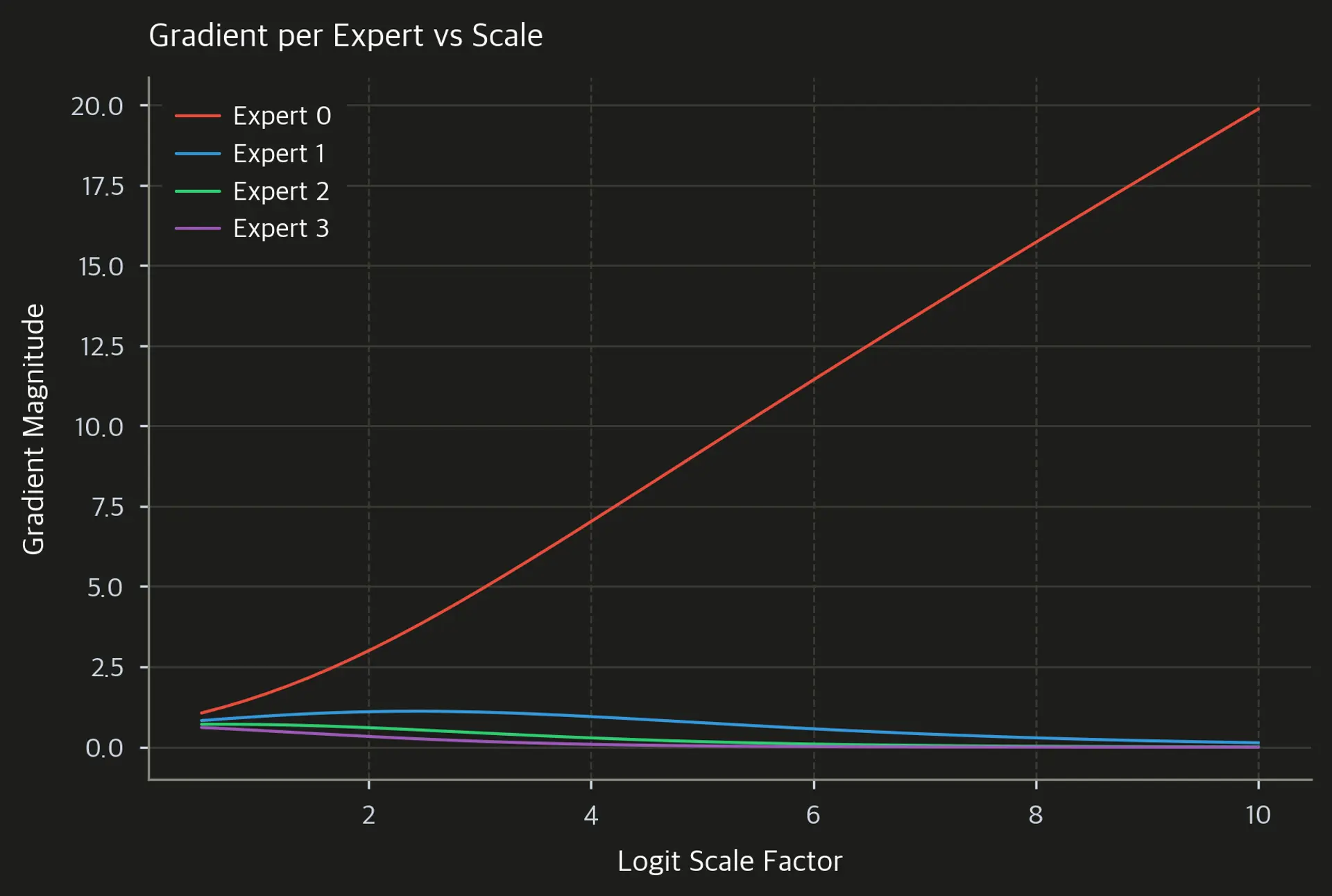
Why does this formula make sense? Notice that the gradient has exactly two factors multiplied together: the current LSE value (representing the "scale emergency severity") and the softmax probability (representing "which logit is most responsible for the high scale"). The product naturally directs corrective pressure where it is most needed. When the LSE is small, the gradient is small, meaning z-loss barely touches the router when logits are healthy. When the LSE grows large, the gradient scales up proportionally. This provides increasingly aggressive correction. This self-calibrating behavior is what makes z-loss an effective regularizer rather than a blunt instrument.

This gradient formula reveals important behavior that explains why z-loss is effective:

• The gradient is proportional to the current softmax probability: experts receiving more routing get larger gradients pushing their logits down. This is exactly what we want, as the experts with the largest logits (and therefore highest probabilities) receive the strongest corrective signal. Experts that are already receiving little routing probability receive only small gradients from z-loss, letting them to remain available for future routing without being artificially suppressed.

• The gradient scales with the current LSE value: larger logits create stronger corrective pressure. When the LSE is small (showing well-behaved logits), the z-loss gradient is correspondingly small and doesn't interfere much with task learning. When the LSE grows large (showing potential instability), the gradient grows proportionally, creating a stronger restoring force.

• The quadratic nature (from squaring) provides increasingly strong regularization as logits grow. The factor of 2 from the power rule, combined with the LSE scaling, means the gradient grows faster than linearly with logit magnitude. This provides gentle regularization for moderate logits but strong correction for extreme values, striking a balance between letting useful routing patterns and preventing numerical instability.