Part of Language AI Handbook
Route LLM requests intelligently across model tiers using rule-based, difficulty-based, and cascade strategies, plus A/B testing to validate routing decisions.
Choose your expertise level to adjust how many terms are explained. Beginners see more tooltips, experts see fewer to maintain reading flow. Hover over underlined terms for instant definitions.
Article links
Make inline references clickable
Model Routing
When you deploy a language model into production, you rarely have just one model. A modern production system might run a small 7B-parameter model alongside a 70B model and a frontier API like GPT-4 or Claude. The challenge is deciding which model should handle which request. Route everything to the big model and your costs explode. Route everything to the small model and quality suffers. Model routing is the discipline of making that decision intelligently: matching each request to the most appropriate model based on its complexity, cost constraints, latency requirements, and expected difficulty.
To appreciate why this matters, consider the economics of inference. Frontier models like GPT-4 or Claude cost roughly 10 to 50 times more per token than a well-tuned 7B open-source model. If you have 100,000 daily requests, even routing 70% of them to the cheaper tier while maintaining comparable quality on easy tasks can translate to 60-70% cost reductions. At scale, that difference often determines whether a product is economically viable.
This chapter covers model routing methods, including simple rule-based selection, learned routing classifiers, A/B tests for routing decisions, and cascaded systems that escalate requests through increasingly capable (and expensive) models. We also examine the tradeoffs between different routing strategies and the operational challenges of running routed systems at scale.
Why Routing Matters
A single model cannot simultaneously minimize latency, maximize quality, and minimize cost. These goals are in direct tension:
- Larger models produce higher quality outputs but require more memory, take longer to respond, and cost more per token to run.
- Smaller models respond quickly and cheaply but may struggle with complex reasoning, instructions with subtle constraints, or specialized domains.
- Specialized models excel in their domain but fail outside it.
Routing resolves this tension by treating the model selection itself as a decision problem. Instead of picking one model for all traffic, you build a system that dynamically assigns each request to the model best suited for it.
The economic advantage follows from the traffic mix. Suppose 80% of your traffic consists of simple factual lookups or short responses that a 7B model handles correctly, while only 20% requires deep reasoning that demands a 70B model. A naive system that routes everything to the 70B model pays full cost for all requests. A well-calibrated router that correctly classifies that 80/20 split reduces inference costs by roughly 4x while maintaining overall quality. For a startup paying $50,000 per month on inference, that improvement drops the bill to $12,500 without changing the user experience.
Quality imposes the opposite constraint. You could cut costs by routing everything to the cheapest model, but that sacrifices quality on the hard requests your users care most about. Routing lets you invest inference budget where it matters: applying heavy computational resources precisely where simpler models would fail.
A third motivation is latency. Users notice when responses take longer than two seconds. A small model that responds in 100 milliseconds delivers a fundamentally different user experience than a large model that takes three seconds. Routing short, straightforward queries to the fast small model while reserving the slower large model for complex tasks lets you hit latency targets that no single model can consistently achieve.
Model routing is a system that directs incoming requests to different model backends based on estimated task complexity, cost constraints, latency requirements, or domain. The goal is to use the cheapest model that can produce acceptable quality for each specific request.
What Makes a Request Hard?
Before building a router, you need a working theory of what makes some requests harder than others. No single observable feature answers this question reliably.
Request difficulty correlates with several observable signals. Long requests with complex multi-step instructions tend to require more reasoning than short factual questions. Requests that ask the model to synthesize information from multiple domains, construct structured outputs (like code or JSON), or perform mathematical reasoning are systematically harder than requests that ask for straightforward retrieval. Requests involving ambiguous pronouns, implicit context, or domain-specific terminology challenge models that lack that context.
But the correlation is imperfect. A single-sentence question like "What is the integral of ?" is short but difficult. A paragraph-long request asking for a simple rewrite might be trivially easy. Length, vocabulary, and structural complexity are proxies for difficulty, not direct measurements of it. Any routing system built on proxies will make mistakes, and understanding where those mistakes cluster is essential for improving the system over time.
The most principled definition of difficulty is relative to the models available: a request is "hard" for a given model tier if that tier's output quality falls below an acceptable threshold. This makes difficulty a property of the request-model pair, not the request alone. The same question that stumps a 7B model may be trivially answered by a 70B model. This insight motivates the cascade architecture, where difficulty is evaluated dynamically rather than predicted statically.
Routing Strategies
Routing strategies span a wide range, from completely static rules to fully learned systems that adapt to incoming data. The right choice depends on your system's complexity, latency budget, and how much signal you have about request difficulty.
Rule-Based Routing
The simplest routing strategy uses deterministic rules to partition traffic. These rules operate on observable request features without any machine learning:
- Request length: Short requests (under 50 tokens) go to the small model; long requests go to the large model.
- Keyword matching: Requests containing technical keywords from a domain-specific vocabulary are routed to a specialized model.
- User tier: Premium users get the larger model; free-tier users get the smaller one.
- Time of day: Route to cheaper models during peak hours to control costs; use the better model during off-peak periods.
- Explicit task type: Requests beginning with "summarize" or "translate" may be handled reliably by a smaller model, while requests asking for "explain step by step" or "write code to" might be escalated automatically.
Rule-based routing is easy to implement, inspect, and debug. There are no training data requirements and no risk of distributional shift in the router itself. The rules are transparent: every routing decision can be traced to a specific condition, which matters in regulated industries or when debugging quality regressions.
The downside is brittleness. Rules cannot capture the full complexity of what makes a request hard. A short request can require sophisticated reasoning. A long request might be a simple document with repetitive structure. Rules drawn from proxy features like length or keywords will misclassify these cases systematically. As your product evolves, you accumulate exceptions, special cases, and workarounds that make the rule set increasingly fragile. A request that was easy six months ago may require the large model today because the task has grown more demanding with your user base.
Rule-based routing works best as a starting point, not a final destination. It establishes a baseline from which you can measure improvements as you gather data and build more sophisticated classifiers.
Difficulty-Based Routing
A more principled approach estimates task difficulty directly. Difficulty-based routers learn a mapping from request features to a difficulty score, then threshold that score to select a model tier.
The intuition is that request difficulty is often predictable from surface features: the type of question (factual vs. reasoning), the domain (general vs. specialized), the presence of multi-step instructions, the required output format, or historical patterns for similar queries.
A difficulty classifier can be trained on labeled data where each request has an associated quality label from each model tier. A request is "hard" if the small model fails but the large model succeeds. This creates a supervised learning problem: predict whether a given request will cause the small model to fail.
The classifier can be as simple as a logistic regression over a small feature vector, or as complex as a fine-tuned language model that reads the request and outputs a difficulty score. In practice, the classifier needs to be much faster than the models it routes between, which pushes toward lightweight approaches. A gradient-boosted tree trained on a hundred features can make a routing decision in under a millisecond. A fine-tuned 1B-parameter model might take 50 milliseconds, which is acceptable if you are routing between a 500ms small model and a 5,000ms large model, but not if you are routing between a 30ms and a 200ms model.
The challenge is acquiring labeled data. You can bootstrap it by running a sample of traffic through all model tiers simultaneously, collecting outputs, and using human evaluation or an automated judge to compare quality. This is expensive initially but creates a feedback loop that improves the router over time. Each new labeled example makes the difficulty classifier more accurate, which in turn makes routing decisions better, which produces clearer signals for the next round of evaluation.
One of the most useful single-feature difficulty proxies is the perplexity of the request under the small model itself. Perplexity measures how surprised the model is by the input text: low perplexity means the model has seen similar patterns frequently, while high perplexity indicates unfamiliar content. A request that the small model assigns high perplexity is more likely to be outside its training distribution and therefore more likely to produce a poor response. Computing perplexity is fast (a single forward pass, no generation required) and provides a continuous difficulty signal.
Cost-Aware Routing
Cost-aware routing explicitly incorporates economic constraints into the routing decision. Rather than picking a model purely on predicted quality, it maximizes a utility function that weighs expected quality against expected cost.
For a request , the routing decision selects model from a set of available models :
where:
- : the expected quality score for request handled by model
- : the expected cost of routing request to model
- : a cost-quality tradeoff parameter that controls how aggressively to prefer cheaper models
This formulation makes the tradeoff explicit. A high routes aggressively to cheaper models; a low prioritizes quality. In practice, can be tuned globally or adjusted dynamically based on remaining budget for the billing period.
The elegance of this formulation is that it handles multi-tier decisions naturally. With three or more model tiers, you do not need separate rules for each pair. The optimizer considers all available models and selects whichever maximizes the utility function. You can add a new model tier without restructuring the entire routing logic, simply by adding it to with its cost and quality estimates.
One important subtlety is that must be estimated before routing, not measured after. You do not know the actual quality of model 's response to request until you generate it. In practice, is a predicted expected quality, estimated from features of and historical quality data for model . This prediction introduces uncertainty: if the quality estimate is noisy, the routing decision may be suboptimal. Systems that track prediction confidence can handle this by routing to the larger model when quality estimates are uncertain, essentially treating uncertainty as a signal to be cautious.
Dynamic adjustment is an important practical feature. Early in a billing cycle, when budget is ample, you might set low to prioritize quality. As you approach the end of the cycle, increases, pushing more traffic to cheaper models. This gives operators direct control over the cost-quality tradeoff as a function of budget state.
Embedding-Based Routing
Embedding-based routers represent each incoming request as a vector in a shared embedding space and use similarity to previously seen requests (with known routing outcomes) to decide where to route the new request.
The approach works as follows. When a request arrives, you compute its embedding using a lightweight encoder. You then look up its nearest neighbors in a database of historical requests with known outcomes (quality scores from each model). If similar requests were handled well by the small model, you route there. If similar requests required the large model, you escalate.
This approach captures semantic similarity that keyword rules miss. A new question about Riemannian geometry that you have never seen before may share semantic space with previous calculus questions that the small model handled poorly. Embedding-based routing can generalize from a small number of labeled examples to handle novel requests gracefully because it uses continuous vector similarity rather than discrete rule matching.
The tradeoff is latency: the embedding computation and nearest-neighbor lookup add overhead on every request. For systems with strict latency budgets, this overhead may be prohibitive unless the lookup is highly optimized. Approximate nearest-neighbor algorithms like FAISS or HNSW make the lookup fast enough for practical use: retrieving the top-k neighbors from a database of a million vectors takes under 5 milliseconds on modern hardware.
Another limitation is the cold start problem. Embedding-based routing requires a sufficiently large and diverse database of labeled examples to generalize well. A sparse database with only a few dozen examples will not cover the request distribution adequately, and the nearest-neighbor matches will be unreliable. This makes embedding-based routing more suitable as a mature-phase routing strategy, once you have accumulated substantial labeled data, rather than a system you deploy on day one.
Learned Routing Classifiers
A learned routing classifier trains a lightweight model specifically to predict which backend model should handle a given request. This is typically a binary or multi-class classifier:
- Binary: "Should this request go to the small model or the large model?"
- Multi-class: "Which of these five model tiers should handle this request?"
The classifier inputs are typically lightweight features derived from the request: token counts, perplexity under a small language model, POS tag distributions, presence of domain keywords, or embeddings from a small encoder. The output is a routing decision.
The key design principle is that the classifier must be much cheaper than the models it routes between. A classifier that takes 50ms to make a routing decision saves nothing if it prevents a 30ms call to the small model. Practical routing classifiers are typically small linear models, gradient-boosted trees, or compact neural networks with inference times under 5ms.
Training data for the classifier comes from historical routing outcomes. Each training example consists of a feature vector derived from the request and a label indicating which model tier produced acceptable quality. This creates a natural label definition: if the small model's quality score exceeded threshold on a given request, label it "small"; otherwise label it "large." The classifier learns to predict this label from request features without ever seeing the model responses at routing time.
One practical consideration is class imbalance. If 80% of your requests are easy (small model is sufficient), the classifier will see four times as many positive examples as negative ones. Standard techniques for handling class imbalance apply: reweighting the loss function, oversampling the minority class, or using calibrated probability outputs with a decision threshold adjusted to reflect the desired escalation rate.
Model Cascades
A model cascade is a sequential routing architecture where requests are processed by a cheap model first, and only escalated to more expensive models if the cheap model's output is deemed insufficient. This is sometimes called "progressive evaluation" or "cost-aware inference."
The fundamental difference from upfront routing classifiers is the direction of information flow. A routing classifier decides before generating any response. A cascade generates a response first and then decides whether that response is good enough. This allows the cascade to use the actual model output, including its confidence and uncertainty, as evidence for the escalation decision. You are not predicting whether the model will fail; you are observing whether it failed and acting accordingly.
A model cascade is a routing architecture that processes each request starting with the cheapest available model and escalates to more capable (and expensive) models only when a confidence check determines the current model's output is insufficient.
Cascade Architecture
A two-tier cascade works as follows. When a request arrives, the small model generates a response. An evaluator then assesses the small model's confidence or output quality. If the evaluator judges the output acceptable, it is returned to the user. If not, the request is forwarded to the large model, which generates its own response. The large model's output is returned as the final answer.
The evaluator is the critical component. Common evaluation strategies include:
- Self-confidence: The small model outputs a probability or confidence score with its response. Responses below a threshold are escalated.
- Proxy judge: A separate lightweight model evaluates the small model's output quality.
- Semantic uncertainty: Methods that estimate how uncertain the model is, such as measuring the entropy of the output distribution or generating multiple samples and measuring their variance.
- Factual consistency checks: For structured outputs, automated checks can verify whether the response satisfies basic constraints (valid JSON, correct format, required fields present). A response that fails these checks is escalated without further evaluation.
The quality of the cascade depends entirely on the quality of the evaluator. A poor evaluator that keeps low-quality outputs from the small model will degrade end-to-end quality, while an overly conservative evaluator that escalates everything will eliminate the cost savings. The evaluator is where most of the engineering effort in a cascade system goes.
Notice that a cascade imposes an inherent latency penalty on escalated requests. When the large model eventually handles a request, the system has already paid for the small model's generation plus the evaluator's assessment. The total latency for an escalated request is the sum of small model latency, evaluator latency, and large model latency. This means cascades are most economically efficient when a large fraction of requests are handled at the first tier and only a small minority escalate.
Confidence Thresholds
The most common cascade evaluator uses the model's own confidence as a proxy for output quality. For classification tasks, this is straightforward: if the model's maximum class probability exceeds a threshold , return the response. Otherwise, escalate.
For generative tasks, confidence estimation is harder. Language models do not naturally output a single confidence score for a free-form generated response. Common proxies include:
- Token-level log probability: The sum or mean of log probabilities assigned to the generated tokens. Low log probability suggests the model is uncertain about its own output. The mean log probability per token, sometimes called the average negative log-likelihood, is particularly useful because it normalizes for response length, allowing fair comparison across responses of different lengths.
- Entropy of the first token distribution: High entropy on the first generated token often correlates with overall response uncertainty. This signal is especially cheap to compute because you only need a single forward pass to the first generation step, not the full response.
- Self-consistency: Generate responses from the small model and measure agreement. If diverse samples agree on the key facts or conclusion, the model is likely confident. High variance across samples signals uncertainty.
The self-consistency approach is particularly powerful for reasoning tasks. For a question with a single correct answer, generating five samples and checking whether they all agree provides a stronger confidence signal than any single probability score. A model that answers "42" five times out of five is almost certainly correct. A model that produces five different answers signals uncertainty. The downside is cost: generating samples multiplies the small model cost by , which only makes sense if .
For each of these proxies, you select a threshold by calibrating on a validation set with known quality labels. The threshold trades off between:
- Escalation rate: The fraction of requests forwarded to the large model (directly determines cost).
- Quality coverage: The fraction of requests where the small model's output meets quality requirements.
This tradeoff has a characteristic shape. At very low thresholds, almost nothing escalates: you accept every small model response, quality is whatever the small model can produce, and cost is minimized. As you raise the threshold, more requests escalate, quality improves because you are catching the small model's worst outputs, but cost increases. At very high thresholds, almost everything escalates regardless of actual quality, and your cascade degenerates into always-large routing. The optimal threshold sits somewhere in the middle, depending on your quality requirements and budget.
Selecting the threshold requires a validation set with ground-truth quality labels. You sweep the threshold from 0 to 1, compute the quality-cost curve, and select the threshold that satisfies your quality constraint at minimum cost, or that maximizes quality given a cost budget. This calibration step is not optional. An uncalibrated threshold is as likely to hurt you as help you.
Multi-Tier Cascades
The cascade concept extends naturally to more than two tiers. A three-tier system might use a 7B model, then a 70B model, then a frontier API. Each tier applies its confidence check; only requests that exceed the escalation threshold at tier are forwarded to tier .
The cost model for a -tier cascade is:
where:
- : the cost per request for model tier
- : the probability that a request reaches tier
For a well-calibrated cascade, (all requests hit tier 1), and for each subsequent tier (fewer and fewer requests escalate). If 80% of requests are resolved at tier 1, 15% at tier 2, and 5% at tier 3, you pay for 100% of requests, for 20%, and for 5%.
With realistic cost ratios (e.g., , , ), the expected cost is units, compared to units if everything went to tier 3. That is a 12.5x cost reduction for the same end-to-end quality on the 80% of requests handled at tier 1.
Multi-tier cascades become progressively harder to calibrate. Each tier needs its own confidence estimator tuned to detect the specific failure modes of that tier's model. The thresholds interact: setting tier 1's threshold too low offloads requests to tier 2 that would have been fine, and they may not escalate further to tier 3 even if they should. This interdependency means you generally need to calibrate thresholds jointly rather than independently.
A practical simplification is to treat each tier's evaluator as independent and tune thresholds greedily: first optimize tier 1's threshold to minimize the number of easy requests that escalate while catching the cases where tier 1 fails, then optimize tier 2's threshold similarly for requests that reach it. This greedy approach does not find the global optimum but is much more tractable and works well in practice.
When Cascades Underperform
Cascades are not universally superior to upfront routing. There are several scenarios where they underperform.
When the small model is very slow, the latency penalty from always running the small model first may be unacceptable. If your small model takes 300 milliseconds and your large model takes 800 milliseconds, an escalated request takes over a second just for the small model's wasted inference. Users will notice.
When the escalation evaluator is weakly calibrated, the cascade may produce worse quality than either a good upfront classifier or always using the large model. A bad evaluator that fails to detect low-quality small model outputs produces an end-to-end system that silently degrades.
When almost all requests need the large model (high inherent difficulty distribution), a cascade wastes the cost of running every request through the small model first. If 80% of requests will escalate, the small model run is pure overhead.
Understanding these failure modes helps you decide when to use a cascade versus a routing classifier. A routing classifier is better when you have good upfront signals about difficulty. A cascade is better when difficulty is hard to predict before generation but easy to assess after.
A/B Testing for Routing Decisions
A/B testing is the standard method for evaluating whether a routing strategy improves outcomes. Without rigorous A/B testing, it is easy to believe a routing improvement is real when it is just noise, or to miss an improvement because the measurement methodology was flawed.
The stakes are high. Routing changes can silently degrade quality for a subset of users without triggering any obvious error signals. Unlike a bug that causes crashes, a routing policy that routes 5% of hard requests to the weak model manifests as a small quality drop that is easy to rationalize as noise. Rigorous A/B testing is the discipline that separates real improvements from wishful thinking.
Experimental Design
An A/B test for model routing compares two routing strategies:
- Control (A): The current routing policy, typically a single model or an existing routing rule.
- Treatment (B): The new routing policy being evaluated.
Incoming requests are randomly split between the two strategies. The split must be random at the request level to ensure statistical independence. Splitting by user (all requests from a given user go to the same strategy) helps detect personalization effects but requires careful analysis to account for user-level confounders. User-level splitting is appropriate when routing decisions interact with user history or when the quality of a response depends on prior responses in the same session.
Key metrics to measure:
- Quality: Measured by human evaluation, automated scoring, or task-specific metrics (BLEU, accuracy, etc.)
- Latency: P50, P90, and P99 latencies for each strategy
- Cost per request: Total inference cost divided by request count
- Escalation rate (for cascades): Fraction of requests reaching each tier
The choice of quality metric deserves careful attention. Automated metrics are cheap and scalable but may not align with what users care about. Human evaluation is expensive but provides ground truth. A common hybrid is to use automated metrics for continuous monitoring and human evaluation for final decision-making. The automated metric should be validated against human judgments before you trust it to make routing decisions.
Latency metrics require percentile reporting, not just mean latency. Mean latency is heavily influenced by slow outliers and can mask important patterns. A routing strategy that reduces mean latency by 10% while increasing P99 latency by 50% is not an improvement from a user experience perspective. P99 latency determines the worst experience users encounter in normal operation.
Statistical Significance
A/B test results should not be trusted until they achieve statistical significance. For quality metrics scored as continuous values, a two-sample -test compares means. For binary quality metrics (pass/fail), a proportion test or chi-squared test is appropriate.
The minimum detectable effect (MDE) depends on sample size, variance, and the significance threshold . For a routing test where quality improvements may be small (1-2%), large sample sizes are needed. A useful rule of thumb: if your daily traffic is requests and you split 50/50, you need approximately:
where:
- : the critical value for significance level (for , )
- : the variance of the quality metric
- : the minimum effect size you want to detect
At and (2% quality improvement) with , you need roughly 1,700 samples per arm. A system with 10,000 daily requests could complete this test in under a day. A system with 100 daily requests would need three weeks.
This formula highlights a real tension for early-stage products. You cannot get fast feedback on routing quality until you have substantial traffic. This is one reason routing systems are typically deployed later in a product's lifecycle, after traffic has grown enough to support rapid experimentation.
Multiple testing is another concern. If you run many routing experiments simultaneously, some will appear significant by chance. The Bonferroni correction reduces each experiment's significance threshold by the number of simultaneous tests. A system running five experiments simultaneously at should apply a per-experiment threshold of to maintain the family-wise error rate. In practice, most routing systems run sequential rather than simultaneous experiments, which reduces but does not eliminate this concern.
Guardrails
A/B tests for routing policies need guardrails to prevent harm during the test. If the treatment strategy is dramatically worse, you want to detect this quickly and stop the experiment. Common guardrails include:
- Early stopping rules: Stop the experiment if quality metrics fall below a threshold in the treatment arm. Sequential testing methods like the Bonferroni-corrected sequential probability ratio test (SPRT) allow you to stop early with controlled error rates.
- Sample size caps: Limit the fraction of traffic exposed to the treatment arm (e.g., 5% treatment, 95% control) until initial results are promising. A bad treatment only harms 5% of users until you have confidence it is safe.
- Real-time monitoring: Watch latency and error rate dashboards during the test to catch operational issues immediately. A treatment strategy that introduces unexpected model calls or failures should be caught by alerting before it reaches statistical significance.
- Novelty filters: Ensure the test traffic is representative. If your treatment arm accidentally receives more hard requests due to non-random assignment, the apparent quality drop is confounded with traffic composition, not causally related to the routing strategy.
Holdout Groups and Long-Running Tests
Some routing improvements take time to evaluate properly. If a new routing strategy routes certain users more consistently to the large model, those users may notice a quality improvement and engage more deeply with the product, which affects long-term metrics like retention and satisfaction. These effects are invisible in a short A/B test.
A holdout group is a permanently held-out fraction of traffic (typically 5-10%) that receives the baseline strategy even after the new strategy has been rolled out to everyone else. This allows long-term comparison of users who experienced the new strategy versus those who did not. Holdout groups are standard practice at large tech companies for exactly this reason: they catch effects that short experiments miss.
For routing systems specifically, holdout groups help measure whether routing improvements that look good on immediate quality metrics also improve downstream outcomes like task completion rate, follow-up request rate, or user satisfaction scores.
Routing in Practice
Understanding routing strategies conceptually is one thing; implementing them reliably in a production system requires careful attention to engineering details.
Feature Engineering for Routing
The quality of a learned router depends heavily on the features it uses to represent incoming requests. Useful features include:
- Length features: Token count, word count, sentence count, average sentence length. These are cheap to compute and carry useful signal, even if imperfect.
- Linguistic features: Part-of-speech distributions, presence of questions, imperative phrases, or list structures. Requests with multiple embedded questions tend to be harder than single-question requests.
- Domain signals: TF-IDF scores against domain-specific corpora, keyword presence from domain vocabularies. A request containing dense mathematical notation is likely harder than a request about everyday topics.
- Complexity proxies: Perplexity of the request under a small language model (higher perplexity often correlates with harder requests), sentence embedding norms, or vocabulary richness measured by type-token ratio.
- Historical context: Whether similar requests in recent history were handled well by the small model, user-specific routing history.
- Structural features: Whether the request contains code, lists, mathematical expressions, or URLs. Requests that ask for code generation consistently require more capability than plain text requests.
Importantly, all these features must be computed quickly. If feature extraction takes 50ms, it dominates the latency budget for requests that are correctly routed to the 30ms small model. Feature engineering is a constant balance between predictive power and computational cost.
One practical technique is a two-level feature hierarchy. A first level of very cheap features (token count, simple keyword flags, character-level statistics) makes a fast initial routing decision for the clear-cut cases: obviously short and simple requests go to the small model, obviously long and complex requests go to the large model. A second level of more expensive features (perplexity, embedding similarity) is applied only to the ambiguous middle cases. This tiered approach concentrates the expensive feature computation where it matters most.
Latency Budgets
Every routing system has a latency budget. The routing decision itself adds overhead to every request. For requests that end up at the small model, the router adds latency. For requests that end up at the large model, the routing overhead is negligible relative to the large model's response time.
The break-even point for a router is when the overhead it adds to fast requests is justified by the savings from correctly avoiding the slow model. If your small model takes 50ms and your large model takes 500ms, and your router takes 10ms, then:
- Fast requests: 50ms + 10ms = 60ms (20% overhead)
- Slow requests (without router): 500ms
- Slow requests (with router, correctly routed to large): 500ms + 10ms = 510ms (2% overhead)
The routing overhead is acceptable as long as the router correctly avoids the large model often enough to compensate. If the router adds 10ms but only routes 5% of requests away from the large model, it is not worth it.
When routing overhead is a concern, asynchronous precomputation can help. For user-facing applications with a chat interface, you can begin computing routing features (and even the routing decision) while the user is still typing, before the request is submitted. By the time the request arrives, the routing decision is already made. This effectively eliminates routing latency from the user-perceived path.
Another latency optimization is request batching. If you aggregate multiple requests and route them as a batch, the per-request overhead of feature computation and classifier inference is amortized across the batch. Batch routing is most applicable in offline or near-real-time settings, not in interactive applications where each request must be routed immediately.
Cold Start and Bootstrapping
A learned routing classifier requires training data, but you do not have routing outcome labels before you deploy the system. This is the cold start problem.
Common bootstrapping approaches:
- Shadow evaluation: Run both models on all requests without using their outputs to make decisions. Collect quality labels from human evaluation or an automated judge. Use this to build the initial training set for the router.
- Heuristic initialization: Deploy a rule-based router first. Use its routing decisions (imperfect as they are) as initial labels, then iterate as you collect better feedback.
- Offline datasets: If you have historical request data, run it through both models offline and use the results to train the initial router.
- Synthetic data: Generate labeled examples by constructing requests of known difficulty (simple retrieval questions, multi-step reasoning problems) and evaluating model quality on them. Synthetic data is imperfect but can bootstrap a router until real traffic data accumulates.
The cold start problem means that routing system quality improves over time as more labeled data accumulates. Designing the system to continuously collect routing outcome feedback is as important as the initial routing design. This requires an explicit feedback collection pipeline: after each response, log the model tier used, the request features, and some quality signal (user rating, task completion flag, LLM judge score). This logged data is the training set for future router improvements.
Feedback Loops and Online Learning
A static routing classifier degrades over time as request distributions shift. A user base that starts with simple questions may evolve to ask more complex ones. New product features may introduce request types the router has never seen. Domain terminology changes.
Online learning addresses this by continuously updating the routing classifier as new labeled data arrives. In its simplest form, this means periodically retraining the classifier on a sliding window of recent requests. More sophisticated systems use online gradient descent to update model weights in real time.
However, online learning introduces its own risks. A classifier that learns too quickly from recent data can overfit to short-term distribution shifts, becoming unstable. A sudden spike in hard requests (say, due to a marketing campaign that attracts expert users) should not permanently shift the router toward always routing to the large model. Careful learning rate selection and regularization are needed to balance adaptability against stability.
An intermediate approach is to retrain the classifier on a schedule (weekly or monthly) using a rolling window of labeled data, rather than updating continuously. This provides adaptation to long-term distribution shifts without the instability of real-time updates. The retrained classifier is validated on a held-out set before deployment to catch regressions.
Router Monitoring and Observability
A production routing system needs dedicated monitoring to remain healthy. The key signals to track are:
- Escalation rate trend: If escalation rate is steadily increasing over weeks, it suggests the small model is increasingly struggling with incoming requests. This may indicate distributional shift, model degradation, or a product change that is attracting harder queries.
- Per-tier quality distribution: Monitor quality scores separately for requests handled by the small model and the large model. If small model quality scores start declining without a corresponding change in escalation rate, the evaluator may be miscalibrated.
- Router accuracy on labeled samples: Periodically evaluate the router on a labeled holdout set. If accuracy declines, it is time to retrain.
- Cost per request over time: Sudden changes in average cost signal routing behavior changes that may not be intended.
- Latency by tier: Track latency distributions separately for small-model and large-model requests. This helps distinguish between routing overhead (affects all requests) and model latency changes (affects only one tier).
Good observability makes the difference between a routing system you trust and one you fear. Without it, you will discover problems from user complaints rather than from metrics dashboards.
Code Implementation
Let's implement the core components of a model routing system: a difficulty-based router, a confidence-threshold cascade, and an A/B test evaluation framework.
We start by installing required packages and setting up the simulation environment.
Simulating Requests and Models
We simulate a production environment with requests of varying difficulty and two model tiers with different quality and cost profiles.
@dataclass
class Request:
    """A single inference request with a ground-truth difficulty score."""

    text: str
    difficulty: float  # 0.0 (easy) to 1.0 (hard)
    tokens: int


@dataclass
class ModelResponse:
    """Response from a model tier."""

    output: str
    quality: float  # 0.0 to 1.0
    confidence: float  # model's self-reported confidence
    cost: float  # cost in arbitrary units
    latency_ms: float


def generate_requests(n: int) -> list[Request]:
    """Generate requests with a realistic difficulty distribution.

    Most requests are easy (right-skewed), with a long tail of hard ones.
    """
    difficulties = np.random.beta(a=1.5, b=4.0, size=n)  # skewed toward easy
    token_counts = (20 + difficulties * 200 + np.random.randn(n) * 20).astype(
        int
    )
    token_counts = np.clip(token_counts, 10, 500)
    requests = [
        Request(text=f"request_{i}", difficulty=float(d), tokens=int(t))
        for i, (d, t) in enumerate(zip(difficulties, token_counts))
    ]
    return requests


def small_model_response(req: Request) -> ModelResponse:
    """Simulate a small (cheap) model. Struggles on hard requests."""
    # Quality degrades on harder requests; small model is noisy
    base_quality = 0.9 - 0.7 * req.difficulty
    quality = float(np.clip(base_quality + np.random.randn() * 0.1, 0, 1))
    # Confidence is correlated with actual quality, but noisy
    confidence = float(np.clip(quality + np.random.randn() * 0.15, 0, 1))
    return ModelResponse(
        output="small_answer",
        quality=quality,
        confidence=confidence,
        cost=0.001 * req.tokens,
        latency_ms=10 + req.tokens * 0.2,
    )


def large_model_response(req: Request) -> ModelResponse:
    """Simulate a large (expensive) model. High quality across all difficulties."""
    base_quality = 0.97 - 0.15 * req.difficulty
    quality = float(np.clip(base_quality + np.random.randn() * 0.05, 0, 1))
    confidence = float(np.clip(quality + np.random.randn() * 0.05, 0, 1))
    return ModelResponse(
        output="large_answer",
        quality=quality,
        confidence=confidence,
        cost=0.01 * req.tokens,
        latency_ms=100 + req.tokens * 2.0,
)Generated 1000 requests Difficulty: mean=0.272, std=0.170 Tokens: mean=74.0
The simulated requests follow a realistic distribution: most are relatively easy (mean difficulty around 0.27), with a long tail of harder requests. The small model's quality degrades as difficulty increases, while the large model maintains high quality throughout. This asymmetry is the key structural fact that makes routing useful.
Rule-Based Router
Our first router uses a simple difficulty threshold based on request length as a proxy.
def rule_based_router(req: Request, token_threshold: int = 100) -> str:
    """Route based on token count as a proxy for difficulty."""
    if req.tokens <= token_threshold:
        return "small"
    return "large"


def evaluate_router(
    requests: list[Request],
    router: Callable[[Request], str],
    label: str,
) -> dict:
    """Evaluate a routing strategy and collect metrics."""
    results = []
    for req in requests:
        decision = router(req)
        if decision == "small":
            resp = small_model_response(req)
        else:
            resp = large_model_response(req)
        results.append(
            {
                "decision": decision,
                "quality": resp.quality,
                "cost": resp.cost,
                "latency_ms": resp.latency_ms,
            }
        )

    qualities = [r["quality"] for r in results]
    costs = [r["cost"] for r in results]
    latencies = [r["latency_ms"] for r in results]
    small_frac = sum(1 for r in results if r["decision"] == "small") / len(
        results
    )

    return {
        "label": label,
        "mean_quality": float(np.mean(qualities)),
        "mean_cost": float(np.mean(costs)),
        "mean_latency_ms": float(np.mean(latencies)),
        "small_model_fraction": float(small_frac),
        "total_cost": float(np.sum(costs)),
}Always Large: Mean quality: 0.9237 Mean cost: 0.74011 Mean latency: 248.0 ms Small model %: 0.0% Total cost: 740.11 Rule-Based (token): Mean quality: 0.8255 Mean cost: 0.47525 Mean latency: 140.6 ms Small model %: 60.5% Total cost: 475.25
The rule-based router routes a substantial fraction of requests to the small model, reducing total cost significantly. The quality drop is small because most short requests are easy. This illustrates the core value proposition: you pay less without sacrificing much quality. The token threshold of 80 was chosen somewhat arbitrarily; in a real system, you would calibrate this by sweeping thresholds and evaluating quality on a labeled validation set.
Cascade Router
Next, we implement a cascade that uses confidence thresholds to decide whether to escalate.
def cascade_router(req: Request, confidence_threshold: float = 0.75) -> dict:
    """Two-tier cascade: try small model first, escalate if confidence is low."""
    small_resp = small_model_response(req)
    if small_resp.confidence >= confidence_threshold:
        return {
            "decision": "small",
            "quality": small_resp.quality,
            "cost": small_resp.cost,
            "latency_ms": small_resp.latency_ms,
            "escalated": False,
        }
    # Escalate to large model
    large_resp = large_model_response(req)
    return {
        "decision": "large",
        "quality": large_resp.quality,
        "cost": small_resp.cost + large_resp.cost,  # paid for both
        "latency_ms": small_resp.latency_ms + large_resp.latency_ms,
        "escalated": True,
    }


def evaluate_cascade(
    requests: list[Request],
    confidence_threshold: float,
    label: str,
) -> dict:
    results = [cascade_router(req, confidence_threshold) for req in requests]
    qualities = [r["quality"] for r in results]
    costs = [r["cost"] for r in results]
    latencies = [r["latency_ms"] for r in results]
    escalation_rate = float(np.mean([r["escalated"] for r in results]))

    return {
        "label": label,
        "mean_quality": float(np.mean(qualities)),
        "mean_cost": float(np.mean(costs)),
        "mean_latency_ms": float(np.mean(latencies)),
        "escalation_rate": escalation_rate,
        "total_cost": float(np.sum(costs)),
}tau=0.50: quality=0.7674, cost=0.24381, escalation=16.0% tau=0.65: quality=0.8295, cost=0.41921, escalation=36.8% tau=0.75: quality=0.8734, cost=0.56904, escalation=56.0% tau=0.85: quality=0.9009, cost=0.67690, escalation=74.4% tau=0.95: quality=0.9148, cost=0.74571, escalation=86.5%
The cascade results show a clear tradeoff: higher confidence thresholds (requiring more certainty before returning the small model's answer) increase escalation rates and costs, but also improve quality. The right threshold depends on your quality requirements and cost budget. Notice that even at the highest threshold (), the cascade still costs less than always routing to the large model, because it correctly handles the clearly easy requests at the small model.
A/B Testing Framework
Now let's build a simple A/B testing framework to evaluate routing strategies with statistical rigor.
from scipy import stats


def run_ab_test(
    requests: list[Request],
    router_a: Callable[[Request], str],
    router_b: Callable[[Request], str],
    split_ratio: float = 0.5,
    seed: int = 0,
) -> dict:
    """Run an A/B test comparing two routing strategies."""
    rng = np.random.default_rng(seed)
    # Randomly assign each request to arm A or arm B
    assignments = rng.random(len(requests)) < split_ratio  # True = arm A

    arm_a_results = []
    arm_b_results = []

    for req, in_a in zip(requests, assignments):
        if in_a:
            decision = router_a(req)
            resp = (
                small_model_response(req)
                if decision == "small"
                else large_model_response(req)
            )
            arm_a_results.append(
                {
                    "quality": resp.quality,
                    "cost": resp.cost,
                    "latency_ms": resp.latency_ms,
                }
            )
        else:
            decision = router_b(req)
            resp = (
                small_model_response(req)
                if decision == "small"
                else large_model_response(req)
            )
            arm_b_results.append(
                {
                    "quality": resp.quality,
                    "cost": resp.cost,
                    "latency_ms": resp.latency_ms,
                }
            )

    a_quality = [r["quality"] for r in arm_a_results]
    b_quality = [r["quality"] for r in arm_b_results]

    # Two-sample t-test for quality difference
    t_stat, p_value = stats.ttest_ind(a_quality, b_quality)
    quality_lift = float(np.mean(b_quality) - np.mean(a_quality))

    return {
        "n_a": len(arm_a_results),
        "n_b": len(arm_b_results),
        "quality_a": float(np.mean(a_quality)),
        "quality_b": float(np.mean(b_quality)),
        "quality_lift": quality_lift,
        "t_statistic": float(t_stat),
        "p_value": float(p_value),
        "significant_at_05": bool(p_value < 0.05),
        "cost_a": float(np.mean([r["cost"] for r in arm_a_results])),
        "cost_b": float(np.mean([r["cost"] for r in arm_b_results])),
        "latency_a": float(np.mean([r["latency_ms"] for r in arm_a_results])),
        "latency_b": float(np.mean([r["latency_ms"] for r in arm_b_results])),
}A/B Test: Always Large (Control) vs Cascade tau=0.75 (Treatment) Sample sizes: n_A=473, n_B=527 Quality: A=0.9248, B=0.8497, lift=-0.0751 Cost: A=0.72780, B=0.52633 Latency: A=245.6ms, B=166.7ms t-statistic: 12.865 p-value: 0.0000 Significant at alpha=0.05: True
The A/B test quantifies exactly what we gain and lose by switching from always routing to the large model to using a cascade. A small quality drop at lower cost, with statistical significance determined by the p-value. Reading these results correctly requires looking at all metrics together: a statistically significant quality drop that is also economically meaningful requires a different decision than a statistically significant but practically negligible drop.
Visualizing the Cost-Quality Tradeoff

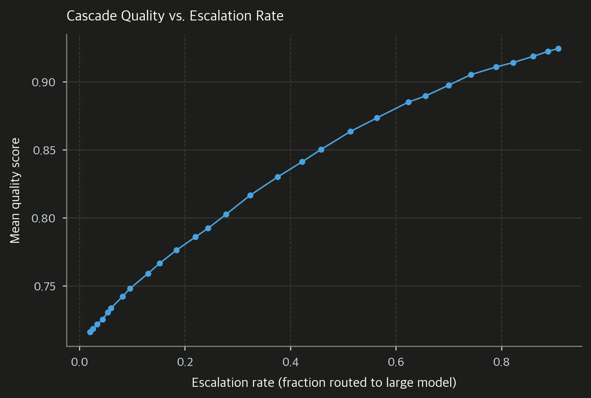
The escalation-quality curve captures an important practical insight: the marginal benefit of escalation changes across the operating range. Low-confidence requests tend to provide the largest early gains, while further escalation gradually approaches the always-large quality ceiling and continues to add cost. This means the optimal operating point is rarely "escalate everything uncertain" but rather "escalate until marginal quality gain equals marginal cost increase."


The quality comparison by difficulty bin reveals the core insight behind cascade routing: the models are closest on the easiest requests, while the small model's quality drops much faster as difficulty increases. This means the marginal value of escalation is concentrated in the high-difficulty tail. A good cascade exploits this by escalating only when it detects difficulty signals that predict poor small-model quality. Requests in the easy region can safely stay at the small model; the routing overhead on those requests is the price you pay for savings on the difficult ones.
Key Parameters
The key parameters for a cascade routing system are:
- confidence_threshold: The minimum confidence the small model must report to return its answer without escalation. Lower values route more to the small model (cheaper but lower quality); higher values escalate more frequently (better quality but higher cost).
- cost_ratio: The ratio of large model cost to small model cost per token. Determines how aggressively to optimize for the small model.
- escalation_cap: An optional maximum escalation rate, useful when you have a hard budget constraint. If your budget allows at most 20% of requests to reach the large model, set this cap explicitly rather than hoping the threshold happens to produce 20% escalation.
- routing_overhead_ms: The latency added by the routing decision itself. Must be small relative to the small model's response time to avoid negating the latency benefits of routing easy requests to the fast model.
Advanced Routing Architectures
The strategies described so far handle routing as a one-shot decision per request. Several more sophisticated architectures extend this foundation.
Speculative Execution
Speculative execution is a variant where the small model and large model run in parallel rather than sequentially. The large model begins generating a response at the same time as the small model. When the small model finishes, an evaluator assesses its output. If the small model's response is acceptable, the large model's generation is cancelled and the small model's response is returned. If not, the system waits for the large model to finish and returns its response.
This eliminates the latency penalty for escalated requests: instead of running small then large sequentially, the large model has been running the entire time. The cost penalty for speculation is the wasted large model compute on requests that ultimately did not need escalation. Speculation trades compute efficiency for latency guarantees.
The economic viability of speculative execution depends on the escalation rate and cost ratio. If 30% of requests escalate and the large model costs 10x the small model, then every 10 requests incurs the full large model cost for 10 requests but only 3 of them were necessary, wasting 7 large model runs. Whether this is worth the latency improvement depends on your latency requirements and cost budget.
Mixture-of-Routers
Rather than a single routing decision, some systems maintain multiple specialized routers, each tuned for a different request type, and use a meta-router to select which router to apply. A meta-router might first classify the request domain (code, math, creative writing, factual lookup), then apply a domain-specific routing policy that is calibrated for that domain's difficulty distribution.
This hierarchical approach works because difficulty is not uniform across domains. A 7B model might handle creative writing requests as well as a 70B model in most cases, but struggle with mathematical reasoning even for moderately difficult problems. Routing policies calibrated on all request types together will systematically under-route in some domains and over-route in others. Domain-specific policies correct for this.
The downside is complexity: you now have routing policies, where is the number of domains and is the number of model tiers. Maintaining, updating, and monitoring these policies scales linearly with the number of domains.
Budget-Constrained Routing
In production systems with hard cost budgets, routing policies must adapt dynamically to remaining budget. A system with a fixed monthly budget needs to be more conservative with the large model as the end of the month approaches.
Budget-constrained routing formalizes this by incorporating remaining budget directly into the routing decision. One approach modifies the cost-quality tradeoff parameter dynamically:
where is the total monthly budget, is the remaining budget at time , and is a base cost sensitivity. As budget is depleted, increases, pushing more traffic to the cheaper model. When budget is ample (early in the month), is low and the system prioritizes quality.
This creates a natural budget allocation strategy without requiring explicit planning. The system automatically becomes more conservative as constraints tighten, without any manual intervention.
Limitations and Practical Impact
Model routing introduces several failure modes that do not exist in single-model deployments. The most important is router miscalibration: if the routing classifier or confidence estimator is wrong, you either pay too much (routing easy requests to the large model) or sacrifice quality (routing hard requests to the small model). Neither failure is immediately visible in aggregate metrics without careful monitoring at the routing decision level. A quality degradation caused by systematic misrouting of a specific request type can easily be masked by the high quality on the majority of correctly routed requests.
The cold start problem is endemic to any system that learns from routing outcomes. You need labeled data to train the router, but you do not have labeled data until the system has been running. This creates a chicken-and-egg dependency. Practical systems solve this with a gradual rollout: start with a simple rule-based router, use shadow evaluation to collect quality labels, then train a more sophisticated classifier once you have enough data. The bootstrapping phase requires accepting suboptimal routing for weeks or months before the learned router is reliable enough to deploy.
Routing also creates complexity overhead that can slow iteration. A single-model system is easy to debug: if quality is bad, the model is bad. A routed system has multiple failure points: the router could be wrong, the small model could be degrading, the large model could have a different issue, or the confidence estimator could be miscalibrated. Operational teams need tooling to isolate which component is responsible for quality issues. This tooling investment is real and should be budgeted explicitly when planning a routing system.
A subtle failure mode is distributional shift in the routing classifier itself. If the request distribution changes, the classifier's learned boundaries between easy and hard requests may no longer be correct. A classifier trained when your user base consisted mostly of students may misroute the complex research questions that enter the distribution when you expand to professional users. Monitoring escalation rates and per-tier quality distributions provides early warning of this shift.
The interaction between routing and user experience creates another challenge. If users learn that reformulating their questions as shorter or simpler-sounding queries produces faster responses (because the system routes them to the small model), they may adapt their behavior to game the router. This creates a feedback loop where the distribution of "simple-looking but complex" requests increases over time, degrading router accuracy. This phenomenon, sometimes called Goodhart's Law applied to routing, is difficult to detect and correct.
Well-implemented model routing can reduce inference cost substantially with minimal quality loss. The greatest savings occur in applications with heavy-tailed request distributions: if most requests are easy, a cascade that handles 90% of traffic with the cheap model and escalates only the difficult 10% achieves near-large-model quality at near-small-model cost. This makes routing one of the production optimizations with the largest cost impact at scale.
From an industry perspective, the rise of routing systems reflects a broader maturation of LLM deployment. Early adopters simply called the best available API for every request. As costs became significant, teams began differentiating between request types. Now, sophisticated routing systems with multiple tiers, learned classifiers, and continuous calibration are standard practice at any organization running LLMs at scale. The companies that do this well gain a structural cost advantage that compounds over time as their routing data and models improve.
Summary
Model routing is the practice of directing inference requests to the most appropriate model based on estimated difficulty, cost constraints, and quality requirements. Key takeaways:
- Routing strategies range from deterministic rules (token length thresholds, user tiers) to learned classifiers that predict request difficulty from surface features, with cost-aware formulations that make the quality-cost tradeoff explicit and tunable.
- Model cascades implement a sequential approach: try the cheap model first, evaluate confidence, and escalate to a more capable model only when necessary. The confidence threshold controls the cost-quality tradeoff. The escalation-quality curve typically shows diminishing returns beyond 30-40% escalation rate.
- A/B testing is essential for validating routing decisions. Compare routing strategies with statistical rigor using appropriate sample sizes, significance thresholds, and guardrails against harmful treatments. Never trust a routing improvement without measuring it.
- Cold start is the primary operational challenge: learned routers require labeled routing outcome data that only exists after the system has been running. Bootstrapping through shadow evaluation or rule-based initialization is necessary.
- Routing overhead must be small relative to the small model's latency. Routers that are expensive to run negate their own savings. Practical classifiers operate in under 5ms.
- Online learning keeps routers up to date as request distributions shift, but requires careful regularization to avoid instability from short-term fluctuations.
- Observability is what separates routing systems you trust from ones you fear. Monitor escalation rate trends, per-tier quality distributions, and router accuracy on labeled holdout sets continuously.
Production routing systems demonstrate that significant cost savings are achievable without sacrificing quality, provided the routing decision is well-calibrated and continuously monitored. The engineering investment in building, calibrating, and maintaining a routing system pays for itself many times over at any meaningful scale.
Quiz
Ready to test your understanding? Take this quick quiz to reinforce what you've learned about model routing, cascades, and A/B testing strategies.
Model Routing Quiz
Reference
Citation details
Cite or share this article.
Continue with the full handbook
This chapter is part of Language AI Handbook. Use the handbook page to browse the complete table of contents and continue reading in sequence.
Explore Language AI HandbookStay up to date
Get articles, book updates, and news delivered to your inbox.
No spam, unsubscribe anytime.
Join the community
Sign in to remove popups, track your reading progress, and join the discussion.

Comments
No comments yet. Be the first to share your thoughts!